


Impact Statement
A water drop placed on a very hot pan levitates on a thin cushion of vapour. The absence of contact with the hot substrate prevents boiling, extends the drop lifetime and promotes its mobility. The liquid apparent quietness actually hides an intense and complex dynamics. Leidenfrost drops host internal flows with velocities of a few centimetres per second and whose symmetry is orchestrated by the evaporation-driven confinement. Despite the axisymmetry of the experiment, the inner flows successively self-organize into six counter-rotating cells, four counter-rotating cells and eventually a unique rolling cell. We perform a parametric study in the drop radius  $R$ to numerically investigate the global stability of thermoconvective flows in Leidenfrost drops (subjected to Marangoni–Rayleigh-Bénard instability with reduced Marangoni effect) to explain the observed mode cascade. Our analysis captures well the mode transitions throughout the drop life and the critical radii $R$ for which inner flow structures switch. This proposes a pathway to the self-rotating mode found for millimetric droplets, that gives rise to self-propulsion.
1. Introduction
A water drop can levitate above a hot surface provided the solid temperature exceeds the boiling temperature of the liquid by typically 100  $^{\circ }$C. This effect was first reported in 1756 by J.G. Leidenfrost (Reference LeidenfrostLeidenfrost, 1756) and it has been ever since a source of scientific curiosity. Evaporation produces a vapour film underneath the drop with typical thickness 50 $\mathrm {\mu }$m that thermally insulates the liquid from its substrate and suppresses boiling. The drop can thus survive a few minutes to plate temperatures as high as 300 $^{\circ }$C. Levitation also prevents the liquid from wetting the surface. As a consequence, a drop adopts a quasi-spherical shape when its radius $R$ is smaller than the capillary length $\ell _c = \sqrt {{\sigma _0}/{\rho _0 g}}$ – where $\sigma _0$ is the surface tension, $\rho _0$ is the liquid density and $g$ is the acceleration due to gravity, that is $\ell _c \approx 2.5$ mm for water at 100 $^{\circ }$C – while it gets flattened by gravity to a height $2 \ell _c$ when $R > \ell _c$. The absence of contact also produces a (quasi-)frictionless situation by which the liquid drop becomes highly mobile. Thermal and mechanical insulation have contrasting consequences. On the one hand, above the Leidenfrost temperature, vapour compromises the liquid cooling properties and pilots the transition from nucleate to film boiling, unwelcome in a nuclear reactor or in metallurgy (loss of control in quenching processes). On the other hand, it produces a purely non-wetting situation, which can serve as a canonical model for superhydrophobicity. Recent studies have illustrated the richness of the spontaneous dynamics related to Leidenfrost drops (Reference QuéréQuéré, 2013), including oscillations (Reference Bouillant, Cohen, Clanet and QuéréBouillant, Cohen, Clanet, & Quéré, 2021a; Reference Brunet and SnoeijerBrunet & Snoeijer, 2011; Reference GarmettGarmett, 1878; Reference Holter and GlasscockHolter & Glasscock, 1952), bouncing (Reference Celestini, Frisch and PomeauCelestini, Frisch, & Pomeau, 2012; Reference Waitukaitis, Zuiderwijk, Souslov, Coulais and Van HeckeWaitukaitis, Zuiderwijk, Souslov, Coulais, & Van Hecke, 2017) and directed propulsion on asymmetrically textured (Reference Cousins, Goldstein, Jaworski and PesciCousins, Goldstein, Jaworski, & Pesci, 2012; Reference Linke, Aleman, Melling, Taormina, Francis, Dow-Hygelund, Narayanan, Taylor and StoutLinke et al., 2006) or on non-uniformly heated surfaces (Reference Bouillant, Lafoux, Clanet and QuéréBouillant, Lafoux, Clanet, & Quéré, 2021b; Reference Sobac, Rednikov, Dorbolo and ColinetSobac, Rednikov, Dorbolo, & Colinet, 2017), which could be exploited in the design of micro-reactors (Reference Raufaste, Bouret and CelestiniRaufaste, Bouret, & Celestini, 2016), of heat pipes and exchangers as well as for lab-on-a-chip technologies.
Among that dynamics is the ability of Leidenfrost droplets to self-rotate and self-propel, even in the absence of external fields (Reference Bouillant, Mouterde, Bourrianne, Lagarde, Clanet and QuéréBouillant et al., 2018b). Despite the early discovery of the Leidenfrost effect, the existence of strong inner flows has only been reported recently, with velocities as high as a few centimetres per second and whose morphology switches from four counter-rotating swirling cells, preserving the axial symmetry, to a unique asymmetric swirl as evaporation proceeds (Reference Bouillant, Mouterde, Bourrianne, Clanet and QuéréBouillant, Mouterde, Bourrianne, Clanet, & Quéré, 2018a). The eventual solid-like asymmetric rotation comes with a tilt at the droplet base by an angle  $\alpha$ of typically a few milliradians (Reference Bouillant, Mouterde, Bourrianne, Lagarde, Clanet and QuéréBouillant et al., 2018b), producing accelerations that scale as $a \sim \alpha g$ (Reference Dupeux, Baier, Bacot, Hardt, Clanet and QuéréDupeux et al., 2013) of a few tens of mm s $^{-2}$. The internal rolling actually couples with the vapour cushion in a feedback loop to sustain the self-rolling and self-propelling motions (Reference Brandão and SchnitzerBrandão & Schnitzer, 2020), which thereby explains the intrinsic mobility of Leidenfrost droplets. The origin of inner flows as well as their structure remain, however, unclear. They may arise from: (i) a thermal scenario, the base of the drop is close to the hot plate while its apex is exposed to cooler air. Temperature differences in the liquid may give birth to convective flows, either driven by thermocapillary effects, known as the Marangoni effect (variations of the surface tension along the temperature gradient as in Reference Scriven and SternlingScriven & Sternling, 1960) or driven in the liquid bulk by thermobuoyant effects, known as Rayleigh–Bénard convection (resulting from the thermal expansion of the liquid). (ii) A hydrodynamic scenario, vapour produced at the drop base escapes through the subjacent film exerting a viscous radial stress that may draw liquid with it. Both scenarios a priori preserve axisymmetry, which is contradicted by experimental observations. Indeed, particle image velocimetry (PIV) has revealed that internal flow structures evolve in time and therefore with the drop geometry (Reference Bouillant, Mouterde, Bourrianne, Lagarde, Clanet and QuéréBouillant et al., 2018b), suggesting a symmetry selection mechanism as the drop shrinks in size. Similar selection mechanism has been reported in a non-levitating drop deposited on a warm plate (Reference Dash, Chandramohan, Weibel and GarimellaDash, Chandramohan, Weibel, & Garimella, 2014; Reference Tam, von Arnim, McKinley and HosoiTam, von Arnim, McKinley, & Hosoi, 2009). In this close configuration, the vapour cushion is suppressed and the origin of the internal dynamics is purely thermal. Temperature gradients being greater in a Leidenfrost drop than for a sessile drop on warm plates, we anticipate enhanced thermoconvection, prompting us to focus on the thermal scenario (i) rather than on the hydrodynamics scenario (ii) relying on the escaping vapour. We therefore address the stability and the symmetry of thermo-induced flows inside a Leidenfrost drop as it evaporates, neglecting the hydrodynamic effect from the escaping vapour and without explicitly modelling the surrounding gas. We aim at predicting the radii at which the successive symmetry breakings are expected, starting with $R<4\ell _c$ (to prevent chimney formation), that is in the regime where the drops are flattened by gravity ( $R>\ell _c$), while approaching the regime where the drops become quasi-spherical ( $R<\ell _c$). Note that we do not specifically explore the transition to the rolling mode, the azimuthal modes of wavenumber $m=1$, as in Reference Bouillant, Mouterde, Bourrianne, Lagarde, Clanet and QuéréBouillant et al. (Reference Bouillant, Mouterde, Bourrianne, Lagarde, Clanet and Quéré2018b) and Reference Brandão and SchnitzerBrandão and Schnitzer (Reference Brandão and Schnitzer2020) but we explore higher modes $m>1$ observed in large puddles $R>\ell _c$. In this regime, vapours carve a blister underneath the liquid, whose amplitude increases with $R$ until it reaches the entire height of the puddle, $2\ell _c$, when $R\approx 4\ell _c$. Viscous entrainment being markedly weakened along this vapour pocket, vapours would only draw liquid along the very narrow, peripheral neck (Reference Burton, Sharpe, van der Veen, Franco and NagelBurton, Sharpe, van der Veen, Franco, & Nagel, 2012; Reference Pomeau, Le Berre, Celestini and FrischPomeau, Le Berre, Celestini, & Frisch, 2012; Reference Sobac, Rednikov, Dorbolo and ColinetSobac, Rednikov, Dorbolo, & Colinet, 2014). The peculiar geometry of the vapour cushion underneath large puddles then undermines the hydrodynamic scenario, corroborating our assumptions. Hydrodynamic effects of the vapour cushion may, however, shift our prediction for the bifurcation radii, especially when $R\rightarrow \ell _c$. As shown by Reference Brandão and SchnitzerBrandão and Schnitzer (Reference Brandão and Schnitzer2020) in the case of quasi-spherical drops, the internal rolling couples with the vapour cushion in a feedback loop, which sustains the self-rolling and self-propelling motions. Such a coupling could in turn reshape the vapour cushion when $R>\ell _c$, with consequences for the drop mobility that are not captured by our model.
The selection mechanism for the flow symmetry is a common feature in both buoyancy and Marangoni instabilities. These instabilities are known to be very sensitive to the geometry and confinement; the preferred discrete azimuthal mode wavenumber decreases with the liquid domain size. The stability analysis on Marangoni–Rayleigh–Bénard convection has been extensively studied for a rectangular and cylindrical domain with various boundary conditions (Reference Johnson and NarayananJohnson & Narayanan, 1999; Reference Kuhlmann and RathKuhlmann & Rath, 1993; Reference NieldNield, 1964; Reference PearsonPearson, 1958; Reference Rosenblat, Davis and HomsyRosenblat, Davis, & Homsy, 1982; Reference Vrentas, Narayanan and AgrawalVrentas, Narayanan, & Agrawal, 1981). Yet, the stability of a free liquid drop subjected to a vertical temperature gradient has heretofore not received the same attention. Therefore, Leidenfrost drops constitute a toy model where the evaporation-driven confinement enables us to quasi-steadily sweep the states in a non-wetting drop heated from below. We restrict our parametric study in  $R$ to the limit of $R < 5$ mm to prevent Leidenfrost chimneys and pulsating stars from appearing (Reference QuéréQuéré, 2013). Leaning on the experimental observations, we develop a numerical model, which implicitly decouples the evaporation time scale from the mean flow evolution time scale. We thus look for the stability of the nominally axisymmetric thermoconvective base flow in Leidenfrost drops in order to explain the symmetry breaking from four to one convective cells reported in Reference Bouillant, Mouterde, Bourrianne, Clanet and QuéréBouillant et al. (Reference Bouillant, Mouterde, Bourrianne, Clanet and Quéré2018a), as well as the prior transition from six to four cells.
We first characterize the successive symmetry breakings in the internal flows (§ 2) and extract from experiments physical quantities relevant to the problem, such as the temperature difference at the drop interface. The governing hydrodynamic and thermal equations, as well as the linear stability analysis are then presented in § 3 and the results are shown in § 4. We obtain the base flow generated by the stratification within the liquid and search for the effective Marangoni number, which best captures our experimental observations, such as the surface temperature and the velocity field. Then, a stability analysis is carried out for different drop radii  $R$. We compare for a given $R$ the stability properties of each symmetry breaking mode, the mode with the highest growth rate – the most unstable mode – being expected to dominate the flow structure. Our study predicts the successive inner flow symmetries as drops shrink in size. It also provides the critical radii for the mode transition in quantitative agreement with observations. We eventually discuss and compare the numerical outcomes with experiments, and add a few concluding remarks in § 5.
2. Experimental observations
2.1 Quasi-steady state assumption
Leidenfrost drops levitate above a thin layer of vapour, of good insulating properties since  $k_a \ll k$, where $k_a$ and $k$ are the air and water thermal conductivities, provided in Table 1 of the supplementary material. Evaporation, which mainly takes place at the drop base, is thus markedly reduced and we verify here that the drop is at quasi-static equilibrium. A water drop with initial radius $R_0$ initially close to $\approx 4$ mm is deposited on a plate brought to 300 $^{\circ }$C. We use a slightly curved substrate to immobilize the highly mobile liquid. The drop is observed using a top-view high speed camera, from which we extract $R$, the drop equatorial radius as evaporation proceeds. Figure 1 shows that $R$ decreases linearly with time $t$ at a rate $\mathrm {d}R/\mathrm {d}t\approx - 22\ \mathrm {\mu }{\rm m}\ {\rm s}^{-1}$, so that the drop survives approximately $\tau _0\approx 3$ minutes. Temporal variations in $R$ are best fitted by a linear law, plotted as the blue dotted line and with equation
 \begin{equation} R(t) = R_0(1-t/\tau_0),\end{equation}
where  $R_0 = 3.7\pm 0.1$ mm and $\tau _0 = 176.5$ s. This time is much larger than the characteristic time of the internal motion $R/V$, since tracers inside the liquid and at the drop surface reveal flow velocities $V$ as high as a few centimetres per second. The separation of time scales $\tau _0 \gg R/V \approx 0.02$ s suggests that the evaporation-driven dynamics can be decoupled from the inner dynamics. As a result, a Leidenfrost drop can be considered in quasi-static equilibrium at any time, a key assumption to discuss the stability of Leidenfrost inner flows. Moreover, as will be discussed in § 4.3.2, the instability develops faster than $\tau _0$, which supports the quasi-static stability analysis of the Leidenfrost drop.

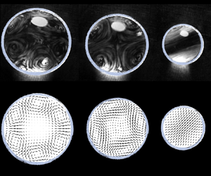
Figure 1. (a) Radius  $R$ of a Leidenfrost drop levitating on a plate heated at 350 $^{\circ }$C as a function of time $R$ decreases as $R(t)=R_0(1-t/\tau _0)$ ((2.1)), plotted as the dotted line, denoting $R_0 = 3.7\pm 0.1$ mm as the initial radius and $\tau _0 = 176.5$ s as the lifetime. (b) Drop shape for some radii $R\in [0.9 ;4.5]$ mm readable in (a) (see coloured dots). Simulated shapes (full lines), obtained by numerically integrating (2.2), are compared with experimental ones (dotted lines), obtained for side-viewed drops pinned with a needle. The scale is indicated with the capillary length $\ell _c$, that is on the order of 2.5 mm for water. Surface flows, viewed from the top, successively self-organize into (c) six counter-rotating cells (mode $m=3$), (d) four counter-rotating cells (mode $m=2$) and eventually a unique rolling cell (mode $m=1$). Drop keeps on rolling but eventually stops. The consecutive snapshots are extracted from the supplementary movie SM1, available at https://doi.org/10.1017/flo.2022.5. ( f–h) The horizontal median cut views of the most unstable mode from the numerical stability analysis for radii corresponding to (c–e). The radii for the inner flow symmetry transitions from experiments and from stability analyses are plotted is (a) as black and orange lines, respectively.
2.2 Leidenfrost drop shapes
A consequence of the time scale separation is that a given volume of liquid adopts the static shape of a non-wetting drop (Reference Roman, Gay and ClanetRoman, Gay, & Clanet, 2001). If we denote  $C(z)$ as the local curvature at a given height $z$ and $C_0$ as the curvature at the apex, the balance of hydrostatic and Laplace pressures can be written $C(z) = C_0 + z/\ell _c^2$. We introduce the curvilinear abscissa $s$, the horizontal radius at a given height $r(z)$ and the angle $\beta$ tangent to the interface. The previous equation can be recast into
 \begin{equation} \frac{\sin \beta}{r} + \frac{\mathrm{d} \beta}{\mathrm{d}s} = C_0 + \frac{z}{\ell_c^2}. \end{equation}
A numerical integration of (2) for  $\beta$ ranging from 0 to $\pi$ and $\mathcal {C}_0\ell _c$ ranging from 0.5 to 10, provides the drop shape for radii ranging from $R=0.9$ to 4.3 mm, plotted as full lines in figure 1(b). These theoretical shapes are found to match the shapes obtained for water drops kept in place by a needle (see dotted lines), except at the drop north pole, where the needle locally forms a meniscus. Increasing the drop size tends to saturate the puddle height $H$ to its maximum value $H_{max} \approx 2 \ell _c$, that is roughly 5 mm for water at 100 $\,^\circ \mathrm {C}$. Drops smaller than the capillary length $\ell _c$ are quasi-spherical while drops larger than $\ell _c$ become flattened owing to gravity. As a consequence, evaporation induces geometric changes, particularly on the drop aspect ratio $2R/H$. The presence of strong internal flows could also in principle deform the liquid interface. The Reynolds number associated with the inner flows with typical velocity $V\sim$ cm s $^{-1}$ and kinematic viscosity $\nu$ writes as $Re= R V/\nu$. For a millimetric drop, we have $Re \approx 10^3$, so that inertia overcomes viscosity. The Weber number $We$, which compares inertia with the resisting capillarity is expressed as $We=\rho _0 V^2R/\sigma _0\sim 10^{-2}$. Capillarity therefore outbalances inertia, which justifies that the drop shape does not deviate from the static ones.
2.3 Drop internal flow structure
The apparent quietness of Leidenfrost drops does not reflect what really happens inside the liquid. Side-view PIV measurements performed in a median plane of a water drop containing tracer particles have revealed strong internal flows, with velocities of a few centimetres per second. As the drop shrinks owing to evaporation, Leidenfrost flows undergo a series of successive symmetry breakings. This is further evidenced by focusing on the drop top surface. A Leidenfrost drop, kept on a concave substrate, is seeded with surface particles that have a greater affinity for the air interface. These hollow glass beads are (i) pre-dispersed in water, (ii) skimmed from the interface (where particles accumulate owing to a wetting or shape defect) and (iii) introduced into a pre-dispensed Leidenfrost drop. Despite the apparent axisymmetry of the experiment, interfacial flow structures emerge, as illustrated by the top views in figure 1(c–e) and visible in the supplementary material and movie SM1). When the drop has a radius  $R>2.5$ mm, it hosts multiple vortices, which can be described by the azimuthal wavenumber $m \geq 3$ in a cylindrical coordinate system, by denoting ( $r,\, z,\, \theta$) and using a periodic wavenumber expansion in $\theta$ as ${\rm e}^{{\rm i} m \theta },\, m\in \mathbb {N}^*$. Within the range $R=[1.8;2.5]$ mm, a mode $m=2$ clearly appears, while for smaller radius $R<1.5$ mm, the droplet rolls in an asymmetric fashion, corresponding to a mode $m=1$. Inner flows thus successively self-organize into six counter-rotating cells ( $m=3$, figure 1c); four counter-rotating cells ( $m=2$, figure 1d) and eventually a unique rolling cell ( $m=1$, figure 1e). We can notice that, at some instance in the supplementary material and movie SM1, the convective cells loose their organization and coherence. The flow structures seem to be transiently perturbed by the drop oscillation in the slightly curved well. However, the dominant modes reappear within a second as a hint of the robustness of the unstable modes. The transition from $m=2$ to $m=1$ can also be visualized by side views, using PIV techniques, as in Reference Bouillant, Mouterde, Bourrianne, Lagarde, Clanet and QuéréBouillant et al. (Reference Bouillant, Mouterde, Bourrianne, Lagarde, Clanet and Quéré2018b) (images reproduced in figures 6a and 5a) or even indirectly measured, as the drop acceleration $a$ (extracted from top views, for water drops initially at rest) suddenly increases with the mode switching to $m=1$. The experiment proposed by Reference Bouillant, Mouterde, Bourrianne, Lagarde, Clanet and QuéréBouillant et al. (Reference Bouillant, Mouterde, Bourrianne, Lagarde, Clanet and Quéré2018b) is reproduced in the supplementary material, for plate temperatures ranging from $250\,^\circ \mathrm {C}$ to $450\,^\circ \mathrm {C}$. The accelerations $a$ of approximately 80 drops as a function of their radii $R$ exhibit similar jumps from $\sim$1 mm s $^{-2}$ (in the regime where drops are flattened by gravity), up to 60 mm s $^{-2}$ as $R$ decreases to $\sim 1$ mm. This indeed corresponds to entering the self-rotation and propelling regime (Reference Bouillant, Mouterde, Bourrianne, Clanet and QuéréBouillant et al., 2018a). The onset for the transition from $m=2$ to $m=1$, referred to as $R_{2\rightarrow 1}$, is found to weakly depend on the plate temperature and to be within the interval $[1; 1.5]$ mm (see § S6 of the supplementary material).
2.4 Temperature gradient at the drop interface
To test the aforementioned thermally based instability scenario, we need to specify the thermal boundary conditions at the drop surface. The drop base is expected to be maintained at roughly the water boiling point ( $T_b = 100\,^\circ \mathrm {C}$), while its apex is cooled down by the ambient air. The temperature field in a Leidenfrost drop is measured using an infrared camera (FLIR A600 series), calibrated on the temperature range $[-40 ;+ 150]\,^\circ \mathrm {C}$, only suitable to see water, and not the brass substrate. Water being opaque to infrared wavelengths, this measurement provides the ‘skin’ temperature $T$. Figure 2 shows that, at $t = 0$, that is when $R = 3.5$ mm, $T$ linearly decreases with height $z$ (in millimetres) as $T = -3.75z + 97.0\,^\circ \mathrm {C}$, reaching a maximum $T_{max} = 97.0\,^\circ \mathrm {C}$ at the drop base ( $z = 0$). A temperature difference ${\rm \Delta} T\approx 25\,^\circ \mathrm {C}$ thus develops along the drop. At $t = 16$ s, the gradient is slightly smaller with $T = -3.53z + 97.0\,^\circ \mathrm {C}$, and it keeps decreasing as $R$ decreases. These observations are confirmed by introducing a thermocouple inside the liquid (see figure S1 in the supplementary material). For $t = 74$ s, when $R = 1.8$ mm, $T$ suddenly becomes homogeneous with $T \approx 88\,^\circ$C. As best visible in the supplementary material and movie SM1, this coincides with the moment where the flow switches to a symmetry $m=1$. At this transition, the drop starts to vibrate, which enhances mixing. For $t > 100$ s, $T$ thus becomes roughly homogeneous, with a minimum at the drop centre (along the rolling axis), and a maximum at its periphery since liquid is periodically brought close to the hot plate. In this rolling state, the liquid temperature is $T \approx 80\,^\circ$C, a value smaller than the boiling point of water, as consequences of (i) the intensifying evaporation-driven cooling; (ii) a reduction of the flattened area at the drop base from which water is heated, which scales as $R^4/l_c^2$ (Reference Mahadevan and PomeauMahadevan & Pomeau, 1999); (iii) the temperature homogenization due to the rolling-enhanced mixing. We now try to link the existence of such temperature distributions to the origin and structure of the internal flows.

Figure 2. (a) Infrared side views of an evaporating Leidenfrost water drop deposited on a slightly curved surface of brass heated at 350  $^{\circ }$C. Images, taken with a thermal camera give access to the surface temperature (calibration range from $-40\,^{\circ }$C to $+150\,^{\circ }$C to focus on the water surface). Images are extracted from supplementary material and movie SM2. (b) Surface temperature $T$ of a given water drop along its central vertical axis $z$ (white dotted line), showing the change of temperature profile as the drop radius $R$ decreases.
3. Theory
3.1 Problem formulation
Based on the experimental observations, we develop a minimal model assuming that (i) the liquid adopts at any time the static shape of a non-wetting drop; (ii) the base flow inside a drop is steady; (iii) the temperature at the bottom is fixed to the liquid boiling temperature; (iv) the interaction between the liquid and the surrounding gas is not solved completely but modelled by heat transfer correlation laws applied at the side boundary. We sketch in figure 3(a) the problem, where we represent from the side a static drop provided by (2.2). We denote by  $\Omega$ the liquid domain, and by $\partial {\varOmega}$ the boundaries, which are decomposed into $\partial {\varOmega} _F$, the upper free interface and $\partial {\varOmega} _S$, the bottom interface of the drop. We also introduce $\partial {\varOmega} _A$ the vertical centreline of the drop, the axis of symmetry. Hence, the numerical computation is done only on the half-domain $r=[0; R]$, as illustrated in figure 3(b). The bottom interface $\partial {\varOmega} _S$ is assumed to be isothermal at temperature $T_s=100\,^\circ \mathrm {C}$ (the phase change of a pure body occurs at a given constant temperature), while the temperature on the side of the drop $\partial {\varOmega} _F$ needs to be evaluated using the heat transfer balance.

Figure 3. Sketch of the problem. (a) The drop (domain  ${\varOmega}$) presents boundaries $\partial {\varOmega}$ including the upper free surface $\partial {\varOmega} _F$, the bottom interface $\partial {\varOmega} _S$ and the axis of symmetry $\partial {\varOmega} _A$. (b) Thermal conditions.
3.2 Governing equations
Under the Boussinesq approximation, the governing Navier–Stokes equation for the velocity fields  $\boldsymbol {u}=[u_r,\,u_\theta,\,u_z]^{\rm T}$ and the temperature $T$ in cylindrical coordinates $(r,\,\theta,\,z)$ defined in the domain ${\varOmega}$ of boundaries $\partial {\varOmega}$ reads
 $$\begin{align}{\frac{\partial \boldsymbol{u}}{\partial t} + \boldsymbol{u} \boldsymbol{\cdot} \boldsymbol{\nabla} \boldsymbol{u} = {-}\frac{1}{\rho_0} \boldsymbol{\nabla} p - \frac{\rho(T)}{\rho_0} \boldsymbol{g} + \nu \nabla^2 \boldsymbol{u}} \quad &{\rm in}\ {\varOmega}, \end{align}$$
 $$\begin{align}{\boldsymbol{\nabla} \boldsymbol{\cdot} \boldsymbol{u} = 0} \quad &{\rm in}\ {\varOmega}, \end{align}$$
 $$\begin{align}{\frac{\partial T}{\partial t} + \boldsymbol{u} \boldsymbol{\cdot} \boldsymbol{\nabla} T = \kappa \nabla^{2} T} \quad &{\rm in}\ {\varOmega}, \end{align}$$
where  $\boldsymbol {g}$ is the gravitational acceleration in the $z$ direction, $\nu$ the liquid kinematic viscosity and $\kappa$ its thermal diffusivity. The boundary conditions for $\partial {\varOmega} _F,\, \partial {\varOmega} _S$ and $\partial {\varOmega} _A$ are, respectively,
 $$\begin{align} {\boldsymbol{S} \boldsymbol{\cdot} \boldsymbol{n} = \boldsymbol{S}_{{gas}} \boldsymbol{\cdot} \boldsymbol{n}-\sigma(\boldsymbol{\nabla} \boldsymbol{\cdot} \boldsymbol{n}) \boldsymbol{n} + (\boldsymbol{I}-\boldsymbol{nn}) \boldsymbol{\cdot} \boldsymbol{\nabla} \sigma} \quad &{\rm on} \ \partial{\varOmega}_F, \end{align}$$
 $$\begin{align} {\boldsymbol{u\boldsymbol{\cdot} n} = 0}\quad & {\rm on } \ \partial{\varOmega}_F, \end{align}$$
 $$\begin{align} {k \boldsymbol{n} \boldsymbol{\cdot} \boldsymbol{\nabla} T = {-}h_{c} (T-T_{a}) - n' \mathcal{L}}\quad & {\rm on}\ \partial{\varOmega}_F, \end{align}$$
 $$\begin{align}{T= T_0}\quad & {\rm on} \ \partial{\varOmega}_S, \end{align}$$
with suitable boundary conditions on the flow axis of symmetry,  $\partial {\varOmega} _A$, detailed in § 3.3 for linear perturbations and reading ${u}_r={u}_\theta = 0$ for the base axisymmetric case. Here, $\boldsymbol {S}$ and $\boldsymbol {S}_{{gas}}$ are the stress tensors in the liquid and the gas, respectively, $\sigma$ is the surface tension, $\boldsymbol {n}$ the normal vector, $k$ the conductivity, $h_c$ the convective heat transfer coefficient in air, $n'$ the evaporation rate and $\mathcal {L}$ the latent heat. Equation (3.2c) expresses the heat flux balance at the interface stemming from the liquid ( $\,j_k$) transferred into air ( $j_c$) and into evaporative cooling ( $j_e$), as schematized in figure 3(b).
Both the liquid density  $\rho$ and the surface tension $\sigma$ are assumed to vary linearly with the temperature: $\rho (T) = \rho _0 (1-\beta _w(T-T_0)),\, \ \sigma = \sigma _0 - \sigma _1 (T-T_0) ,$ where $\beta _w$ is the water thermal expansion coefficient, $\beta _w= {\rho _0}^{-1} {\partial \rho }/{\partial T}$ and $\sigma _1$ the surface tension variation with the temperature, $\sigma _1= -{\partial \sigma }/{\partial T}$. We decompose now the temperature $T$ as
 \begin{equation} T = T_0 - \varTheta(r,z), \end{equation}
where  $T_0$ is the water boiling temperature taken as reference ( $T_0=100\,^\circ \mathrm {C}$) at $z=0$ and $\varTheta$ the deviation from $T_0$. The reference density $\rho _0$ and the surface tension $\sigma _0$ are defined at $T_0$. With these definitions, the density and the surface tension write
 \begin{equation} \rho(T) = \rho_0 (1-\beta_w \varTheta ) , \quad \sigma = \sigma_0 - \sigma_1 \varTheta. \end{equation}
Denoting by  $p_0$ the hydrostatic pressure, the pressure $p$ inside the liquid decomposes as $p = p_0(z) + p_1(r,\,z)$. The time, velocity and length are scaled with $H^2/\kappa,\, \kappa /H$ and $H$, respectively, where $H$ is the drop height. The temperature is scaled with the temperature difference ${\rm \Delta} T(=|\varTheta _{z=0}-\varTheta _{z=H}|)$ and the pressure is scaled with $\rho _0 \nu \kappa / H^2$, which naturally appears when plugging (3.5a–g) in (3.1a), and comparing the viscous term with the pressure term
 \begin{equation} r = H\hat{r},\quad z = H \hat{z},\quad t = \frac{H^2}{\kappa} \hat{t}, \quad \boldsymbol{u} = \frac{\kappa}{H} \hat{\boldsymbol{u}}, \quad {\varTheta} = {\rm \Delta} T \hat{\varTheta}, \quad p = \frac{\rho_0 \nu \kappa}{H^2} \hat{p}, \quad \boldsymbol{\nabla} = \frac{1}{H}\hat{\boldsymbol{\nabla}}. \end{equation}
We provide in the supplementary material Table S1 with the physical parameters relative to water, vapour, air and their interface relevant to describing our problem. We introduce the dimensionless numbers, Prandtl, Rayleigh, Marangoni, Biot and Sherwood numbers as
 \begin{equation} {Pr} = \frac{\nu }{\kappa}, \quad {Ra} = \frac{\beta_w g {\rm \Delta} T H^{3}}{\nu \kappa}, \quad Ma = \frac{\sigma_1 {\rm \Delta} T H}{\rho_0 \nu \kappa}, \quad Bi = \frac{h_{c} H}{k}, \quad Sh = \frac{h_{m} H}{D_{va}}.\end{equation}
The governing (3.1) can be now recast into
 $$\begin{align} {Pr^{{-}1} \left( \frac{\partial \hat{\boldsymbol{u}}}{\partial \hat{t}} + \hat{\boldsymbol{u}} \boldsymbol{\cdot} \hat{\boldsymbol{\nabla}} \hat{\boldsymbol{u}} \right) = {-}\hat{\boldsymbol{\nabla}} \hat{p}_1 + Ra \hat{\varTheta} \boldsymbol{e}_z + \hat{\nabla}^2 \hat{\boldsymbol{u}}} \quad &{\rm in} \ {\varOmega}, \end{align}$$
 $$\begin{align} {\hat{\boldsymbol{\nabla}} \boldsymbol{\cdot} \hat{\boldsymbol{u}} = 0}\quad & {\rm in} \ {\varOmega}, \end{align}$$
 $$\begin{align}{\frac{\partial \hat{\varTheta}}{\partial t} + \hat{\boldsymbol{u}} \boldsymbol{\cdot} \hat{\boldsymbol{\nabla}}\hat{\varTheta} = \hat{\nabla}^{2}\hat{\varTheta}}\quad & {\rm in} \ {\varOmega}, \end{align}$$
with the boundary conditions:
 $$\begin{align} {-\hat{p}_1 \boldsymbol{n} + (\hat{\boldsymbol{\nabla}} \hat{\boldsymbol{u}} + (\hat{\boldsymbol{\nabla}} \hat{\boldsymbol{u}})^T)\boldsymbol{\cdot} \boldsymbol{n} = {-} Ma ( \boldsymbol{I}- \boldsymbol{nn})\boldsymbol{\cdot} \hat{\boldsymbol{\nabla}} \hat{\varTheta}} \quad & {\rm on} \ \partial{\varOmega}_F, \end{align}$$
 $$\begin{align}{\hat{\boldsymbol{u}} \boldsymbol{\cdot} \boldsymbol{n} = 0} \quad &{\rm on} \ \partial{\varOmega}_F\ {\rm and}\ \partial{\varOmega}_S, \end{align}$$
 $$\begin{align}{\boldsymbol{n} \boldsymbol{\cdot} \hat{\boldsymbol{\nabla}} \hat{\varTheta} = {-}Bi \left( \hat{\varTheta} + \frac{T_0 -{T}_a}{{\rm \Delta} T} \right) - \frac{n'\mathcal{L}H}{k}} \quad &{\rm on} \ \partial{\varOmega}_F, \end{align}$$
 $$\begin{align}{\hat{\varTheta} = 0} \quad &{\rm on} \ \partial{\varOmega}_S, \end{align}$$
and suitable symmetry conditions on  $\partial {\varOmega} _A$ (see § 3.3 for details). The evaporation rate $n'$ is linked to the $Sh$ number, which represents the evaporative heat transfer coefficient. The heat exchanges on $\partial {\varOmega} _F$, which determine $Bi$ and $Sh$ are modelled using the Ranz–Marshall correlation (Reference Incropera, DeWitt, Bergman and LavineIncropera, DeWitt, Bergman, & Lavine, 1996; Reference Ranz and MarshallRanz & Marshall, 1952) as detailed in the supplementary material (§ S2), where the input ambient air temperature $T_a$ is also measured and provided in § S4.
3.3 Stability analysis
The steady toroidal base flow ( $\boldsymbol {u}_b,\, p_b,\,\varTheta _b$) is obtained by finding the nonlinear steady state solution of (3.1) satisfying the boundary condition (3.2) using the Newton method. The base flow is solved using the dimensional equations since some dimensionless numbers depend on ${\rm \Delta} T$, which is also an unknown of the thermal problem. (Note that the non-dimensional equation can be resolved by defining $Ra$ and $Ma$ with the known parameters, i.e. $T_s$. However, we kept the classical definitions of $Ra$ and $Ma$ which are with ${\rm \Delta} T$.) We first compute the base flows, estimate ${\rm \Delta} T$ and deduce the dimensionless numbers. This approach differs from thermoconvective studies on a flat plate or in a cylinder. In these situations, there is no radial pressure gradient and the vertical gradient is solely balanced with the density, without inducing any velocity field. The temperature difference ${\rm \Delta} T$ and thermal dimensionless parameters are control parameters. In contrast, when the radial pressure gradient is non-zero (as in the Leidenfrost configuration, owing to the boundary conditions), it induces a steady flow with non-zero velocity. Both ${\rm \Delta} T$ and the dimensionless parameters are solutions of the problem. Assuming infinitesimal perturbations on the base flow with the complex frequency ${\varOmega}$ and the azimuthal wavenumber $m$, the dimensionless flow field, pressure and temperature are decomposed using the normal mode expansion
 \begin{equation} [\hat{u}_r,\hat{u}_\theta,\hat{u}_z,\hat{p}_1,\hat{\varTheta}](r,\theta,z,t) = [{u}_r,{u}_\theta,{u}_z,{p},{\varTheta}](r,z) \exp({\rm i}m\theta - {\rm i} {\varOmega} t ) + {\rm c.c.}, \end{equation}
where c.c. indicates complex conjugate. The linearized (3.7) becomes
 $$\begin{align} {Pr^{{-}1} ( {\rm i} {\varOmega} \boldsymbol{u} + \boldsymbol{u}_b \boldsymbol{\cdot} \nabla_m + \boldsymbol{u} \boldsymbol{\cdot} \nabla_0 \boldsymbol{u}_b ) = {-}\nabla_m {p} + Ra \varTheta \boldsymbol{e}_z + \nabla^2_m \boldsymbol{u}} \quad &{\rm in} \ {\varOmega}, \end{align}$$
 $$\begin{align}{{\nabla}_m \boldsymbol{\cdot} \boldsymbol{u} = 0} \quad & {\rm in} \ {\varOmega}, \end{align}$$
 $$\begin{align}{{\rm i} {\varOmega} \varTheta + \boldsymbol{u}_b \boldsymbol{\cdot} {\nabla_m} \varTheta + \boldsymbol{u} \boldsymbol{\cdot} {\nabla_0} \varTheta_b = {\nabla}_m^{2}\varTheta} \quad & {\rm in}\ {\varOmega}, \end{align}$$
where  $\nabla _m$ represents the derivative in $\theta$ is replaced by ${\rm i}m$. The boundary conditions on $\partial {\varOmega} _F$ are
 $$\begin{align} {-{p} \boldsymbol{n} + ({\nabla}_m \boldsymbol{u} + ({\nabla}_m \boldsymbol{u})^T)\boldsymbol{\cdot} \boldsymbol{n} = {-} Ma ( \boldsymbol{I}- \boldsymbol{nn})\boldsymbol{\cdot} {\nabla}_m {\varTheta}} \quad & {\rm on}\ \partial{\varOmega}_F, \end{align}$$
 $$\begin{align}{\boldsymbol{u} \boldsymbol{\cdot} \boldsymbol{n} = 0} \quad & {\rm on} \ \partial{\varOmega}_F, \end{align}$$
 $$\begin{align}{\boldsymbol{n} \boldsymbol{\cdot} {\nabla}_m {\varTheta} = {-}Bi {\varTheta}} \quad & {\rm on}\ \partial{\varOmega}_F. \end{align}$$
Note that the perturbation temperature is now only affected by the  $Bi$ as the other heat transfer coefficients are constant and contribute only in the zero-order base flow equation. One could also linearize the last term in (3.2c) and include it in the stability analysis, but the effect on the stability results is negligible (Reference Yim, Bouillant and GallaireYim, Bouillant, & Gallaire, 2021). The condition prescribed on the drop axis of symmetry $\partial {\varOmega} _A$ (illustrated in figure 3) depends on $m$, in particular on the mode symmetry. The following conditions are thus used as in Reference Batchelor and GillBatchelor and Gill (Reference Batchelor and Gill1962):
 $$ m = 0, \quad \quad {u_r = u_\theta = \frac{\partial u_z}{\partial r} = \frac{\partial \varTheta}{\partial r} = 0}\quad\quad {\rm on} \ \partial {{\varOmega}_A},$$
 $$ m = 1, \quad\quad {u_z = \varTheta = p = \frac{\partial u_r}{\partial r} = 0 = \frac{\partial u_\theta}{\partial r} = 0} \quad \quad {\rm on} \ \partial{{\varOmega}_A},$$
 $$ m \geq 2, \quad\quad {u_r = u_\theta = u_z = \varTheta = p = 0}\quad\quad {\rm on}\ \partial{{\varOmega}_A}.$$
Finally, we prescribe on  $\partial {\varOmega} _S$ a Dirichlet condition for the temperature and a free slip condition for the velocity since the bottom surface is not in contact with the plate
 $$\begin{align} \boldsymbol{u} \boldsymbol{\cdot} \boldsymbol{n} = 0 \quad {\rm on} \ \partial{\varOmega}_S, \end{align}$$
 $$\begin{align}\varTheta = 0 {\rm on} \ \partial{\varOmega}_S. \end{align}$$
3.4 Numerical methods
All the numerical analyses are performed using FreeFEM++ software (Reference HechtHecht, 2012) for axisymmetric cylindrical coordinates  $(r,\, z)$. The velocity, pressure and temperature are discretized with Taylor–Hood P2, P1 and P2 elements, respectively. The typical number of triangles is ${\sim}10^4$. The linear equations and the eigenvalue problem are solved using UMFPACK library and the ARPACK shift–invert method, respectively. Starting with the initial radius $R=3.5$ mm, the nonlinear solution of (3.1) is solved for the given water properties. Once the solution for one radius is found, it is used as the initial guess for the smaller radius. Within five iterations, the root-mean-squared (L2) norm residual becomes smaller than $1 \times 10^{-8}$. The zero normal velocity condition on the free surface is applied using the Lagrange multiplier method (Reference BabuškaBabuška, 1973; Reference Yim, Bouillant and GallaireYim et al., 2021).
4. Numerical results
4.1 Pure buoyancy-induced flow ( $Ma=0$)

4.1.1 Base flow ($Ma=0$)

Let us first consider the case of pure buoyant flows, neglecting thermocapillary effects. The base flow is thus computed following (3.1) while setting the superficial stress on  $\partial {\varOmega} _F$ to zero. We restrict this parametric study in $R$ to the limit $R \lesssim 2$ mm, since, according to infrared measurements (figure 2), the drop surface temperature tends to homogenize, suppressing Marangoni surfaces flows. Figure 4 shows the base flow obtained in this limit of $Ma=0$, for drop radii $R=2$ mm, $R=1.3$ mm and $R=0.8$ mm, respectively. In the absence of a surface tension gradient, the base flow exhibits pure thermal convection: the flow rises along the centre axis, which is warmer since it is insulated from the drop interface, and descends along the side of the drop, where the drop is cooled. The inner velocities for purely buoyant flows ( ${\sim}1$ cm s $^{-1}$) underestimate the experimental observation ( ${\sim}5$ cm s $^{-1}$) of a similar size of drop (see figure 5(a,c) for the experimental measurements).

Figure 4. Base flows for  $Ma=0$: (a) $R=2$ mm, (b) $R=1.3$ mm and (c) $R=0.8$ mm. The temperature and velocity fields are shown in colour and with arrows. (d) Dominant growth rate ${\varOmega} _i$ of different azimuthal modes with decreasing drop radius $R$.
$R$.

Figure 5. (a,c) Velocity fields within a droplet with  $R \sim 0.9$ mm deduced from PIV measurements. (b,d) Corresponding flow fields deduced from the numerical stability analysis in the absence of Marangoni effects ( $m=1,\, Ma=0,\, Ra=6.1 \times 10^3$). Velocity arrows are plotted within the lateral (a,b) and horizontal (c,d) planes. The red dashed line in (c) indicates the area of the flattened base of the drop on which the bottom camera focuses. Colour in (b,d) indicates the perturbed temperature field (normalized with its maximum value).
4.1.2 Stability analysis ($Ma=0$)

The stability of purely thermobuoyant flows is herein considered. Figure 4(d) shows the growth rate  ${\varOmega} _i$ (imaginary part of the complex frequency ${\varOmega}$) as a function of $R$ for the modes $m=0,\,1,\,2,\,3$. A positive growth rate indicates the growth of the perturbations leading to the instability. As shown in figure 4(d), the $m=1$ mode is only unstable mode for $R>0.6$ mm. The frequency ${\varOmega} _r$ of this mode (not shown) is zero, corresponding to a steady unstable mode. The corresponding Rayleigh number $Ra$ decreases from $20\ 000$ to 10 as $R$ decreases from 2 to 0.5 mm (see figure S8b in the supplementary material), reaching the value $Ra\sim 630$ when $R\sim 0.6$ mm, for which flows become stable. Interestingly, this limit also corresponds to the radius where the droplet ability to self-rotate and propel disappears, as noticeable in the last stage of the supplementary material and movie SM1. Both the measured propelling acceleration and the droplet base asymmetry vanish below $R \lesssim 0.6$ mm until it stops (the measurement in figure 1(a) then ceases). This suggests that thermobuoyant effects become stable to non-axisymmetric disturbances and flows stabilize as the drop size reduces below a critical value. Figure 5 compares the $m=1$ unstable mode with the flow fields obtained in a Leidenfrost drop with $R \sim 0.9$ mm. The mode $m=1$ with a structure describes well the solid-like rolling motion in the experimental observation. Although the $m=1$ unstable mode with $Ma=0$ represents well the rolling motion of small drops observed in the experiments, it fails to describe the presence of higher azimuthal modes for large drops. This prompts us to look at the $Ma\neq 0$ case for larger radii.
4.2 Reduced Marangoni approximation
A major challenge for computing the base flow in a Leidenfrost drop is to be able to predict the surface tension distribution. When we take the exact surface tension temperature dependence  $\sigma _1$ provided in Table S1 (supplementary material), the Marangoni flows are largely overestimated compared with experimental observations (see figure S3 of the supplementary material). It is known, however, that Marangoni effects are very often markedly reduced (Reference Dhavaleswarapu, Migliaccio, Garimella and MurthyDhavaleswarapu, Migliaccio, Garimella, & Murthy, 2010; Reference Hu and LarsonHu & Larson, 2005a, Reference Hu and Larson2006) or even almost absent (Reference Dash, Chandramohan, Weibel and GarimellaDash et al., 2014; Reference Gelderblom, Bloemen and SnoeijerGelderblom, Bloemen, & Snoeijer, 2012; Reference Marin, Gelderblom, Lohse and SnoeijerMarin, Gelderblom, Lohse, & Snoeijer, 2011). Based on measured quantities, we first try to correct the surface tension temperature dependence $\sigma _1$. To that end, we evaluate the Rayleigh $Ra$ and Marangoni $Ma$ numbers, which compare the buoyancy and surface tension stresses in comparison with inertia, respectively, as defined in (3.6a–e). Using the parameters documented in Table S1 of the supplementary material, they are $Ra \sim 1.8 \times 10^5$ and $Ma \sim 3.6 \times 10^5$ for ${\rm \Delta} T = 25\,^\circ \mathrm {C},\, H=4$ mm, $R=3.5$ mm. Both values greatly exceed the expected critical values for the onset for Rayleigh–Bénard and Marangoni instabilities (see Table S2 in the supplementary material) – typically $Ra_c \sim O(10^3)$ and $Ma \sim O(10^2)$, for similar geometries (Reference ChandrasekharChandrasekhar, 1961). As detailed in § S7 of the supplementary material, the effective surface tension variation $\sigma _{1,eff}$ (and thus $Ma_{eff}$) is determined using numerical analysis. We select the $\sigma _{1,eff}$ that best describes the temperature difference ${\rm \Delta} T$ within the liquid (figure 2), as well as the flow velocities, typically 5 cm s $^{-1}$. The temperature profiles reported in figure 2 (left panels, $R=3.5$ mm and $R=3.0$ mm) are best represented by the curve with $\sigma _{1,eff}=4 \times 10^{-5} \sigma _1$ as shown in Figure S7 of the supplementary material for the surface temperature and figure 6 for the velocity field. The surface stress seems to be reduced by a few orders of magnitude. This has also been reported in Reference Savino, Paterna and FavaloroSavino, Paterna, and Favaloro (Reference Savino, Paterna and Favaloro2002), Reference Hu and LarsonHu and Larson (Reference Hu and Larson2002), Reference Hu and LarsonHu and Larson (Reference Hu and Larson2005b) and Reference Hu and LarsonHu and Larson (Reference Hu and Larson2006), where it is ascribed to surface contamination, or to the fact that at a large Marangoni surface stress, it is moderated by dissipation or by transport-limited properties of the fluid, reducing the achievable velocities (see figure 6 of the supplementary material). In the following stability analysis, we thus use this reduced surface tension variation by adjusting $\sigma _1$ to $\sigma _{1,eff}=4 \times 10^{-5} \sigma _1$, which is the only tuneable parameter of our study (all other physical parameters are kept to exact values of the given thermal properties, provided in Table S1).

Figure 6. (a) PIV measurements in a drop with  $R=2.5$ mm (Reference Bouillant, Mouterde, Bourrianne, Lagarde, Clanet and QuéréBouillant et al., 2018b). (b) Base flow for $Ma_{eff}=11.3$ ( $\sigma _{1,eff} = 4\times 10^{-5} \sigma _1$). The colour map and arrows give the inner temperature and velocity.
4.3 Thermocapillary flow
4.3.1 Base flow with effective $Ma$

The base flow in Leidenfrost drops is now computed as in 4.1.1, adding to thermobuoyant effects the reduced thermocapillary effects ( $\sigma _{1,eff}=4\times 10^{-5} \sigma _{1}$ and $Ma_{eff}$) shown in figure 6 compared with the experimental measurement (figure 6a). As the surface tension gradient induces Marangoni flow from low surface tension to the higher one along the surface boundary, the flow direction is opposite that of purely buoyant flow: it sinks on the centreline and rises along the surface. The typical velocity magnitude is approximately ${\sim}5$ m s $^{-1}$, a value close to what is found experimentally, which corroborates the choice of effective thermocapillary gradient done by tuning the temperature distribution in § 4.2.
4.3.2 Stability analysis with effective $Ma$

Figure 7 shows the dominant eigenvalues as a function of decreasing radius (with  $\sigma _{1,eff}=4\times 10^{-5} \sigma _{1}$). Compared with the pure buoyant flow, there exist several unstable azimuthal modes ranging from $m=1$ to 3. Figure 7(a,c,e) shows the two least stable growth rates ${\varOmega} _i$ and their corresponding frequencies ${\varOmega} _r$ are shown in figure 7(b,d, f) for azimuthal wavenumbers $m=1,\,2$ and 3. For all modes $m=1,\,2,\,3$, there exist two branches of unstable modes: one with ${\varOmega} _r=0$ (steady) and other with ${\varOmega} _r \neq 0$ (unsteady). The $m=1$ mode (figure 7a,b) is unstable both at large radius $R>2.8$ mm and small radius $R<1.3$ mm, but it shows a window of stability for intermediate values of the radius. The prevailing unstable mode for $R>2.8$ mm is unsteady, with frequency ${\varOmega} _r \,{\sim}\,10\ {\rm s}^{-1}$, while for $R<1.3$ mm, it becomes steady. Mode $m=2$ (figure 7c,d) is only unstable in the intermediate radius range $R=[2.3 ; 1.3]$ mm. At radius $R\sim 2$ mm, the unsteady branch dominates, yet with a small frequency, but the steady branch takes over at smaller $R$. Mode $m=3$ (figure 7e, f) is unstable when $R<2.8$ mm. Its steady branch dominates at large $R$ but it becomes unsteady as the radius gets closer to $R\approx 2.8$ mm. The unsteady branch of mode $m=3$ reaches a maximum growth rate around $R=2.4$ mm.

Figure 7. Growth rates and the corresponding frequencies for (a,b)  $m=1$, (c,d) $m=2$ and (e, f) $m=3$ for the two least unstable modes as a function of decreasing radius. The dominant modes for each $m$: (g) growth rate and (h) corresponding frequency.
Finally, figure 7(g,h) collects and retains only the most unstable modes  $m$ and their corresponding frequencies. We note in figure 7(g) that the axisymmetric mode $m=0$ is always stable ( ${\varOmega} _i<0$). The dependence of the dominant azimuthal mode on radius thus becomes explicit: for $R > 2.1$ mm, the mode $m=3$ is the most unstable (first steady and then oscillatory). As the radius decreases further, the $m=3$ mode becomes stable around $R=2$ mm. At $R=2.2$ mm, the mode $m=2$ starts to grow and becomes the only unstable mode in the range of radius $R=[2; 1.3]$ mm, with the maximum growth rate at $R=1.6$ mm. For $R<1.3$ mm, the steady mode $m=1$ takes over as the dominant unstable mode. This trend is very similar to the apparent mode transition in experiments, which is $m\geq 3$ for $R \gtrsim 2.8$ mm, $m=2$ for $R \approx [2.5 ; 1.8]$ mm and $m=1$ for $R \approx 1.5$ mm, as shown in figure 1. A growth rate ${\varOmega} _i \sim 1~{\rm s}^{-1}$ implies that within 2.3 s, the perturbation amplitude becomes 10 times larger than its initial value. For all modes, we verify that the growth rate is much faster than the drop evaporation rate ${\varOmega} _i \gg (1/R){\rm d}R/{\rm d}t$, underlying the quasi-steady assumption in § 2.1.
Figure 8 illustrates the eigenvectors of the most unstable mode at radii  $R=3,\,\ 1.5$ and 1 mm. The top panels display side views while the right ones show top views: $xy$ plane cut at the maximum radius $R=R_{max}$. The colours indicate temperature perturbations and the arrows are the in-plane velocity perturbations. For $R=3$ mm (figure 8a,d), the mode $m=3$ dominates. Temperature perturbations are localized along the interface and the central axis of the drop while velocity perturbations are localized where the temperature perturbations are the weakest. The top view shows three counter-rotating vortex pairs, very similar to our observations (figure 1c). For $R=1.5$ mm (figure 8b,e), the mode $m=2$ becomes the most unstable thus dominant mode. Temperature perturbations are maximum near the central axis, while velocity perturbations remain localized where temperature perturbations are weak. The top view shows four vortex cells (or two vortex pairs), in close agreement with the experiments (figure 1d). For $R=1$ mm (figure 8c, f), the displacement mode $m=1$ is the most unstable. Temperature perturbations are null on the central axis, where velocity perturbations are maximum. However, the flow structure does not match the solid-like rolling motion reported in Reference Bouillant, Mouterde, Bourrianne, Lagarde, Clanet and QuéréBouillant et al. (Reference Bouillant, Mouterde, Bourrianne, Lagarde, Clanet and Quéré2018b) and illustrated in the top of figure 1(e). We interpret this at a consequence of the temperature homogenization evidenced at small $R$ in figure 2. The temperature difference at the liquid surface indeed tends to vanish as $R$ becomes smaller than 1.8 mm. We thus expect thermocapillary effects to weaken and eventually vanish. We provide in Figure S8 (supplementary material), the (reduced) Marangoni and Rayleigh numbers with $R$, showing that both effects weaken as the drop shrinks in size, with a more abrupt decrease of thermocapillary effects than thermobuoyant effects, prompting us to use our predictions for the case $Ma=0$ when $R$ becomes sufficiently small. The observed rolling motion is thus better captured by the eigenmode for $Ma=0$ as shown in figure 5 than the one with $Ma \sim O(10)$ in figure 8(e).

Figure 8. Eigenmodes of the most unstable modes at radii (a,d)  $R=3$ mm ( $Ma_{eff}=12,\, Ra=1.5\times 10^5$), (b,e) $R=1.5$ mm ( $Ma_{eff}=9.6,\, Ra=5\times 10^4$) and (c, f) $R=1$ mm ( $Ma_{eff}=8,\, Ra=2.4\times 10^4$). Colours indicate temperature perturbations and the arrows show the in-plane velocity perturbations normalized with their maximum real values. The top view is a plane cut at the maximum radius $R=R_{max}$.
5. Discussion
We have investigated both experimentally and theoreticonumerically the Marangoni–Rayleigh–Bénard instability in a Leidenfrost drop as the cause for its complex internal dynamics. A water puddle with initial radius  $R\approx 4.0$ mm is deposited on a concave substrate brought at $T=300 \,^\circ \mathrm {C}$. Its base is warmer than its apex by typically 10 $\,^\circ \mathrm {C}$, which certainly triggers thermobuoyant and thermocapillary flows. This is confirmed experimentally: drops host very strong flows, whose symmetry is selected by the evaporation-driven confinement and change in the drop aspect ratio. Tracers reveal a self-organization from three counter-rotating cells (azimuthal modes $m=3$ for $R>2.8$ mm), to two ( $m=2$ for $R=[1.8 ; 2.8]$ mm) down a unique asymmetric rolling cell ( $m=1$ for $R\lesssim 1.5$ mm) as evaporation proceeds. In order to model this internal mode selection, we perform a numerical stability analysis of thermo-induced flows. Evaporation being three orders of magnitude slower than the convection speed inside of the liquid, the drop is assumed to be in a quasi-steady state. This is substantiated by the fact that the shape of a Leidenfrost drop, accessed with side-view imaging, matches the static shape of a non-wetting drop. The stability analysis is thus performed in quasi-static, non-deformable drops with varying radius $R$. The bottom interface is assumed to be isothermal and we model the heat transfer with the surrounding air through the Ranz–Marshall correlation laws. The base flow is computed by taking into account thermobuoyant effects (under the Boussinesq approximation), supplemented by thermocapillary effects, yet with a reduced Marangoni strength. The effective Marangoni number is tuned by matching the experimental value of the temperature difference ${\rm \Delta} T$, resulting in an effective Marangoni number of $O(10)$ (a value that predicts flow velocities close to that observed). This is much lower than the value expected for pure water, a common anomaly in thermocapillary-driven phenomena, usually ascribed to the surface contamination or for the transport-limited properties at the liquid interface. We obtain a toroidal steady base flow. A linear stability analysis reveals that the most unstable modes follow one another from $m=3 \to m=2 \to m=1$ as the radius decreases. The most unstable mode typically grows in $\lesssim O(1)$ s, which is at least ten times faster than the evaporation time scale. Figure 1(a,c–h) directly compares top view observations with the prevailing eigenmodes, obtained at the corresponding $R$. Velocity perturbation fields of the fastest growing mode, plotted in the horizontal median cut of the drop, predict flows with structures that match the experiments. The expected radii at which dominant modes switch, shown as the orange horizontal lines in figure 1(a), qualitatively agree with the experimental transition radii, shown as the black horizontal lines. The stability analysis approximately underestimates by $25\,\%$ the observed radius for the transition from $m=3 \to m=2$ and only by $15\,\%$ for the transition $m=2\to m=1$. This deviation being reasonable, we can conclude that our numerical results capture well the preferred modes selection with $R$. Premature symmetry breakings (thus slightly larger drops) indicate that the flow is more unstable than we would predict, which could be ascribed to (i) the so far neglected effect of the vapour flow; (ii) a further destabilization due to the curvature of the substrate (well geometry to keep the drop in place); (iii) liquid oscillations, which induce some variations in the equatorial radius, leading to a misreading of $R$. The case of smaller droplets ( $\lesssim 1$ mm) is more subtle. First and foremost, the vapour cushion should be considered as described in Reference Brandão and SchnitzerBrandão and Schnitzer (Reference Brandão and Schnitzer2020). Nevertheless, we made an attempt to predict the inner flow characteristics with our thermoconvective model. In this regime of size, the structure and stability of inner flows are best modelled by pure buoyancy-driven convection ( $Ma=0$), that is when thermocapillary effects are extinguished. This is corroborated by the surface temperature homogenization (see figure 2, right bottom panel at $t=74\ {\rm s}$), and the fact that Marangoni number decreases more abruptly than the Rayleigh number as $R$ decreases (see figure S8 of the supplementary material).
Our numerical model presents several limitations. The base flow calculation for a given  $R$ does not take into account the mean flow correction associated with the Reynolds stresses resulting from nonlinear perturbations and nonlinear saturation of a growing mode. Overall, it does not take into account the viscous shear from the escaping vapour underneath the drop and its coupling with the internal dynamics. This effect is expected to be weak for large drops owing to the thickening of the vapour film with $R$, yet it gains prominence as the drop gets smaller. Such a hydrodynamic scenario was found to explain symmetry breaking and spontaneous motion in capillary droplets (Reference Brandão and SchnitzerBrandão & Schnitzer, 2020). In order to arrive at a more complete picture of both the internal dynamics and the spontaneous mobility of Leidenfrost drops, it would be of interest to combine our modelling of thermoconvective effects with the (three-dimensional generalized) model recently developed for quasi-spherical drops that includes the vapour thin film (Reference Brandão and SchnitzerBrandão & Schnitzer, 2020). This would enable a discussion on the mobility associated with each mode. It would be of interest to verify the modes $m=3$ and $m=2$, which preserve a form of central symmetry, do not lead to propulsion, in contrast to the asymmetric mode $m=1$. Moreover, the drop shape is, as yet, steady, but the internal flows could be coupled to the drop envelop deformation. This extension of our model would enable the exploration of the limit of even larger drops ( $R \gtrsim 5$ mm), where star pulsations appear. Finally, it would be interesting to see how our model applies to the inverse-Leidenfrost situation (Reference Gauthier, Diddens, Proville, Lohse and van der MeerGauthier, Diddens, Proville, Lohse, & Meer, 2019), for which a rolling mode $m=1$ seems dominant for a millimetric, quasi-spherical droplet. Their configuration is, however, essentially different since temperature gradients are reversed, the drop shape remains quasi-spherical on the deformable bath and, as soon as the drop freezes, both the thermobuoyant and thermocapillary flows should extinguish.
Supplementary Material and Movies
Supplementary material and movies are available at https://doi.org/10.1017/flo.2022.5.
Declaration of Interests
The authors declare no conflict of interest.
Author Contributions
F.G. and D.Q. created the research plan, A.B. and D.Q. designed experiments, E.Y. and F.G. formulated analytical and numerical models, A.B. led model solution and performed all experiments, E.Y., A.B. and F.G. wrote the manuscript.
Data Availability Statement
Raw data are available from the corresponding author upon request.
Ethical Standards
The research meets all ethical guidelines, including adherence to the legal requirements of the study country.


 Open access