


Impact Statement
Contactless transportation using squeeze-film levitation is of rapidly growing interest in applications such as the assembly line manufacturing of touch-sensitive objects and soft-robotic locomotion over complex terrain. Achieving lateral mobility in levitation systems has typically required incorporation of multiple oscillation sources, which consume substantial energy while generating thrust forces and transport speeds that are inadequate for large-scale, practical application. The results of the present analysis demonstrate that much greater thrust can be generated by controlling systematically the inclination angle of an object levitated by repulsive or attractive pressure forces, for instance, through active control of the centre of mass of a self-levitating robot. The generality and computational efficiency of this mathematical formulation make it a versatile tool for guiding the design, optimization and closed-loop control of next-generation squeeze-film transport systems.
1. Introduction
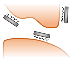
A typical squeeze-film levitation (SFL) system, as cartooned in figure 1(a), consists of two rigid objects with parallel surfaces that are separated by a slender layer of air, the ‘squeeze film’. High-frequency oscillation of either object along an axis perpendicular to the surfaces generates pulsating airflow in the film that yields a strong, steady, repulsive pressure force between the two objects. This phenomenon has been exploited to design gas-lubricated bearings (Reference SalbuSalbu, 1964; Reference Shi, Feng, Hu, Zhu and CuiShi, Feng, Hu, Zhu, & Cui, 2019) and levitation devices that exhibit large load capacities, as demonstrated, for example, by Reference ZhaoZhao (2010), who developed an ultrasonic oscillator with a small surface diameter of 5 cm that generated 115 N ( $\approx$11.7 kgf) of repulsion.

Figure 1. (a) A conventional squeeze-film levitation system can be modified to generate thrust by (b) excitation of propagating-wave surface deformations or (c) inclination of the oscillator surface.
Squeeze-film levitation systems are typically operated at a frequency that corresponds to one of the resonant bending modes of the oscillating assembly. Active feedback control of the excitation signal has been implemented to account for slight, unpredictable drifts of the natural frequency (Reference Ilssar, Bucher and FlashnerIlssar, Bucher, & Flashner, 2017). The drastic increase in the amplitude of oscillations near resonance magnifies substantially the repulsive levitation force (Reference Li, Liu and DingLi, Liu, & Ding, 2014; Reference Matsuo, Koike, Nakamura, Ueha and HashimotoMatsuo, Koike, Nakamura, Ueha, & Hashimoto, 2000). The effective flexural amplitude can be improved by reducing the stiffness of the oscillator through careful selection of material(s) (Reference Shi, An, Feng, Guo and LiuShi, An, Feng, Guo, & Liu, 2018; Reference Wang and AuWang & Au, 2013) and geometry (Reference Stolarski, Gawarkiewicz and TeschStolarski, Gawarkiewicz, & Tesch, 2015).
Under a limited range of operating conditions – namely, for surfaces with millimetric characteristic dimensions or oscillation frequencies as low as several hundred hertz – this steady force has been observed to transition from strong repulsion to weak suction of less than 1 gf (Reference Andrade, Ramos, Adamowski and MarzoAndrade, Ramos, Adamowski, & Marzo, 2020; Reference SadayukiSadayuki, 2002; Reference Takasaki, Terada, Kato, Ishino and MizunoTakasaki, Terada, Kato, Ishino, & Mizuno, 2010; Reference Yoshimoto, Shou and SomayaYoshimoto, Shou, & Somaya, 2013). Recent experiments have shown that this minor attractive load capacity is magnified a thousand fold when the stiffness of the oscillator is reduced substantially to provide pronounced flexural deformations that may be subject to non-negligible fluid–structure coupling (Reference ColasanteColasante, 2015; Reference Weston-Dawkes, Adibnazari, Hu, Everman, Gravish and TolleyWeston-Dawkes et al., 2021). A preliminary theoretical analysis (Reference Ramanarayanan and SánchezRamanarayanan & Sánchez, 2022) indicated that the range of operating conditions under which attraction occurs, as well as the magnitude of the resulting force, grows substantially with the wavenumber of oscillation, i.e. with the number of nodes in the associated standing wave, although effects of coupling remain to be understood.
Proposed applications of SFL include, primarily, assembly line manufacturing of touch-sensitive items, such as surface-mount devices for circuit boards (Reference Andrade, Ramos, Adamowski and MarzoAndrade et al., 2020) and glass substrates to be installed in liquid-crystal displays (Reference Hatanaka, Koike, Nakamura, Ueha and HashimotoHatanaka, Koike, Nakamura, Ueha, & Hashimoto, 1999), and load-carrying ‘soft’ robots that can travel over multifarious terrains (Reference Weston-Dawkes, Adibnazari, Hu, Everman, Gravish and TolleyWeston-Dawkes et al., 2021); see figure 2 for a rudimentary visualization of each. Pursuant of these applications, a number of methods have been proposed to modify the basic SFL configuration to produce also lateral forces, as reviewed in the following paragraphs.

Figure 2. Proposed applications of squeeze-film transport: (a) contactless assembly line conveyance using both repulsion (red) and attraction (blue), and (b) soft-robotic locomotion over complex terrain.
The earliest of these is the excitation of travelling-wave deformations of the oscillator, as diagrammed in figure 1(b), which generates steady, asymmetrical fluid shear on the bounding surfaces of the squeeze film. This method has been applied to develop rail-transport systems that levitate repulsively objects with masses of the order of 10–100 grams and displace them with speeds of the order of 10 cm s $^{-1}$ (Reference Ide, Friend, Nakamura and UehaIde, Friend, Nakamura, & Ueha, 2007; Reference SadayukiSadayuki, 2002; Reference YinYin, 2008). Experimenters have also designed self-levitating mobile robots with comparable masses that can produce thrust forces of the order of $10$ mN (Reference Feng, Liu and ChengFeng, Liu, & Cheng, 2015; Reference Koyama, Nakamura and UehaKoyama, Nakamura, & Ueha, 2007). The wave-generation methods employed in these experiments involve two spatially separated oscillators attached to a platform (Reference SyuhriSyuhri, 2022). Of great concern has been the purity of the travelling wave generated on the finite platform – which is limited practically by reflection at free boundaries and points of attachment, since the resulting interference may critically reduce the thrust force (Reference Feng, Liu and ChengFeng et al., 2015). Ameliorative solutions include ‘impedance matching’, where one of the oscillators acts as a passive absorber through piezoelectric energy dissipation (Reference Hariri, Bernard and RazekHariri, Bernard, & Razek, 2013; Reference SadayukiSadayuki, 2002), and ‘two-mode excitation’, where the two oscillators operate out of phase at a critical frequency that results in a favourable superposition of two consecutive resonant modes of the platform (Reference Loh and RoLoh & Ro, 2000; Reference Tomikawa, Adachi, Hirata, Suzuki and TakanoTomikawa, Adachi, Hirata, Suzuki, & Takano, 1990). Active feedback control using the latter method has been claimed to provide nearly perfect travelling waves (Reference Ghenna, Giraud, Giraud-Audine, Amberg and Lemaire-SemailGhenna, Giraud, Giraud-Audine, Amberg, & Lemaire-Semail, 2015; Reference Giraud, Giraud-Audine, Amberg and Lemaire-SemailGiraud, Giraud-Audine, Amberg, & Lemaire-Semail, 2014).
Three prominent alternative methods of transport have been proposed in recent years. The first relies on the steady shear force caused by the asymmetrical fluid streaming that occurs when a levitated object is misaligned with a finite parallel surface (Reference Yano, Aoyagi, Tamura and TakanoYano, Aoyagi, Tamura, & Takano, 2011). This so-called ‘restoring force’ is exploited by assembling an array of oscillators and controlling carefully the amplitude of each such that fluid shear conveys a levitated object along the array. Notable limitations of this method include the need for multiple oscillators, whose number and/or size must grow with the desired transport distance, and the apparent inapplicability to robotic locomotion.
Reference Chen, Gao, Pan and GuoChen, Gao, Pan, and Guo (2016) proposed a remarkable method more amenable to robotic applications – simultaneous generation of linear and rotational oscillations of a platform using a pair of independently excited piezoelectric elements, the resonant frequencies of the two oscillation modes matched using computer-aided design. In principle, if the modes are driven exactly out of phase, the oscillations should resemble a travelling wave with very large wavelength. The authors report an optimal phase shift of  $\approx 25^\circ$, which allowed a roughly $20$ g robot to travel at $2.25$ cm s $^{-1}$ and generate $30$ mN of static thrust.
The third and most recent alternative, proposed by Reference Wei, Shaham and BucherWei, Shaham, and Bucher (2018), involves inclination of the levitated object, as exemplified in figure 1(c), which would tilt the levitation force vector to provide a relatively small lateral component. This method seems particularly attractive for implementation on mobile robots, simply through active control of the on-board mass distribution. Although the robustness and stability of steady-state transport are yet to be investigated rigorously for this method, Reference Wei, Shaham and BucherWei et al. (2018) claim that it may yield substantial advantages in versatility, load capacity and controllability.
A unifying factor among the literature cited above is the focus on repulsive levitation. To the best of our knowledge, controlled transport using attraction is yet to be studied. Explored in this paper is the prospect of combining the distinct thrust-generation mechanisms of (i) travelling-wave deformations and (ii) controlled surface inclination. Results of a rigorous fluid-flow analysis indicate that both the thrust and the levitation force generated by an asymmetrical SFL system, whether the latter be repulsive or attractive, can be improved substantially through methodical adjustment of the tilting angle.
The remainder of this paper is organized as follows. Outlined in § 2 is the proposed fluid-dynamic problem that represents a generic squeeze-film system involving arbitrary flexural oscillations and a variable tilt angle. The reduced conservation equations governing fluid flow in the slender air layer are presented, followed by the introduction of appropriately rescaled dimensionless variables. An asymptotic solution is derived in § 3 and integral expressions are provided for the steady thrust force, the levitation force and the associated centre of pressure. These levitation metrics are visualized in § 4 for a variety of relevant transport configurations. The paper concludes with a discussion of possible applications of the developed formulation in system design, optimization and control.
2. Problem definition
2.1 Preliminary considerations
Consider, as a relevant canonical configuration, the planar SFL system represented in figure 3, where a plate of undeformed length  $2a$ levitates and translates above an infinitely long horizontal wall. In its undeformed state, the plate is tilted at an angle $\theta$ with respect to the wall, and its centre is separated from the wall by a time-averaged distance $h_o$. The plate undergoes time-harmonic, flexural oscillations that are described by the equation $y^* = b\,Re\{ W(x^*/a)\, \mathrm {e}^{\mathrm {i} \omega t} \}$, where $(x^*,y^*)$ specifies the depicted rotated coordinate system attached to the plate centre, $b$ and $\omega$ denote, respectively, the characteristic amplitude and angular frequency of oscillation, and $W$ is a dimensionless function that defines the waveform. For instance, the cases $W = \cos (2{\rm \pi} x^*/a)$ and $W = \exp (-2\,\mathrm {i}{\rm \pi} x^*/a)$ represent, respectively, standing waves and forward-travelling waves of wavelength $a$.
$a$.

Figure 3. A generic squeeze-film transport system: a levitated plate undergoing flexural oscillation is tilted at an angle  $\theta$ with respect to a nearby wall and propelled to the right by fluid stresses beneath.
The local pressure, temperature, density and viscosity of the oscillating gas inside the film are denoted, respectively, by  $p,T,\rho$ and $\mu$. The corresponding values of those properties in the unperturbed surroundings are denoted with the subscript ‘a’; for instance, $p_a$ denotes the ambient pressure.
For typical SFL systems (Reference Matsuo, Koike, Nakamura, Ueha and HashimotoMatsuo et al., 2000; Reference Yoshimoto, Shou and SomayaYoshimoto et al., 2013; Reference ZhaoZhao, 2010),
(i) the squeeze film is slender, $h_o \ll a$, whereby the tilt angle is small, $\theta \sim h_o/a \ll 1$;
(ii) the characteristic wavelength of the flexural oscillations is comparable to
$a$, whereby(iii) any lateral displacement
$\Delta x^*$ of points on the deforming plate surface is negligible; and(iv) the transport speed
$u_t$ is negligibly small (Reference Ide, Friend, Nakamura and UehaIde et al., 2007) compared with the characteristic speed $u_s$ of steady gaseous streaming in the film: $u_t \ll u_s \sim (b/h_o)^2 \omega a$ (Reference Ramanarayanan, Coenen and SánchezRamanarayanan, Coenen, & Sánchez, 2022).


Assumptions (i) and (ii) allow application of the slender-flow approximation (Reference Ramanarayanan, Coenen and SánchezRamanarayanan et al., 2022) to model gas flow in the film. Due to (iii) and (iv), the only non-trivial boundary condition to be imposed for the flow velocity stems from the transverse motion of the plate surface, which can now be expressed with use of the simplified equation
 \begin{equation} y = h(x,t) = h_o - x\theta + b\, Re\{ W (x/a)\, \mathrm{e}^{\mathrm{i} \omega t} \} \quad{\rm for}\ -a \le x \le a ,\end{equation}
where  $(x,y)$ denotes a coordinate system whose origin travels along the wall (see figure 3), with $x$ coincident to the wall and $y$ denoting the distance to the plate centre. The assumption of small angles $\theta \ll 1$ introduces relative errors of order $\theta ^2$ for the terms representing steady tilt and unsteady flexure.
The levitation force, defined as the vertical component of the time-averaged aerodynamic force acting on the plate (per unit length perpendicular to the plane of motion), can then be expressed as
 \begin{equation} \langle {\mathcal{F}}_L \rangle = \int_{{-}a}^a \langle p-p_a \rangle \,{\rm d}\kern0.06em x , \end{equation}
and the associated thrust force – the horizontal component – can be expressed as
 \begin{equation} \langle {\mathcal{F}}_T \rangle = \int_{{-}a}^a ( \langle p-p_a \rangle\theta - \langle \mu \partial u/\partial y \rangle |_{y = h})\, {\rm d}\kern0.06em x ,\end{equation}
both with relative errors of order  $(h_o/a)^2 \sim \theta ^2$. The angled brackets in the definitions above denote the time average of a time-dependent quantity over one period of oscillation, $\langle \star \rangle = ({\omega }/{2{\rm \pi} }) \int _{t^*}^{t^* + 2{\rm \pi} /\omega } \star \, {\rm d} t$.
In addition, the levitation moment about the plate centre and the associated centre of steady pressure can be expressed as
 \begin{equation} \langle {\mathcal{M}} \rangle = \int_{{-}a}^a \langle p-p_a \rangle x\,{\rm d}\kern0.06em x \quad{\rm and}\quad x_{csp} = \frac{\langle {\mathcal{M}} \rangle}{\langle {\mathcal{F}}_L \rangle} , \end{equation}
with the same level of accuracy. Note that, due to the simplifications employed, the quasistatic transport problem defined above also describes, in principle, systems such as those depicted in figure 2(a), where a rigid object with a flat surface (of length  $2a$) is transported over a flexurally oscillating rail.
2.2 The lubrication approximation
As shown by Reference Melikhov, Chivilikhin, Amosov and JeansonMelikhov, Chivilikhin, Amosov, and Jeanson (2016) and Reference Ramanarayanan, Coenen and SánchezRamanarayanan et al. (2022), the flow dynamics in the thin air layer of a squeeze-film system is characterized by three principal time scales – that of the driving oscillations  $t_o = \omega ^{-1}$, viscous diffusion across the film $t_v = h_o^2/(\mu _a/\rho _a)$ and acoustic pressure equilibration along the film $t_a = a/\sqrt {p_a/\rho _a}$ – which enter in the theoretical description through two non-dimensional parameters, the relevant Stokes number $\mathcal {S} = t_v/t_o$ (or, equivalently, the associated Womersley number $S^{1/2}$) and a compressibility number $\mathcal {C} = t_a/t_o$. As shown by Reference Taylor and SaffmanTaylor and Saffman (1957), the description simplifies in configurations for which $t_v \ll t_o$, whereby inertial forces are negligibly weak compared with viscous shear. In the associated lubrication limit $\mathcal {S} \ll 1$, the three time scales are found to enter through a single governing fluidic parameter
 \begin{equation} \sigma = \frac{12 \mathcal{C}^2}{\mathcal{S}} = \frac{12t_a^2}{t_ot_v} = \frac{12 \mu_a \omega a^2 }{ p_a h_o^2 } \sim 1 , \end{equation}
where the factor of  $12$ is included for consistency with the classical definition. Often referred to as the ‘squeeze number’, $\sigma$ effectively represents the combined effects of gaseous compressibility and viscous shear within the film. Solution for the case of parallel walls ( $\theta =0$) with uniform oscillation amplitude ( $W=1$) has revealed that the air near the centre of the film is entrapped due to viscous resistance, and its nonlinear response to time-harmonic compression and expansion provides the steady repulsive pressure force $\langle {\mathcal {F}}_L \rangle$ (Reference LangloisLanglois, 1962; Reference SalbuSalbu, 1964). The extent of this central region and, hence, the magnitude of the force, grows monotonically with increasing values of $\sigma$. On the other hand, as $\sigma \to 0$ and the system becomes weakly nonlinear, the force vanishes, proportional to $\sigma ^2$ (Reference Ramanarayanan, Coenen and SánchezRamanarayanan et al., 2022).
While quantifying the effects of local and convective fluid acceleration affords higher accuracy in the computation of the levitation force for a wider range of operating parameters (Reference Li, Cao, Liu and DingLi, Cao, Liu, & Ding, 2010; Reference Melikhov, Chivilikhin, Amosov and JeansonMelikhov et al., 2016; Reference Minikes and BucherMinikes & Bucher, 2006), the lubrication limit has been shown to provide excellent agreement with experimental measurements for systems with small mean distances  $h_o \ll \sqrt {\mu _a/(\rho _a \omega )}$, those that satisfy $t_v \ll t_o$, for which the strongest forces – both repulsive and attractive – are expected to occur (Reference Ramanarayanan and SánchezRamanarayanan & Sánchez, 2022; Reference SalbuSalbu, 1964; Reference ZhaoZhao, 2010). Therefore, in the following analysis, the classical compressible lubrication approximation ( $t_v/t_o \sim t_a^2/t_o^2 \ll 1$) will be employed to describe rigorously the family of transport systems schematized in figure 3. The mathematical formulation derived below may be readily extended in the future to address the general viscoacoustic limit $(t_v/t_o \sim t_a/t_o \sim 1)$ by following the methods of Reference Ramanarayanan, Coenen and SánchezRamanarayanan et al. (2022), although quantification of inertial effects would severely limit the degree of analytical development possible.
The fluid flow in asymmetrical SFL systems has been studied previously for two limiting cases that correspond to the canonical transport mechanisms drawn in figures 1(b) and 1(c). For the latter, where  $W=1$ and $\theta \neq 0$, Reference DiPrimaDiPrima (1968) outlined an asymptotic computation of the time-dependent film pressure under the assumption of a known, non-negligible transport speed. A verified numerical model, developed by Reference Wei, Shaham and BucherWei et al. (2018) using the ANSYS CFX software, provided preliminary insights into the correlation between the tilt angle and the thrust force contributed by fluid shear. For the former, where $\theta =0$ and $W=W(\xi )$, Reference Minikes, Bucher and HaberMinikes, Bucher, and Haber (2004) computed analytically the quasistatic thrust force in the case of pure travelling-wave oscillations with variable wavenumber. Reference Feng, Liu and ChengFeng et al. (2015) presented a numerical investigation of the problem for imperfect travelling waves, demonstrating the adverse effect of impurity on the thrust force. The utilized model accounted rigorously for effects of local fluid acceleration and estimated the additional drag force induced by fluid shear on the exposed plate surface.
Two notable treatments of the generic problem depicted in figure 3 must be mentioned here. Reference Minikes and BucherMinikes and Bucher (2003) presented a formulation similar to that of Reference Feng, Liu and ChengFeng et al. (2015) but computed additionally the contribution of steady overpressure to the thrust in the presence of inclination, quantifying the adverse effect of the impurity of travelling waves on the terminal transport velocity. Reference Li, Liu and ZhangLi, Liu, and Zhang (2017) addressed the stability of transport systems to disturbances in the tilt angle  $\theta$, using a model that accounts for fluid inertia but neglects the fundamental role of gaseous compressibility. They discovered a steady restoring moment that increases in magnitude with the inclination angle. However, (i) systematic modulation of thrust by controlling the inclination and (ii) achievement of transport with attractive levitation were beyond the scopes of these studies, and are explored below.
2.3 Conservation equations governing airflow in the squeeze film
Under the limit  $t_v \ll t_o$, the Navier–Stokes equations (continuity and conservation of momentum in the lateral and transverse directions) and the thermal equation of state for an ideal gas reduce, respectively, to
 \begin{equation} {\dfrac{\partial{\rho}}{\partial{t}}} + {\dfrac{\partial{(\rho u)}}{\partial{x}}} + {\dfrac{\partial{(\rho v)}}{\partial{y}}} = 0 , \quad \mu_a {\dfrac{\partial{^2u}}{\partial{y^2}}} = {\dfrac{\partial{p}}{\partial{x}}} , \quad {\dfrac{\partial{p}}{\partial{y}}} = 0 \quad{\rm and}\quad \frac{p}{p_a} = \frac{\rho}{\rho_a}, \end{equation}
with relative errors of order  $(h_o/a)^2$. In deriving the above equations, it has been assumed for simplicity that both the plate and wall surfaces are held at the ambient temperature $T_a$, whereby the conservation of energy implies that $T=T_a$ everywhere in the film. As a result, the dynamic viscosity can be considered uniform as well, $\mu (T)=\mu _a$ (Reference Chapman and CowlingChapman & Cowling, 1990). Detailed discussions of these equations, which comprise the isothermal compressible lubrication limit, are presented by Reference Taylor and SaffmanTaylor and Saffman (1957), Reference LangloisLanglois (1962) and Reference Ramanarayanan, Coenen and SánchezRamanarayanan et al. (2022).
In pursuit of a reduced dimensionless formulation of the problem, we introduce the appropriately rescaled flow variables  $\xi = x/a$, $Y = y/h_o$, $\tau = \omega t$, $U = u/(\varepsilon \omega a)$, $V = v/(\varepsilon \omega h_o)$ and $P = (p-p_a)/(\varepsilon \sigma p_a/12) = (\rho -\rho _a)/(\varepsilon \sigma \rho _a/12)$, where the quantity $\sigma$ is defined in (2.5). Note that the characteristic scales for the variations of pressure and density follow from straightforward order-of-magnitude analyses of the lateral momentum equation and the equation of state, respectively. Upon defining additionally a rescaled inclination angle $\varphi = \theta /(h_o/a)$, the plate position (2.1) can be rewritten as
 \begin{equation} \frac{h}{h_o} = H(\xi,\tau) = 1 - \varphi \xi + \varepsilon \,Re\{ W(\xi) \,\mathrm{e}^{\mathrm{i}\tau} \} , \quad{\rm where}\ \left| \varphi = \frac{\theta}{h_o/a} \right| \le 1-\varepsilon , \end{equation}
with relative errors of order  $\theta ^2$ and $\varepsilon \theta ^2$ stemming, respectively, from the terms describing tilt and flexure.
Substituting these definitions into the lateral momentum and continuity equations provides
 \begin{equation} {\dfrac{\partial{^2U}}{\partial{Y^2}}} = {\dfrac{\partial{P}}{\partial{\xi}}} \quad{\rm and}\quad \frac{\sigma}{12}{\dfrac{\partial{P}}{\partial{\tau}}} + {\dfrac{\partial{}}{\partial{\xi}}} \left[ \left( 1 + \varepsilon\frac{\sigma}{12}P \right) U \right] + {\dfrac{\partial{}}{\partial{Y}}} \left[ \left( 1 + \varepsilon\frac{\sigma}{12}P \right) V \right] = 0,\end{equation}
respectively, where  $P = P(\xi,\tau )$ due to the transverse momentum equation. The above system of equations is subject to non-slip and non-penetration conditions on the bounding walls,
 \begin{equation} U = V = 0 \quad{\rm at}\ Y = 0 \quad{\rm and}\quad U = V - \varepsilon^{{-}1} \partial H/\partial \tau = 0 \quad {\rm at}\ Y = H , \end{equation}
expressed here with errors of order  $\theta ^2$.
Upon integrating the momentum equation twice in the  $Y$ direction and applying the conditions $U(Y=0)=U(Y=H)=0$, we obtain the quasisteady Poiseuille velocity profile
 \begin{equation} U(\xi,Y,\tau) = \frac{1}{2} {\dfrac{\partial{P}}{\partial{\xi}}} Y(Y-H) , \end{equation}
involving the time-varying lateral pressure gradient  $\partial P/\partial \xi$. Substituting this result into the continuity equation, integrating across the film, applying the conditions $V(Y=0) = V(Y=H) - Re \{ W(\xi ) \,\mathrm {i} \,\mathrm {e}^{\mathrm {i}\tau } \} = 0$ and simplifying with use of the Leibniz integral rule yields the relevant Reynolds equation
 \begin{equation} \sigma{\dfrac{\partial{(PH)}}{\partial{\tau}}} - {\dfrac{\partial{}}{\partial{\xi}}} \left[ H^3 \left( 1 + \varepsilon\frac{\sigma}{12}P \right) {\dfrac{\partial{P}}{\partial{\xi}}} \right] + 12 \,Re \{ W(\xi) \,\mathrm{i} \,\mathrm{e}^{\mathrm{i}\tau} \} = 0 . \end{equation}
Two boundary conditions for  $P(\xi,\tau )$ are required to close the problem defined by (2.7), (2.10) and (2.11).
Previous studies have shown that the pressure in the squeeze film relaxes to its ambient value across small, non-slender peripheral regions that extend distances  $| \Delta \boldsymbol {x} |$ of order $h_o \ll a$ beyond the edges $\xi = \pm 1$ (Reference Ramanarayanan, Coenen and SánchezRamanarayanan et al., 2022; Reference Yoshimoto, Shou and SomayaYoshimoto et al., 2013). Due to the associated disparity of scales, the characteristic variations of pressure across these peripheries are smaller than those along the film – where $\Delta x \sim a$ – by order $h_o/a$. For arbitrary order-unity values of the relative amplitude $\varepsilon \lesssim 1$, (2.11) can therefore be readily solved using numerical methods when supplemented by the simple boundary conditions $P(\xi =\pm 1)=0$, which introduce small relative errors of $O(h_o/a \ll 1)$. Finite-difference solutions of the strongly nonlinear Reynolds equation have displayed excellent agreement with experimental results for operating conditions that fall under the lubrication limit $t_v \ll t_o$ (Reference SalbuSalbu, 1964; Reference ZhaoZhao, 2010). In the present study, numerical integration of (2.11) was performed using a straightforward central-space, forward-Euler scheme for the purpose of verifying the asymptotic solution derived below. Instructions for implementing the algorithm, as well as discussions regarding its stability, accuracy and computational efficiency, are provided by Reference MichaelMichael (1963).
3. Asymptotic solution
To allow efficient analytical reduction of the problem at hand, it will be assumed that the oscillation amplitude  $\Delta y^*=b$ is small relative to the mean thickness of the air layer, i.e. $b \ll h_o$, which allows asymptotic solution using the relative amplitude
 \begin{equation} \varepsilon = \frac{b}{h_o} \ll 1, \end{equation}
as the small perturbation parameter. Despite operating near resonance, typical SFL systems exhibit diminutive amplitudes of the order of  $b=10\ \mathrm {\mu }{\rm m}$ (Reference Andrade, Ramos, Adamowski and MarzoAndrade et al., 2020; Reference Ide, Friend, Nakamura and UehaIde et al., 2007; Reference ZhaoZhao, 2010), whereby an asymptotic solution can provide reasonable accuracy as long as the film thickness $h_o$ is relatively large (Reference Ramanarayanan and SánchezRamanarayanan & Sánchez, 2022). On the other hand, the strongly repulsive forces that are generated at close range ( $h_o \sim b$) are best quantified using a numerical solution of the Reynolds equation (Reference ZhaoZhao, 2010), as described in § 2.3, or a direct numerical simulation using the full Navier–Stokes equations (Reference Andrade, Ramos, Adamowski and MarzoAndrade et al., 2020; Reference Yoshimoto, Shou and SomayaYoshimoto et al., 2013).
Under the limit of small relative amplitudes  $\varepsilon \ll 1$, the required boundary conditions for the fluid pressure at the film edges must be developed carefully. We begin by introducing perturbation expansions for the pressure and lateral flow velocity component,
 \begin{equation} \left.\begin{array}{c} P = P_0 + \varepsilon P_1 + \cdots, \\ U = U_0 + \varepsilon U_1 + \cdots. \end{array}\right\} \end{equation}
As shall be shown in § 3, substitution of this expansion into (2.11) leads to an equation that is linear at leading order. Thus, the first term in each expansion varies harmonically with time and yields no contribution to the time-averaged levitation forces and moment, whose evaluation consequently requires the computation of first-order corrections. Due to the disparity of spatial scales between the slender film and the small non-slender regions surrounding its edges, discussed below (2.11), the leading-order pressure accepts simple relaxation conditions:  $P_0(\xi =\pm 1)=0$. However, determining the corresponding conditions for $P_1$ requires, in principle, establishing a formal asymptotic relationship between the two small parameters $\varepsilon$ and $h_o/a$, and systematically matching (Reference LagerstromLagerstrom, 1988) with the local asymptotic expansions for the pressure in the two non-slender peripheries (Reference Ramanarayanan, Coenen and SánchezRamanarayanan et al., 2022). Fortunately, for $\varepsilon \ll 1$, the reduced conservation equations that govern the peripheries under the lubrication limit are linear in the first approximation (Reference Ramanarayanan, Coenen and SánchezRamanarayanan et al., 2022). The peripheral pressure variations correspondingly exhibit a zero time average, whereby relaxation conditions can be imposed for the time-averaged first-order pressure, $\langle P_1 \rangle (\xi = \pm 1)=0$. While these conditions do not allow computation of the time dependence of $P_1(\xi,\tau )$, they are sufficient to solve for the desired steady levitation metrics (2.2)–(2.4a,b).
Substituting the expression for  $H(\xi,\tau )$ given in (2.7) along with the first two terms of the pressure expansion (3.2) into the Reynolds equation (2.11) yields
 \begin{align} &\sigma{\dfrac{\partial{}}{\partial{\tau}}} [ (P_0 + \varepsilon P_1) (1 - \varphi \xi + \varepsilon \,Re\{ W \,\mathrm{e}^{\mathrm{i}\tau} \} )] + 12 \,Re \{ W \,\mathrm{i}\,\mathrm{e}^{\mathrm{i}\tau} \} \nonumber\\ &\quad - {\dfrac{\partial{}}{\partial{\xi}}} \Big[ ( 1 - \varphi \xi + \varepsilon \,Re\{ W \,\mathrm{e}^{\mathrm{i}\tau} \} )^3 \left[ 1 + \varepsilon\frac{\sigma}{12}(P_0 + \varepsilon P_1) \right] {\dfrac{\partial{}}{\partial{\xi}}}(P_0 + \varepsilon P_1) \Big] = 0, \end{align}
which is to be solved to determine  $P(\xi,\tau )$ with small errors of $O(\varepsilon ^2)$ and $O(h_o^2/a^2 \sim \theta ^2)$.
The horizontal velocity distribution  $U(\xi,Y,\tau )$ can, in turn, be found with the same level of accuracy using the expanded form of (2.10),
 \begin{equation} U_0 + \varepsilon U_1 = \frac{1}{2} {\dfrac{\partial{}}{\partial{\xi}}}(P_0 + \varepsilon P_1) Y [ Y - ( 1 - \varphi \xi + \varepsilon\, Re\{ W \,\mathrm{e}^{\mathrm{i}\tau} \} )] .\end{equation}
3.1 Leading-order solution
Collecting terms of order unity in (3.3) leads to the linear equation
 \begin{equation} \sigma (1- \varphi \xi) {\dfrac{\partial{P_0}}{\partial{\tau}}} - {\dfrac{\partial{}}{\partial{\xi}}} \left[ (1- \varphi \xi) ^3 {\dfrac{\partial{P_0}}{\partial{\xi}}} \right] + 12 \,Re\{ W(\xi)\,\mathrm{i}\,\mathrm{e}^{\mathrm{i}\tau} \} = 0 , \end{equation}
which can be solved using the method of separation of variables. Upon substituting the ansatz
 \begin{equation} P_0 = Re \{ \varPi(\xi) \,\mathrm{e}^{\mathrm{i}\tau} \},\end{equation}
(3.5) reduces to the equidimensional ordinary differential equation
 \begin{equation} {\dfrac{{\rm d} ^2\varPi}{{\rm d} \xi^2}} - \frac{3 \varphi }{1- \varphi \xi} {\dfrac{{\rm d} \varPi}{{\rm d} \xi}} - \frac{\sigma\,\mathrm{i}}{ (1- \varphi \xi) ^2} \varPi = 12\,\mathrm{i} \frac{W(\xi)}{ (1- \varphi \xi) ^3} , \quad{\rm with}\ \varPi(\xi = {\pm} 1) = 0 . \end{equation}
Solution by the method of variation of parameters gives the reduced pressure distribution
 \begin{equation} \varPi(\xi) = \frac{ 6\,\mathrm{i} }{ \alpha \varphi (1- \varphi \xi) } \left[ L(\xi) - \frac{1 - [ (1 + \varphi )/ (1- \varphi \xi) ]^{2\alpha}}{1 - [ (1 + \varphi )/(1- \varphi ) ]^{2\alpha}} \left( \frac{1- \varphi \xi}{1- \varphi } \right)^{\alpha} L(1) \right], \end{equation}
expressed in terms of the parameter
 \begin{equation} \alpha = \sqrt{ 1 + \frac{\sigma\,\mathrm{i}}{ \varphi ^2} } ,\end{equation}
and the integral operator
 \begin{equation} L(\xi) = \frac{ \int_{{-}1}^\xi W(\tilde \xi)(1- \varphi \tilde \xi)^{\alpha-1} \,{\rm d}\tilde \xi }{ (1- \varphi \xi) ^\alpha } - (1- \varphi \xi) ^\alpha \int_{{-}1}^\xi \frac{ W(\tilde \xi) }{ (1- \varphi \tilde \xi)^{\alpha + 1} } \,{\rm d}\tilde \xi , \end{equation}
where  $\tilde \xi$ is a dummy integration variable. The reduced pressure gradient $\varPi ' = \textrm {d}\varPi /\textrm {d}\xi$ is given by
 \begin{equation} \varPi'(\xi) = \frac{6\,\mathrm{i}}{ \alpha \varphi (1- \varphi \xi) ^2 } \left[ {\tilde L}(\xi) + \frac{1 - \alpha - (1 + \alpha) [ (1 + \varphi )/ (1- \varphi \xi) ]^{2\alpha}}{1 - [ (1 + \varphi )/(1- \varphi ) ]^{2\alpha}} \left( \frac{1- \varphi \xi}{1- \varphi } \right)^{\alpha} L(1) \right] , \end{equation}
involving the additional integral operator
 \begin{equation} {\tilde L}(\xi) = (1-\alpha) (1- \varphi \xi) ^\alpha \int_{{-}1}^\xi \frac{ W(\tilde \xi) }{ (1- \varphi \tilde \xi)^{\alpha + 1} } \,{\rm d}\tilde \xi - (1 + \alpha) \frac{ \int_{{-}1}^\xi W(\tilde \xi)(1- \varphi \tilde \xi)^{\alpha-1} \,{\rm d}\tilde \xi }{ (1- \varphi \xi) ^\alpha } . \end{equation}
Finally, collecting terms of order unity in (3.4) gives the leading-order horizontal velocity distribution
 \begin{equation} U_0 = {\dfrac{\partial{P_0}}{\partial{\xi}}} \frac{ Y (Y - 1 + \varphi \xi) }{2} , \end{equation}
expressed here in terms of the gradient of the known leading-order pressure  $P_0$, given in (3.6).
Since  $P_0$ varies harmonically with time and, thus, exhibits a zero time average, i.e. $\langle P_0 \rangle = 0$, evaluation of the steady levitation metrics (2.2)–(2.4a,b) requires computation of first-order corrections.
3.2 First-order corrections
Collecting terms of order  $\varepsilon$ in (3.3) and taking the time average gives
 \begin{equation} 3 (1- \varphi \xi) ^2 \left\langle Re \{W\,\mathrm{e}^{\mathrm{i}\tau} \} {\dfrac{\partial{P_0}}{\partial{\xi}}} \right\rangle + \frac{\sigma}{12} (1- \varphi \xi) ^3 \left\langle P_0 {\dfrac{\partial{P_0}}{\partial{\xi}}} \right\rangle + (1- \varphi \xi) ^3 \left\langle {\dfrac{\partial{P_1}}{\partial{\xi}}} \right\rangle = 0 , \end{equation}
which can be integrated subject to the boundary conditions  $\langle P_1 \rangle (\xi = \pm 1) = 0$ to give
 \begin{equation} \langle P_1 \rangle (\xi) = \frac{ (1- \varphi )^2 }{ 4 \varphi } \left[ \left( \frac{1 + \varphi }{1- \varphi \xi} \right)^2 - 1 \right] \int_{{-}1}^1 G(\xi) \,{\rm d}\xi - \int_{{-}1}^\xi G(\tilde \xi) \,{\rm d}\tilde \xi ,\end{equation}
where
 \begin{equation} G(\xi) = \left\langle {\dfrac{\partial{P_0}}{\partial{\xi}}} \left( \frac{3}{1- \varphi \xi} Re\{W\,\mathrm{e}^{\mathrm{i}\tau}\} + \frac{\sigma}{12}P_0 \right) \right\rangle . \end{equation}
Upon substituting the definition of the leading-order pressure (3.6) and applying the identity
 \begin{equation} \langle Re\{ \mathcal{A}(\xi) \,\mathrm{e}^{\mathrm{i}\tau} \} \,Re\{ \mathcal{B}(\xi) \,\mathrm{e}^{\mathrm{i}\tau} \} \rangle = \frac{ Re\{ \mathcal{A}^ * \mathcal{B} \} }{2} ,\end{equation}
where  $\mathcal {A}$ and $\mathcal {B}$ are complex functions and the asterisk denotes a complex conjugate, the function $G$ can be rewritten as
 \begin{equation} G(\xi) = \frac{1}{2} Re \left\{ \varPi'^ * \left( \frac{3W}{1- \varphi \xi} + \frac{\sigma}{12}\varPi \right) \right\} ,\end{equation}
in terms of the reduced leading-order pressure  $\varPi$ and its gradient $\varPi '$, given respectively in (3.8) and (3.11). Straightforward differentiation of (3.15) yields
 \begin{equation} {\dfrac{\partial{{ \langle P_1 \rangle }}}{\partial{\xi}}} = \frac{ (1- \varphi ^2)^2 }{ 2 (1- \varphi \xi) ^3 } \int_{{-}1}^1 G(\xi) \,{\rm d}\xi - G(\xi) \end{equation}
for the time-averaged pressure gradient. Finally, collecting terms of order  $\varepsilon$ in (3.4) and taking the time average gives the steady horizontal velocity
 \begin{equation} \langle U_1 \rangle = {\dfrac{\partial{{ \langle P_1 \rangle }}}{\partial{\xi}}} \frac{Y(Y - 1 + \varphi \xi)}{2} - \frac{Y}{4} Re\{ \varPi'^ * W \} , \end{equation}
where the identity (3.17) has been employed to simplify the second term.
3.3 Non-dimensionalized levitation metrics
Once  $P_0$, $\langle P_1 \rangle$ and $\langle U_1 \rangle$ are determined, the time-averaged aerodynamic forces and moment can be expressed in the following rescaled forms, each with small asymptotic errors of $O(\varepsilon, h_o/a \sim \theta )$. Using integration by parts, one can rewrite the steady levitation force (2.2) as
 \begin{equation} \langle F_L \rangle = \frac{ 12 \langle \mathcal{F}_L \rangle }{ \varepsilon^2 \sigma p_a a} = \int_{{-}1}^1 \langle P_1 \rangle \,{\rm d}\xi = {-}\int_{{-}1}^1 \xi {\dfrac{\partial{{ \langle P_1 \rangle }}}{\partial{\xi}}} \,{\rm d}\xi , \end{equation}
and the steady moment about the plate centre (2.4a,b) as
 \begin{equation} \langle M \rangle = \frac{ 12 \langle \mathcal{M} \rangle }{ \varepsilon^2 \sigma p_a a^2} = \int_{{-}1}^1 \xi \langle P_1 \rangle \,{\rm d}\xi = {-}\frac{1}{2} \int_{{-}1}^1 \xi^2 {\dfrac{\partial{{ \langle P_1 \rangle }}}{\partial{\xi}}} \,{\rm d}\xi , \end{equation}
in terms of the steady pressure gradient. Substituting the definition of the latter, given in (3.19), one may rewrite these expressions as
 \begin{equation} \langle F_L \rangle = \int_{{-}1}^1 \xi G(\xi)\,{\rm d}\xi - \varphi \int_{{-}1}^1 G(\xi)\,{\rm d}\xi \end{equation}
and
 \begin{equation} \langle M \rangle = \bigg[ \frac{1}{2 \varphi ^2} - 1 + \frac{1}{ \varphi } \left( \frac{1- \varphi ^2}{2 \varphi } \right)^2 \ln\left( \frac{1- \varphi }{1 + \varphi } \right) \bigg] \int_{{-}1}^1 G(\xi)\,{\rm d}\xi + \frac{1}{2} \int_{{-}1}^1 \xi^2G(\xi)\,{\rm d}\xi , \end{equation}
in terms of the known function  $G$ (3.18), with the associated dimensionless centre of pressure given by
 \begin{equation} \xi_{csp} = \frac{ x_{csp} }{a} = \frac{ \langle M \rangle }{ \langle F_L \rangle } . \end{equation}
The thrust force (2.3) can be expressed in the normalized form
 \begin{equation} \langle F_T \rangle = \frac{ 12 \langle \mathcal{F}_T \rangle }{ \varepsilon^2 \sigma p_a h_o } = \langle F_T \rangle_{P} + \langle F_T \rangle_{S} , \end{equation}
as the sum of the distinct contributions of pressure and shear stress,
 \begin{equation} \langle F_T \rangle_{P} = \int_{{-}1}^1 \varphi \langle P_1 \rangle \, {\rm d}\xi = \varphi \langle F_L \rangle \quad{\rm and}\quad \left.\langle F_T \rangle_{S} = {-} \int_{{-}1}^1 {\dfrac{\partial{ \langle U_1 \rangle}}{\partial{Y}}} \right|_{Y = H} \,{\rm d}\xi , \end{equation}
respectively. Substituting the definition of  $\langle U_1 \rangle$, given in (3.20), provides
 \begin{equation} \langle F_T \rangle_{S} = {-} \frac{ \varphi }{2} \langle F_L \rangle - \frac{1}{4} Re\left\{ \int_{{-}1}^1 \varPi'^ * W \, {\rm d}\xi \right\} ,\end{equation}
where (3.21) has been used in rewriting the first term, which leads to
 \begin{equation} \langle F_T \rangle = \frac{ \varphi }{2} \langle F_L \rangle - \frac{1}{4} Re\left\{ \int_{{-}1}^1 \varPi'^ * W \, {\rm d}\xi \right\}\end{equation}
for the thrust, upon addition to the first equation in (3.27a,b). Note that, while the sign of  $\langle F_T \rangle _{P}$ is determined strictly by the direction of levitation, effects of tilt and flexure compete to determine the sign of $\langle F_T \rangle _{S}$ and, thus, also that of $\langle F_T \rangle$.
3.4 Limiting cases of interest
For SFL systems with non-parallel surfaces undergoing arbitrary flexural oscillations, the integrals required to compute the steady pressure distribution (3.15), levitation force (3.23), moment (3.24) and thrust force (3.29) must be solved numerically. Results for this general problem are presented later, obtained using vectorized global adaptive quadrature (Reference ShampineShampine, 2008) by way of the ‘integral’ function built into the MATLAB software (MathWorks, 2023).
Discussed below are three special cases that allow analytical determination of the levitation metrics, namely, systems that involve (i) parallel rigid surfaces, (ii) parallel surfaces undergoing a specific class of flexural oscillations and (iii) non-parallel rigid surfaces. Note that these three cases correspond to the simplified levitation systems represented in figures 1(a), 1(b) and 1(c), respectively.
3.4.1 Case I: $\varphi = 0$ , $W=1$


For an SFL system with parallel surfaces that undergo no elastic deformation, i.e.  $H(\tau ) = 1 + \varepsilon \cos \tau$, the reduced leading-order pressure is given by
 \begin{equation} \varPi(\xi) = \frac{12\,\mathrm{i}}{\beta^2} \left[ \frac{ \cosh(\beta\xi) }{ \cosh\beta } - 1 \right] , \quad{\rm where}\ \beta = \sqrt{\sigma} \frac{1 + \mathrm{i}}{\sqrt 2} . \end{equation}
The steady pressure distribution and levitation force are given, respectively, by
 \begin{align} \langle P_1 \rangle (\xi) = \frac{3}{\sigma} \bigg[ 5 - \left| \frac{\cosh(\beta\xi)}{\cosh\beta} \right|^2 - 4\,Re\left\{ \frac{\cosh(\beta\xi)}{\cosh\beta} \right\} \bigg] \quad{\rm and}\quad \langle F_L \rangle = \frac{30}{\sigma} \left( 1 - Re \left\{ \frac{\tanh\beta}{\beta} \right\} \right) , \end{align}
the latter of which is demonstrably identical to the solution found by Reference Minikes, Bucher and HaberMinikes et al. (2004).
Due to the lateral symmetry of  $H$ (about $\xi = 0$), the thrust and levitation moment vanish, and the centre of steady pressure is correspondingly located at the plate centre, i.e. $\langle F_T \rangle = \langle M \rangle = \xi _{csp} = 0$.
3.4.2 Case II: $\varphi = 0$ , $W(\xi ) = \sum _i C_i \xi ^{n_i} \,\mathrm {e}^{m_i\xi }$ $\{ C_i,m_i \in \mathbb {C}$ , $n_i \in \mathbb {Z}_{\ge 0} \}$


For systems with parallel surfaces undergoing flexural oscillation, where  $H(\xi,\tau ) = 1 + \varepsilon \,Re\{ W(\xi ) \,\mathrm {e}^{\mathrm {i}\tau } \}$,
 \begin{equation} \varPi(\xi) = \frac{6\,\mathrm{i}}{\beta} \left[ L(\xi) - \frac{ \sinh[ \beta(1 + \xi) ] }{ \sinh(2\beta) } L(1) \right] , \quad{\rm where}\ \beta = \sqrt{\sigma} \frac{1 + \mathrm{i}}{\sqrt 2} , \end{equation}
and the integral function  $L$ is defined as
 \begin{equation} L(\xi) = \mathrm{e}^{\beta \xi} \int_{{-}1}^\xi W(\tilde \xi)\,\mathrm{e}^{-\beta \tilde \xi} \,{\rm d}\tilde \xi - \mathrm{e}^{-\beta \xi} \int_{{-}1}^\xi W(\tilde \xi)\,\mathrm{e}^{\beta \tilde \xi} \,{\rm d}\tilde \xi . \end{equation}
The steady pressure distribution is then given by
 \begin{equation} \langle P_1 \rangle (\xi) = \frac{1 + \xi}{2} \int_{{-}1}^1 G(\xi)\, {\rm d}\xi - \int_{{-}1}^\xi G(\tilde \xi)\, {\rm d}\tilde \xi , \quad{\rm where}\ G = \frac{1}{2} Re \left\{ \varPi'^ * \left( 3W + \frac{\sigma}{12}\varPi \right) \right\} , \end{equation}
and the levitation force and moment are defined, respectively, by the simplified integrals
 \begin{equation} \langle F_L \rangle = \int_{{-}1}^1 \xi G(\xi)\, {\rm d}\xi \quad{\rm and}\quad \langle M \rangle = \frac{1}{2} \int_{{-}1}^1 \xi^2G(\xi)\, {\rm d}\xi - \frac{1}{6} \int_{{-}1}^1 G(\xi)\, {\rm d}\xi .\end{equation}
First-order corrections to the pressure give no contribution to the thrust force due to the absence of tilt ( $\varphi =0$), whereby $\langle F_T \rangle _{P}=0$ and $\langle F_T \rangle _{S} = \langle F_T \rangle = -(1/4) \,Re \{ \int _{-1}^1 \varPi '^*(\xi )W(\xi )\, \textrm {d}\xi \}$.
In their asymptotic study, Reference Minikes, Bucher and HaberMinikes et al. (2004) computed  $\langle F_T \rangle$ analytically for the case of pure travelling-wave oscillations, and utilized finite-difference methods for computing first-order pressure corrections. The generalized formulation above allows integral expression of the thrust, as well as the accompanying levitation force and moment, for arbitrary waveforms $W(\xi )$. Fully analytical computation is possible for waves of the type $W(\xi ) = \sum _i C_i \xi ^{n_i} \,\mathrm {e}^{m_i\xi }$, where each $C_i$ and $m_i$ are complex numbers and each $n_i$ is a whole number, which allow explicit integration in (3.33)–(3.35a,b). Such waves can be found, for instance, as solutions to the Euler–Bernoulli equation, which governs the dynamic bending of beams (Reference Geist and McLaughlinGeist & McLaughlin, 1994; Reference YangYang, 2005).
3.4.3 Case III: $\varphi \neq 0$ , $W=1$


For rigid-body systems with non-parallel surfaces, where  $W=1$ and $H(\xi,\tau ) = 1 - \varphi \xi + \varepsilon \cos \tau$, the reduced leading-order pressure assumes the form
 \begin{equation} \varPi(\xi) = \frac{12\,\mathrm{i}}{ \varphi ^2\alpha^2} \frac{1}{1- \varphi \xi} \left[ \frac{ (1- \varphi ^2)^\alpha (1- \varphi \xi) ^{-\alpha} + (1- \varphi \xi) ^{\alpha} }{ (1 + \varphi )^\alpha + (1- \varphi )^\alpha } - 1 \right] , \end{equation}
with  $\alpha$ defined in (3.9). Analytical expressions for the steady levitation metrics can be found through tedious but straightforward algebra. Most notably, the contribution of shear stress to the thrust force is opposite in direction and half in magnitude to that of film pressure. This can be shown simply by substituting $W=1$ into (3.28), which gives $\langle F_T \rangle _{S} = - \varphi \langle F_L \rangle /2 = -\langle F_T \rangle _{P}/2$.
Of practical interest is the behaviour of the solution when the film thickness is severely reduced and, thus, the greatest repulsive levitation forces are expected to occur (Reference ZhaoZhao, 2010). In the associated limit  $\sigma \to \infty$, the steady overpressure distribution simplifies to $\langle P_1 \rangle (\xi ) = 15 / [ \sigma (1- \varphi \xi ) ^2 ]$, not accounting for the rapid relaxation of $\langle P_1 \rangle$ to zero at the edges of the film $\xi =\pm 1$ (Reference DiPrimaDiPrima, 1968). The corresponding levitation force and moment assume the simplified forms
 \begin{equation} \lim_{\sigma\to\infty} \langle F_L \rangle = \frac{30}{\sigma(1- \varphi ^2)} \quad{\rm and}\quad \lim_{\sigma\to\infty} \langle M \rangle = \frac{15}{\sigma \varphi ^2} \left[ \ln\left( \frac{1- \varphi }{1 + \varphi } \right) + \frac{2 \varphi }{1- \varphi ^2} \right] .\end{equation}
4. Discussion of results
4.1 Time-averaged squeeze-film pressure
Exemplified in figure 4 are normalized distributions of the time-averaged first-order pressure  $\langle P_1 \rangle (\xi )$ for the three limiting cases discussed above and represented in figure 1(a–c): (a) rigid bodies with parallel surfaces, (b) parallel surfaces with travelling-wave oscillations $W=\exp (-2\,\mathrm {i}{\rm \pi} \xi )$ and (c) rigid bodies with a surface tilt ratio of $\varphi = \theta /(h_o/a) = 0.2$. For all three cases displayed, $\langle P_1 \rangle (\xi )$ depends strongly on the squeeze number $\sigma = 12 \mu _a \omega a^2 / (p_a h_o^2)$. In particular, when $\sigma \gg 1$ and effects of gaseous compressibility are correspondingly augmented, as discussed below (2.5), the overpressure varies gradually within the film and relaxes sharply near its edges, in agreement with prior results (Reference DiPrimaDiPrima, 1968; Reference Ramanarayanan, Coenen and SánchezRamanarayanan et al., 2022; Reference SalbuSalbu, 1964).

Figure 4. Sample profiles of the normalized time-averaged film pressure for SFL systems with (a) zero flexure and zero tilt, (b) pure travelling-wave flexure and (c) non-zero tilt. Asymptotic results (continuous and dotted curves) are verified with numerical solutions of (2.11) for  $\varepsilon =0.01$ (dots and circles). Results are shown for (a) $W=1, \varphi =0$, (b) $W=\exp (-2\textrm {i}{\rm \pi} \xi ), \varphi =0$ and (c) $W=1, \varphi =0.2$.
For a flexible plate undergoing travelling-wave deformations, the steady overpressure distribution becomes largely negative for critically small values of  $\sigma$, in agreement with prior results that demonstrate a strong correlation between flexural oscillations and the emergence of suction forces in SFL systems (Reference Ramanarayanan and SánchezRamanarayanan & Sánchez, 2022). It is of interest to understand the behaviours of such systems because of their potential to provide controlled transport with attractive levitation, a phenomenon that is yet to be demonstrated with rigorous experimentation.
For a rigid plate with a positive inclination angle, the steady pressure distribution is skewed such that  $\langle P_1 \rangle$ assumes larger values near the lowered leading edge $\xi = 1$. Correspondingly, while the steady film pressure yields a positive contribution $\varphi \langle F_L \rangle$ to the thrust, the steady shear force caused by first-order streaming acts in the opposite direction, reducing $\langle F_T \rangle$ by a factor of two, as noted below (3.36).
4.2 Visualization of levitation metrics
In pursuit of a practical understanding of the generic SFL transport system outlined in figure 3, it is of interest to delineate clearly – i.e. in a manner amenable to physical interpretation – the parametric dependences of the steady levitation metrics on the tilt ratio  $\varphi =\theta /(h_o/a)$, flexural waveform $W(\xi )$ and squeeze number $\sigma =12\mu _a\omega a^2/(p_a h_o^2)$.
Although these three governing parameters are considered to be ‘independent’ under the present formulation, variations in  $\sigma$ can, in practice, affect $W$. In particular, since SFL oscillators typically operate near resonance (Reference Ilssar, Bucher and FlashnerIlssar et al., 2017), altering their excitation frequency $\omega$ or length $2a$ may disturb substantially the amplitude $b$ and wavelength of their flexural deformations. Therefore, it seems most appropriate to interpret the variation with $\sigma$ of the levitation forces and moment as a variation with the levitation height $h_o$. The latter is typically a ‘dependent’ variable that responds freely to changes in the load $\langle {\mathcal {F}}_L \rangle$, for instance, the change in apparent weight of a mobile robot as it travels along a curved path as in figure 2(b) (Reference Weston-Dawkes, Adibnazari, Hu, Everman, Gravish and TolleyWeston-Dawkes et al., 2021). (Note that, for oscillators with sufficiently low mass or flexural rigidity, $b$ and $W$ may be affected significantly by variations in $h_o$ and the tilt angle $\theta$ (Reference Ilssar and BucherIlssar & Bucher, 2017; Reference Weston-Dawkes, Adibnazari, Hu, Everman, Gravish and TolleyWeston-Dawkes et al., 2021); such coupled interactions are not considered below.)
Correspondingly, in representing the present asymptotic results, it is convenient to renormalize the steady levitation and thrust forces according to
 \begin{equation} L = \left( \frac{\sigma}{12} \right)^2 \langle F_L \rangle = \frac{ \langle {\mathcal{F}}_L \rangle }{ b^2 p_a^2/(\mu_a \omega a) } \quad{\rm and}\quad T = \left( \frac{\sigma}{12} \right)^{3/2} \langle F_T \rangle = \frac{ \langle {\mathcal{F}}_T \rangle }{ b^2 p_a^{3/2} / (a \sqrt{\mu_a \omega})},\end{equation}
where multiplication by an appropriate power of  $\sigma$ has eliminated $h_o$. Upon introducing also a normalized height
 \begin{equation} {\bar h}_o = \frac{1}{\sqrt \sigma} = \frac{h_o}{ 2a \sqrt{3\mu_a \omega/p_a}} , \end{equation}
the dimensionless functions  $L( {\bar h}_o )$ and $T( {\bar h}_o )$ can be interpreted to represent the variations of the levitation and thrust forces with the mean levitation height, for a given tilt ratio and flexural mode.
Displayed in figures 5 and 6 are the variations with  ${\bar h}_o$ of $L$,
$L$,  $T$ and the centre of steady pressure $\xi _{csp}$ for the canonical transport systems pictured in figures 1(b) and 1(c), respectively. It may be readily noted from both figures that the limiting behaviours of $L$ for small and large values of ${\bar h}_o = 1/\sqrt {\sigma }$ are consistent with prior knowledge concerning the role of gaseous compressibility in SFL systems, the latter elucidated below (2.5). The behaviour of the solution for intermediate levitation heights ${\bar h}_o \sim 1$, however, differs substantially between the two cases and will be discussed below.

Figure 5. Variation with the normalized levitation height  ${\bar h}_o$ (4.2) of the dimensionless (a) levitation and (b) thrust forces (4.1a,b) and (c) the centre of steady pressure (3.25), for a travelling-wave-driven system with varying wavenumber $K$. Curves labelled ‘impure’ are computed for a wave purity of $\mathcal {P} = 0.5$ (4.3).

Figure 6. Variation with the normalized levitation height  ${\bar h}_o$ of the dimensionless (a) levitation and (b) thrust forces and (c) the centre of steady pressure $\xi _{csp}$ for a rigid-body SFL system, for various values of the tilt ratio $\varphi$ (2.7). Limiting values of $\xi _{csp}$ for ${\bar h}_o \to 0$ (broken lines) are found using (3.25) and (3.37a,b).
4.3 Transport by travelling-wave oscillations
The solid curves in figure 5 represent the levitation metrics for systems with parallel surfaces ( $\varphi =0$) driven by pure travelling waves $W=\mathrm {e}^{-\mathrm {i} K\xi }$, where $K$ is the relevant dimensionless wavenumber that has been normalized with the inverse of the semi-length $a$.
$a$.
As seen respectively in panels (a) and (b), the levitation force is significantly reduced by flexure within the displayed range of heights  ${\bar h}_o$, and the thrust force exhibits a finite maximum at a critical height that varies with $K$. Investigation of the limit ${\bar h}_o \to 0$ (or, equivalently, $\sigma \to \infty$) reveals that curves of $L$ for all values of $K$ eventually converge in the case of pure travelling waves, in agreement with the findings of Reference Minikes, Bucher and HaberMinikes et al. (2004), who noted that optimization of these systems for repulsive operation warrants compromising between a levitation force that increases for decreasing values of ${\bar h}_o$ and a thrust force that varies non-monotonically.
Furthermore, as seen in figure 5(c), the centre of pressure varies strongly with  ${\bar h}_o$, indicative of a non-negligible sensitivity to levitation height that must be taken into account when designing and controlling a mobile robot or a rail-transport system. Interestingly, $\xi _{csp}$ exhibits a singularity at a critical height that corresponds to a state of zero levitation. Beyond this critical height, $L$ assumes negative values, corresponding to attractive levitation (see the associated distribution of steady film pressure exemplified in figure 4c). Both the attractive load capacity and the maximum thrust rise with increasing values of the wavenumber $K$.
$K$.
As noted previously, generation of pure travelling-wave deformations of a finite body is hindered by the reflection of propagating waves at open boundaries and points of actuation. The resulting impure travelling waves can be modelled approximately with use of the modified waveform
 \begin{equation} W = \cos(K\xi) - \mathrm{i} \mathcal{P} \sin(K\xi) , \quad{\rm with}\ 0 \le \mathcal{P} \le 1 , \end{equation}
where  $\mathcal {P}$ constitutes a coefficient of purity. Namely, when $\mathcal {P} = 1$, $W$ parametrizes the classical travelling wave $\mathrm {e}^{-\mathrm {i} K\xi }$, and when $\mathcal {P} = 0$, a perfect standing wave of equal wavenumber and amplitude (Reference Feng, Liu and ChengFeng et al., 2015; Reference Minikes and BucherMinikes & Bucher, 2003). Note that the inverse of $\mathcal {P}$ is often referred to in literature as the ‘standing-wave ratio’. As exemplified by the dotted curves in figures 5(a) and 5(b), introduction of impurity in a travelling-wave-driven SFL system seems to improve the attractive load capacity, but reduces drastically the maximum thrust force that can be produced.
4.4 Effects of surface inclination
Represented in figure 6 are the levitation metrics for a rigid-body system ( $W=1$) with various tilt ratios $\varphi = \theta /(h_o/a)$. Recall that $\varphi$ is a dimensionless representation of the amount of tilt where, for any given levitation height $h_o$, $\varphi =0$ denotes parallel surfaces and $\varphi =\pm (1-\varepsilon )$ denotes maximum tilt in either direction – i.e. the leading or trailing edge of the plate comes into contact with the wall during each downward stroke of the oscillation cycle.
It is clear from figures 6(a) and 6(b) that tilting the plate about its centre substantially increases the levitation and thrust forces at any given operating height  ${\bar h}_o$. Both appear to increase unboundedly as ${\bar h}_o \to 0$, assuming substantially greater values than those produced by flexure-driven systems, for the range of ${\bar h}_o$ displayed. Indeed, in the associated limit of large $\sigma$ (3.37a,b), $L$ becomes proportional to the inverse square of the levitation height ${\bar h}_o ^{-2}$, well in agreement with prior research (Reference Taylor and SaffmanTaylor & Saffman, 1957), and $T \propto {\bar h}_o ^{-1}$. Of course, both are physically limited since $h_o$ cannot decrease below the amplitude $b$ (Reference ZhaoZhao, 2010). Finally, figure 6(c) demonstrates that the centre of steady pressure moves toward the leading edge with increasing tilt and varies rather weakly with ${\bar h}_o$. The associated steady moment acts to reduce the angle of inclination, in agreement with the findings of Reference Li, Liu and ZhangLi et al. (2017).
One may anticipate that these effects of surface inclination apply also to systems with non-uniform oscillations, for which d $W/$d
$W/$d $\xi \neq 0$. Firstly, the sensitivity of $\xi _{csp}$ to perturbations in levitation height can be expected to increase with the onset of flexure near resonance, accompanying a possible transition to attractive levitation forces (Reference Ramanarayanan and SánchezRamanarayanan & Sánchez, 2022). For systems with lateral symmetry, where $W(-\xi ) = W(\xi )$ for $0 < \xi \le 1$, inclination in either direction is expected to (i) provide significant thrust and (ii) increase substantially the existing repulsive levitation force. Systems undergoing asymmetrical oscillations require further investigation.
Visualized using solid curves in figure 7, for example, are the levitation metrics of a system driven by pure travelling waves, for various values of the tilt ratio  $\varphi$. As seen in panel (a), positive and negative inclination increase substantially the repulsive and attractive load capacities, respectively. The aptly rescaled steady pressure distributions that correspond to the state of maximal attraction are compared in panel (c) for $\varphi =\theta /(h_o/a)=0$ and $-0.5$. Panel (b) reveals that inclination in either direction increases also the thrust force $T$ for a wide range of levitation heights ${\bar h}_o$, due to the combined contributions of fluid shear (stemming from wave propagation) and pressure (from surface tilt). The dotted curves in panels (a–c) indicate, however, that the degree of purity of the travelling wave significantly impacts the extent to which these benefits may be realized practically. Panel (d), where only pure travelling waves are considered for purposes of visual clarity, confirms the high variability of the centre of steady pressure that accompanies the transition from repulsion to attraction for flexural systems.

Figure 7. Variation with the normalized levitation height  ${\bar h}_o$ (4.2) of the rescaled (a) levitation force (4.1a,b), (b) thrust and (d) centre of steady pressure (3.25), for a flexural system with wavenumber $K=2{\rm \pi}$. Curves are shown for various tilt ratios $\varphi$ (2.7) and wave purities $\mathcal {P}$ (4.3); curves labelled ‘impure’ are computed for $\mathcal {P} = 0.5$. Plotted in (c), and verified numerically for $\varepsilon =0.01$ (dots and circles), are profiles of steady pressure for states where the system produces maximal attraction, marked with triangles in (a) and (b).
4.5 Optimization of travelling-wave-driven systems with variable inclination
Based on the preliminary results above, it appears that incorporating the mechanism of controlled inclination may improve the effectiveness of transport systems driven by impure travelling-wave oscillations for purposes of both repulsive and attractive SFL. To quantify precisely the extent of improvement that may be gained, we conclude this paper with a rigorous investigation of the associated generalized problem.
As discussed in § 1, the purity  $\mathcal {P}$ of a travelling wave is limited by the effectiveness of the wave-generation method, and the wavenumber $K$ is typically determined by the chosen natural frequency and geometric properties of the oscillator. Active feedback control is often employed to ensure that the resulting waveform $W$ remains constant during operation. In contrast, the levitation height ${\bar h}_o$ and tilt ratio $\varphi$ are free to respond to (i) perturbation by external forces and/or (ii) active adjustments to the mass or centre of mass of the levitated object. In pursuit of quantifying the maximal capabilities of travelling-wave-driven SFL systems that feature controllable inclination, we therefore explore the parametric domain spanned by ${\bar h}_o$ and $\varphi$, for a fixed wavenumber $K=2{\rm \pi}$ and select values of $\mathcal {P}$.
Two important distinctions must be drawn at this point between the mobile robot depicted in figure 2(b) and the rail-transport system schematized in figure 2(a). In the case of the former, the oscillator is attached to the levitated object, such that the waveform  $W$ is invariant as the object travels. In contrast, for rail-transport systems, the wave is subject to a phase shift that evolves as the object translates, whereby stationary components in the wave can cause fluctuations in the levitation forces and moment. The resulting operational instabilities may be especially pronounced for travelling waves with lower purity $\mathcal {P}$ and relative wavenumber $K$ (Reference Hashimoto, Koike and UehaHashimoto, Koike, & Ueha, 1996; Reference Liang, Ling and ZhangLiang, Ling, & Zhang, 2010; Reference SadayukiSadayuki, 2002). Secondly, the mass distribution of a self-levitating mobile robot may be adjusted actively to control the inclination $\varphi$, but that of a levitated object in a rail-transport system is typically fixed. Both of these distinctions must be considered carefully when interpreting and applying practically the following results.
The performance objective(s) for an SFL system will vary with the desired transportation path, for instance, translation (i) above a horizontal surface, (ii) below a horizontal surface, (iii) upward or downward along a vertical surface or otherwise (see figure 2 for clarificatory illustrations).
For transport above a horizontal surface, possible objectives include maximizing the repulsive levitation force  $L$ and/or the thrust $T$. Based on the results outlined in figures 5–7, $L$ and $T$ may be maximized by increasing the positive tilt angle and the wave purity, respectively, as much as physically possible.
For transport below a horizontal surface, it may be of interest to maximize the attractive levitation force  $(-L)$ and/or the thrust $T$. As seen, for example, in figures 5 and 7, $L$ may exhibit a negative global minimum for a critical levitation height ${\bar h}_o = {\bar h}_o ^*$. Plotted in figure 8 are the non-monotonic variations with $\varphi$ of this maximal attractive force $L( {\bar h}_o ^*)$ and the corresponding thrust $T( {\bar h}_o ^*)$ for various values of $\mathcal {P}$, demonstrating that there is a critical range of tilt ratios for which the performance of such a system is maximized. For instance, when $\mathcal {P}=0.5$, an inclination of $-0.4 \lessapprox \varphi \lessapprox -0.25$ is most desirable. Note that the benefits of controlled inclination are greater for purer travelling waves. Of practical concern is the fact that systems operating at this critical height are unstable to positive perturbations in ${\bar h}_o$ – that is, $\partial L/\partial {\bar h}_o > 0$ for ${\bar h}_o > {\bar h}_o ^*$. For this reason, operating below the maximum capacity, at a height ${\bar h}_o < {\bar h}_o ^*$, is recommended for avoiding catastrophic failure during attractive levitation.

Figure 8. Variation with the tilt ratio  $\varphi$ of (a) the normalized critical levitation height at which a travelling-wave-driven system with wavenumber $K=2{\rm \pi}$ generates maximal attraction, and the corresponding values of (b) the levitation force $L$ and (c) the thrust $T$, for three values of the wave purity $\mathcal {P}$ (4.3). For the case $\mathcal {P}=0.5$, $L$ and $T$ are verified with numerical solutions computed for $\varepsilon =0.01$ (circles).
Finally, for vertical transport along an upright surface, the thrust force must be maximized while the levitation force  $L$ must be identically zero. As seen, for example, in figures 5 and 7, the function $L( {\bar h}_o )$ may vanish at a critical height ${\bar h}_o '$, corresponding to a transition from repulsive to attractive levitation. A system that operates at this height is necessarily stable to positive and negative perturbations in ${\bar h}_o$ – i.e. $\partial L/\partial {\bar h}_o < 0$ for ${\bar h}_o = {\bar h}_o '$. Plotted in figure 9 is the variation with the tilt ratio $\varphi$ of the corresponding thrust force $T( {\bar h}_o ')$ for various values of the wave purity $\mathcal {P}$. Once again, there appears to be a desirable range of tilt ratios for which performance is maximized, with greater benefits obtained for purer oscillations.

Figure 9. Variation with the tilt ratio  $\varphi$ of (a) the normalized critical levitation height at which a travelling-wave-driven system with wavenumber $K=2{\rm \pi}$ generates zero levitation force and (b) the corresponding value of the thrust force $T$, for three values of the wave purity $\mathcal {P}$ (4.3). For the case $\mathcal {P}=0.5$, asymptotic results for $T$ are verified with numerical solutions computed for $\varepsilon =0.01$ (circles).
These analyses may be readily extended to address more complex design problems, those that may require inclined transport paths and involve performance criteria that concern simultaneously the levitation force  $\langle {\mathcal {F}}_L \rangle$, thrust $\langle {\mathcal {F}}_T \rangle$ and stability to perturbations in the tilt angle $\theta$.
5. Conclusions
Developed in this paper is a theoretical description of the planar, viscous, compressible airflow in contactless transport systems that operate using SFL. The reduced asymptotic formulation, which accounts for non-uniform structural oscillations of non-parallel surfaces, provides fundamental insights into the fluidic mechanisms that underlie thrust generation in squeeze-film systems, and enables rapid computation of their performance characteristics using integral expressions.
Particular attention is dedicated to studying the influence of surface inclination on transport systems that are driven by impure travelling waves (see figures 2 and 3). Results demonstrate that controlled modulation of the tilting angle can improve substantially the maximum achievable thrust as well as the load capacity for systems that operate using both repulsive and attractive levitation. In the case of the latter, the amount of improvement that can be gained depends strongly on the purity of the travelling wave, or more generally, presumably on the degree of lateral asymmetry in the flexural oscillations.
Sample computations are provided to display the potential of the present formulation in serving as an efficient tool to supplement the design, optimization and active control of mobile robots. The accuracy and versatility of this theoretical model must be improved in the future by modelling appropriately the effects of non-negligible transport speeds (Reference DiPrimaDiPrima, 1968), free vibrations of the levitated object (Reference Ilssar and BucherIlssar & Bucher, 2017; Reference YoshimotoYoshimoto, 1997), fluid–structure coupling by which the flexural waveform of the oscillator may alter in response to changes in levitation height and tilt angle (Reference Weston-Dawkes, Adibnazari, Hu, Everman, Gravish and TolleyWeston-Dawkes et al., 2021), fluid inertia and the accompanying relaxation of steady pressure beyond the boundaries of the squeeze film (Reference Ramanarayanan, Coenen and SánchezRamanarayanan et al., 2022) and surface roughness, which can substantially reduce the levitation force and transport speed (Reference Chen, Gao, Pan and GuoChen et al., 2016; Reference Weston-Dawkes, Adibnazari, Hu, Everman, Gravish and TolleyWeston-Dawkes et al., 2021).
Acknowlegements
We gratefully acknowledge insightful conversations with Dr Tolley and Mr Chengze-Jia regarding the practical applicability of transport using attractive SFL.
Declaration of interests
The authors declare no conflict of interest.


 Open access