


1. Introduction
Mathematical modeling of pedestrian dynamics has a practical benefit in civil engineering [Reference Khelfa, Korbmacher, Schadschneider and Tordeux23, Reference Schadschneider, Chraibi, Seyfried, Tordeux and Zhang26, Reference Schadschneider, Klüpfel, Kretz, Rogsch and Seyfried27] for example in the design of complex architectures, e.g., stadiums, city centers, and shopping malls, or for the management of large public events like festivals, concerts, pilgrimages, or manifestations [Reference Chraibi, Tordeux, Schadschneider and Seyfried10]. Capturing both, the individual and collective behaviors in pedestrian dynamics, is rather complex [Reference Bellomo, Gibelli, Quaini and Reali2, Reference Castellano, Fortunato and Loreto7]. Many different approaches have been proposed in the literature: for example, models based on magnetic forces proposed by S. Okazaki and S. Matsushita in which pedestrians are modeled as magnetic charges in a magnetic field [Reference Teknomo, Takeyama and Inamura33]; the gas-kinetic model which treats pedestrians as molecules in liquefied gas [Reference Hoogendoorn and Bovy22]; cellular automata [Reference Burger, Hittmeir, Ranetbauer and Wolfram4, Reference Burstedde, Klauck, Schadschneider and Zittartz5, Reference D’Orsogna, Chuang, Bertozzi and Chayes.13]; models incorporating anticipative, rational behavior [Reference Bailo, Carrillo and Degond1, Reference Christiani, Priuli and Tosin11, Reference Dijkstra, Jessurun and Timmermans12] and (smooth) sidestepping [Reference Festa, Tosin and Wolfram15, Reference Totzeck34]. Another group of pedestrian models has emerged from the pioneering work on social forces [Reference Helbing and Molnar20] and can be classified as force-based [Reference Chraibi, Kemloh and Seyfried9, Reference Totzeck34] and the overview given in [Reference Chen, Treiber, Kanagaraj and Li8].
Most of these models share the property of reproducing collective features such as lane formation in counter-flow scenarios and traveling waves in crossing flows. Moreover, they can be used to study evacuation scenarios. On the other hand, they strongly differ in their description. Indeed, some models, for example, the class of forces-based models have a sound mathematical description and allow for a statement in terms of a closed system of ordinary or partial differential equations. Others have a rather algorithmic structure because they require the solution of optimization problems to estimate for example the time-to-collision in every iteration. For the latter, a rigorous mathematical study of well-posedness is difficult.
Naturally, the modeling process is followed by an optimization or calibration procedure. For pedestrian dynamics, the optimization of buildings, evacuation routes, and traffic safety or the minimization of the occurrence of high densities are of special interest [Reference Seitz28, Reference Zhou, Dong, Ioannou, Zhao and Wang37]. Moreover, the collection of data from real-world experiments grew the interest in parameter fitting for the different pedestrian models [Reference Bode and Ronchi3, Reference Gomes, Stuart and Wolfram17, Reference Göttlich and Totzeck18].
This work is in a similar spirit. First, we extend the anisotropic model proposed in [Reference Totzeck34] by incorporating a body size for the interacting agents. This induces another dimension of volume exclusion in the model and makes the model more realistic. However, it is simple enough to derive the gradient used for the optimization explicitly. We emphasize that this is exceptional, as many other particle models for pedestrian dynamics include terms like the Heaviside function in the social force model or an optimization problem in their dynamics that prohibit the straight forward computation of adjoints and gradients. We study the influence of the body size on the formation of lanes and traveling waves as well as the fundamental diagram of the dynamics numerically and provide a rigorous study of the well-posedness of the interaction dynamics with and without body size employing standard ODE theory. The second part of the article is concerned with the rigorous derivation of a gradient-based parameter calibration algorithm. We begin with the derivation of the first-order optimality system and propose a mini-batch gradient-descent algorithm for the calibration problem.
In more detail, the article is organized as follows: the anisotropic model for pedestrian dynamics is extended by including the agents’ body size in Section 2. Moreover, we study the influence of body size on collective behavior and the fundamental diagram in there. Section 3 is devoted to the parameter calibration problem. We begin with the statement of the problem, investigate its well-posedness, and derive the corresponding first-order optimality conditions. Finally, the iterative gradient descent algorithm based on mini-batches for the parameter calibration is proposed in Section 4, where we show results obtained with this algorithm. We conclude with a summary of the results and an outlook on future projects.
2. Microscopic model with body size
We include the body size in the anisotropic model proposed in [Reference Totzeck34] as follows: let us consider a second-order equation of motion with $N \in \mathbb{N}$
agents. Their positions and velocities are denoted by
$N \in \mathbb{N}$
agents. Their positions and velocities are denoted by $x_{i}\,:\,[0,T] \rightarrow \mathbb{R}^2$
and
$x_{i}\,:\,[0,T] \rightarrow \mathbb{R}^2$
and $v_{i}\,:\,[0,T] \rightarrow \mathbb{R}^2, \ i=1,\ldots,N.$
Moreover, the agents are assumed to have a body diameter
$v_{i}\,:\,[0,T] \rightarrow \mathbb{R}^2, \ i=1,\ldots,N.$
Moreover, the agents are assumed to have a body diameter $d\gt 0$
. This leads to the following interaction dynamics
$d\gt 0$
. This leads to the following interaction dynamics
 \begin{align} \frac{d}{dt}x_{i} = v_{i},\end{align}
 \begin{align} \frac{d}{dt}v_{i} = \tau \left ( w_{i} - v_{i} \right ) - \frac{1}{N} \sum _{j\neq i}M\left ( v_{i}, v_{j}\right )K\left ( d, x_{i}, x_{j}, v_{i}, v_{j}\right ), \end{align}
 \begin{align} {x_{i}(0) = x_0^i}, \quad{v_{i}(0) = v_0^i}, \quad{i=1,\ldots,N}, \end{align}
where $K\left ( d, x_{i}, x_{j}, v_{i}, v_{j}\right )\,:\, \mathbb{R}^2 \times \mathbb{R}^2 \times \mathbb{R}^2 \times \mathbb{R}^2 \rightarrow \mathbb{R}^2$
is a pairwise interaction force between the agents
$K\left ( d, x_{i}, x_{j}, v_{i}, v_{j}\right )\,:\, \mathbb{R}^2 \times \mathbb{R}^2 \times \mathbb{R}^2 \times \mathbb{R}^2 \rightarrow \mathbb{R}^2$
is a pairwise interaction force between the agents $i$
and
$i$
and $j$
. The rotation matrix
$j$
. The rotation matrix $M\left ( v_{i}, v_{j}\right )$
changes the direction of the interaction force. It reads
$M\left ( v_{i}, v_{j}\right )$
changes the direction of the interaction force. It reads
 \begin{equation} M\left ( v_{i}, v_{j}\right ) = \begin{pmatrix} \cos \alpha _{ij} & -\sin \alpha _{ij} \\[4pt] \sin \alpha _{ij} & \cos \alpha _{ij} \end{pmatrix}, \alpha _{ij} = \begin{cases} \lambda \arccos \frac{v_{i}\cdot v_{j}}{ \left \lVert v_{i} \right \rVert \left \lVert v_{j} \right \rVert }, & \text{if } v_i\neq 0, \ v_j\neq 0, \\[4pt] 0, & \text{else}. \end{cases} \end{equation}
In addition, the model includes a relaxation parameter $ \tau \gt 0$
which controls the adaption of the current velocity
$ \tau \gt 0$
which controls the adaption of the current velocity $v_i$
towards the given desired velocity
$v_i$
towards the given desired velocity $w_i \in \mathcal C([0,T],{\mathbb{R}}^2)$
. In general, the desired velocity
$w_i \in \mathcal C([0,T],{\mathbb{R}}^2)$
. In general, the desired velocity $w$
can be time dependent. For example, in evacuation scenarios, we may obtain the desired velocity with the help of the Eikonal equation. Here, we focus on simple scenarios to understand the basic properties and parameters of the model, we therefore set the desired velocity to a constant value for each specific scenario. The rotation of the force vectors induced by the matrix
$w$
can be time dependent. For example, in evacuation scenarios, we may obtain the desired velocity with the help of the Eikonal equation. Here, we focus on simple scenarios to understand the basic properties and parameters of the model, we therefore set the desired velocity to a constant value for each specific scenario. The rotation of the force vectors induced by the matrix $M$
models a collision avoidance behavior of the agents. The direction of the collision avoidance is controlled by the sign of the parameter
$M$
models a collision avoidance behavior of the agents. The direction of the collision avoidance is controlled by the sign of the parameter $\lambda$
. For
$\lambda$
. For $\lambda \gt 0$
agents move to the right, to avoid a collision, for
$\lambda \gt 0$
agents move to the right, to avoid a collision, for $\lambda \lt 0$
the movement is directed to the left. See [Reference Totzeck34] for further details.
$\lambda \lt 0$
the movement is directed to the left. See [Reference Totzeck34] for further details.
For notational convenience, the solution of the system is expressed by the vectors $\textbf x(t)=(x_1(t), \ldots,x_N(t))\in \mathbb{R}^{2N}$
and
$\textbf x(t)=(x_1(t), \ldots,x_N(t))\in \mathbb{R}^{2N}$
and $ \textbf v(t)=(v_1(t), \ldots,v_N(t))\in \mathbb{R}^{2N}$
for
$ \textbf v(t)=(v_1(t), \ldots,v_N(t))\in \mathbb{R}^{2N}$
for $t\in [0,T].$
Remark 1. We can easily include obstacles or walls in the model, by describing them as artificial agents with fixed positions and fixed velocities and adding an additional interaction term similar to the interaction of the agents in (2.1b).
2.1. Well-posedness
In this section, we study the well-posedness of the dynamics given in (2.1). We make the following assumptions on the interaction force $K\left ( d, x_{i}, x_{j}, v_{i}, v_{j}\right )$
with
$K\left ( d, x_{i}, x_{j}, v_{i}, v_{j}\right )$
with $ i,j \in \{1,\dots,N\}.$
Assumption 1.
The interaction forces $K\left (d,x_{i}, x_{j}, v_{i}, v_{j}\right )$
are locally Lipschitz and globally bounded with respect to
$K\left (d,x_{i}, x_{j}, v_{i}, v_{j}\right )$
are locally Lipschitz and globally bounded with respect to $d$
, the positions
$d$
, the positions $x_i, x_j$
and the velocities
$x_i, x_j$
and the velocities $v_i, v_j$
.
$v_i, v_j$
.
Assumption 2.
The gradients of interaction forces $\nabla K\left (d,x_{i}, x_{j}, v_{i}, v_{j}\right )$
exist, are locally Lipschitz and globally bounded with respect to the positions
$\nabla K\left (d,x_{i}, x_{j}, v_{i}, v_{j}\right )$
exist, are locally Lipschitz and globally bounded with respect to the positions $x_i, x_j$
and the velocities
$x_i, x_j$
and the velocities $v_i, v_j$
.
$v_i, v_j$
.
Remark 2. Note that the first assumption is necessary to show the well-posedness of ( 2.1 ) while we need the second assumption later on to obtain the well-posedness of the calibration problem.
A key step to derive the well-posedness of the system is to establish the Lipschitz property of the right-hand side. In particular, the rotation of the force vector is of interest.
Lemma 1.
Let Assumption
1
hold. For the rotation of the force term with $v_i, v_j, v_k,v_\ell \in{\mathbb{R}}^2$
and
$v_i, v_j, v_k,v_\ell \in{\mathbb{R}}^2$
and $d\ge 0$
it holds
$d\ge 0$
it holds
 \begin{align*} | M\left ( v_{i}, v_{j}\right ) & K\left ( d, x_{i}, x_{j}, v_{i}, v_{j}\right ) - M\left ( v_{k}, v_{\ell }\right )K\left ( d, x_{k}, x_{\ell }, v_{k}, v_{\ell }\right ) | \\ &\le L_1| (v_i,v_j) - (v_k,v_\ell ) | + L_2 | (x_i,x_j) - (x_k,x_\ell ) | \end{align*}
for some Lipschitz constants $L_1, L_2\gt 0.$
Proof. We introduce the short hand notation
 \begin{equation*}v^1 = \left ( v_{i}, v_{j}\right ), \ v^2 = \left ( v_{k}, v_{\ell }\right ), \quad x^1 = \left ( x_{i}, x_{j}\right ), \ {x^2 = \left ( x_{k}, x_{\ell } \right )}. \end{equation*}
In the following, we omit the dependence on $d$
. Hence we rewrite the left-hand side of the Lipschitz condition as
$d$
. Hence we rewrite the left-hand side of the Lipschitz condition as
 \begin{align} |M\left(v^1\right)K\left(x^1, v^1\right)& - M\left(v^2\right)K\left(x^2, v^2\right)| \\ &\leq |K\left(x^1, v^1\right)|_\infty |M\left(v^1\right) - M\left(v^2\right) | + |M\left(v^2\right)|_\infty \, |K\left(x^1, v^1\right) - K\left(x^2,v^2\right) |. \nonumber \end{align}
We estimate the first term on the right-hand side of (2.3) as
 \begin{equation} |M\left(v^1\right) - M\left(v^2\right)| \leq \left | \int _{0}^{1} \nabla M(v^2 + s(v^1 - v^2) ) ds \right | \left |v^1 - v^2\right |, \end{equation}
where
 \begin{equation*} \nabla M\left(v^1\right) = \left (\frac {dM}{d {v}_i}\left(v^1\right), \frac {dM}{d {v}_j}\left(v^1\right)\right ), \end{equation*}
with
 \begin{gather*} \frac{dM}{d{v}_i}= \begin{pmatrix} -\sin \alpha & -\cos \alpha \\[4pt] \cos \alpha & -\sin \alpha \end{pmatrix} \cdot \frac{d\alpha }{d{v}_i}, \\[4pt] \ \frac{d\alpha }{d{v}_i} = \begin{cases} -\lambda \frac{1}{ \sqrt{(\left \lVert{v_i} \right \rVert \left \lVert{v_j} \right \rVert ) ^2 - \langle{v_i},{v_j} \rangle ^2}}\left ({v_j} - \langle{v_i},{v_j} \rangle \frac{{v_i}}{\left \lVert{v_i}\right \rVert ^2}\right ), & \text{if }{v_i},{v_j}\neq 0 \\[4pt] 0, & \text{else} \end{cases}. \end{gather*}
Analogously, we derive $\frac{dM}{d{v}_j}$
. Each element of
$\frac{dM}{d{v}_j}$
. Each element of $\nabla M(v^2 + s(v^1 - v^2) )$
is bounded, for a detailed proof of the boundedness see Appendix A. Note that
$\nabla M(v^2 + s(v^1 - v^2) )$
is bounded, for a detailed proof of the boundedness see Appendix A. Note that $K$
is globally bounded by Assumption 1. Moreover,
$K$
is globally bounded by Assumption 1. Moreover, $K$
is locally Lipschitz by Assumption 1 which allows us to estimate the second term on the right-hand side of (2.3). Altogether, this proves the existence of the Lipschitz constants
$K$
is locally Lipschitz by Assumption 1 which allows us to estimate the second term on the right-hand side of (2.3). Altogether, this proves the existence of the Lipschitz constants $L_1 \text{ and } L_2$
as desired.
$L_1 \text{ and } L_2$
as desired.
Lemma 2 (Existence and Uniqueness). Let Assumption
1
hold. Further we assume $w_i\in \mathcal C([0,T],{\mathbb{R}}^2), i=1,\dots,N$
and
$w_i\in \mathcal C([0,T],{\mathbb{R}}^2), i=1,\dots,N$
and $\lambda \in [{-}1,1]$
.
$\lambda \in [{-}1,1]$
.
Then system (
2.1
) admits a unique solution $\textbf{x} \in \mathcal C^1([0,T],{\mathbb{R}}^{2N}), \textbf{v}\in \mathcal C^1([0,T],{\mathbb{R}}^{2N}).$
Proof. On the basis of Assumption 1 and Lemma 1, the result can be directly obtained with the help of the Picard-Lindelöf theorem.
2.1.1. Body size
In the previous discussion, the body size is an abstract parameter. To give more details, we consider a variation of the Morse potential [Reference Degond, Appert-Rolland, Moussaid, Pettre and Theraulaz14] leading to the interaction potential
 \begin{equation*}U\left(d, \left \lVert x_i - x_j\right \rVert \right) = R\cdot e^{\frac {d-\left \lVert x_i - x_j\right \rVert }{r}} - A\cdot e^{\frac {d-\left \lVert x_i - x_j\right \rVert }{a}}\end{equation*}
leading to the forces $K$
given by
$K$
given by
 \begin{equation} K\left(d, \left \lVert x_i - x_j\right \rVert \right) = \left (\frac{A}{a} \cdot e^{\frac{d-\left \lVert x_i - x_j\right \rVert }{a}} - \frac{R}{r}\cdot e^{\frac{d-\left \lVert x_i - x_j\right \rVert }{r}} \right ) \cdot \frac{x_i - x_j}{\left \lVert x_i - x_j\right \rVert }. \end{equation}

2.2. Numerical studies
For the numerical studies of the model, we draw random initial positions with uniform distribution in the domain and set initial velocities with respect to the desired direction of motion. We set the initial velocity to the desired velocity. Then we solve (2.1) with a variant of the leap-frog scheme [Reference Totzeck34]. Indeed, the relaxation terms are solved implicitly and the interaction is solved explicitly as given by
 \begin{equation} \begin{split} &x_i^{k^{\prime}} = x_i^{k} + \frac{\Delta t}{2}v_i^{k}, \quad \qquad \qquad \qquad \qquad \qquad \qquad \quad \ \ \ v_i^{k^{\prime}} = \left(v_i^{k} + \Delta t \cdot \tau \cdot w_i\right)/ (1 + \Delta t\cdot \tau ) \\[4pt] &v_i^{k+1} = v_i^{k^{\prime}} + \Delta t \cdot \frac{1}{N} \sum _{j\neq i}M\left(v_i^{k^{\prime}}, v_j^{k^{\prime}}\right) \cdot K\left(x_i^{k^{\prime}}, x_j^{k^{\prime}}\right), \quad x_i^{k+1} = x_i^{k^{\prime}} + \frac{\Delta t}{2}v_i^{k+1}, \ i=1,\dots,N, \end{split} \end{equation}
where $\Delta t$
denotes the step size of the time discretization.
$\Delta t$
denotes the step size of the time discretization.
2.2.1. Influence of the body size
In the following, we provide some numerical results showing the influence of the body size on lane formation in the corridor and crossing scenario, respectively. The first experiment simulates the movement of two oncoming streams of pedestrians along a spacious corridor. The group of blue agents moves from left to right with desired velocity $w_{\text{blue}}=(0.7,0)^T$
, whereas the red group of agents moves from right to left with desired velocity
$w_{\text{blue}}=(0.7,0)^T$
, whereas the red group of agents moves from right to left with desired velocity $w_{\text{red}}=({-}0.7,0)^T$
. We consider
$w_{\text{red}}=({-}0.7,0)^T$
. We consider $N_{\text{blue}}$
blue and
$N_{\text{blue}}$
blue and $N_{\text{red}}$
red agents. Hence, the total number of pedestrians in the corridor is
$N_{\text{red}}$
red agents. Hence, the total number of pedestrians in the corridor is $N = N_{\text{blue}} + N_{\text{red}}$
. The initial positions of the pedestrians
$N = N_{\text{blue}} + N_{\text{red}}$
. The initial positions of the pedestrians $x(0) = \textbf{x}_0$
and their initial velocities
$x(0) = \textbf{x}_0$
and their initial velocities
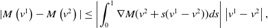
 $v(0) = \textbf{v}_0$
are illustrated in Figure 1a.
$v(0) = \textbf{v}_0$
are illustrated in Figure 1a.
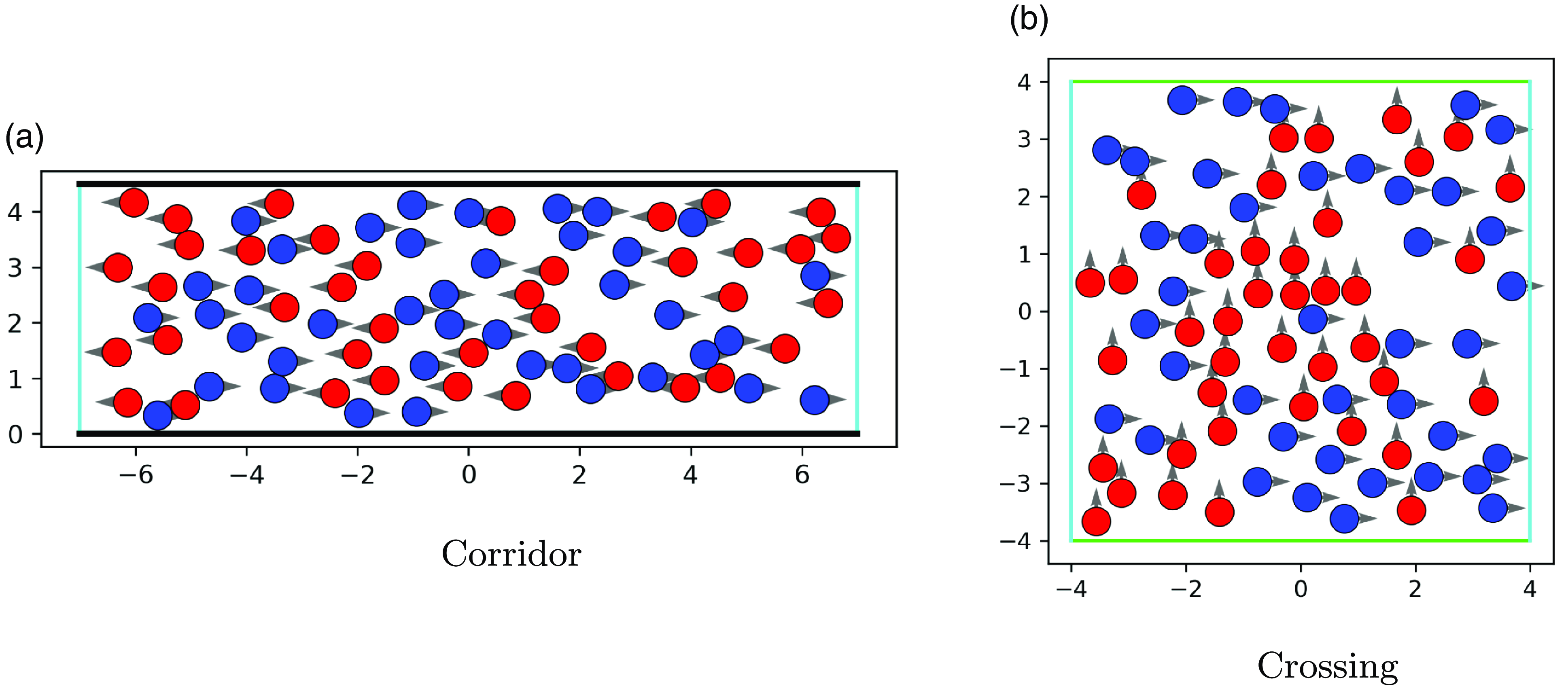
Figure 1. Initial positions and initial velocity vectors for the two scenarios with parameters $N=80,\ N_{\text{blue}} = 40, \ N_{\text{red}} = 40$
,
$N=80,\ N_{\text{blue}} = 40, \ N_{\text{red}} = 40$
, $d = 0.2$
.
$d = 0.2$
.
To assure that the pedestrians do not leave the scenario, we add reflective and periodic boundary conditions. In the corridor case the black lines (top and bottom) in Figure 1a show reflective boundaries. We model the avoidance of wall contact, by reflecting the velocity vector of an agent that would step outside of the domain in the next time step. The behavior of reflection from the wall is the same as in [Reference Totzeck34]. The light blue lines illustrate periodic boundaries. Blue agents leaving the domain at the boundary on the right, enter again from the left. Analogously for the red agents. With the periodic boundary condition, the number of agents in the system remains constant.
In the second scenario, we consider two groups of pedestrians at a crossing. Here, the blue group of pedestrians moves from left to right with desired velocity $w_{\text{blue}}=(0.7,0)^T$
, and the red group of pedestrians move from bottom to top with desired velocity
$w_{\text{blue}}=(0.7,0)^T$
, and the red group of pedestrians move from bottom to top with desired velocity $w_{\text{red}}=(0,0.7)^T$
. In total, there are
$w_{\text{red}}=(0,0.7)^T$
. In total, there are $N = N_{\text{blue}} + N_{\text{red}}$
pedestrians. The initial positions and initial velocity vectors are presented in Figure 1b. There, light blue and green lines represent periodic boundaries for blue and red agents, respectively. Altogether, this results in Algorithm 1 for the state system (2.1).
$N = N_{\text{blue}} + N_{\text{red}}$
pedestrians. The initial positions and initial velocity vectors are presented in Figure 1b. There, light blue and green lines represent periodic boundaries for blue and red agents, respectively. Altogether, this results in Algorithm 1 for the state system (2.1).
2.2.2. Study for different body sizes
To analyze the simulation results for different body sizes, we fix values for the force parameters and desired velocities of each pedestrian. The parameters are chosen to satisfy the stability ranges of the interaction force discussed in [Reference Degond, Appert-Rolland, Moussaid, Pettre and Theraulaz14]. In fact, in the range, $R/A \gt 1$
and
$R/A \gt 1$
and $r/a \lt 1$
the interaction force
$r/a \lt 1$
the interaction force $K$
is repulsive in the short range and attractive in the long range. This allows the distance between pedestrians to be maintained. Even if we include body size into the interaction force, it remains repulsive in a short-range and attractive in a long range. The strength of attraction and repulsion forces between agents ensures that they remain at a comfortable distance from each other and avoid collisions, regardless of their color. However, the overall direction of movement of the agents is primarily determined by their desired velocity
$K$
is repulsive in the short range and attractive in the long range. This allows the distance between pedestrians to be maintained. Even if we include body size into the interaction force, it remains repulsive in a short-range and attractive in a long range. The strength of attraction and repulsion forces between agents ensures that they remain at a comfortable distance from each other and avoid collisions, regardless of their color. However, the overall direction of movement of the agents is primarily determined by their desired velocity $w$
, which varies depending on the type of directed motion, such as bi-directional movement, crossing motion, crossing at an angle, and so on.
$w$
, which varies depending on the type of directed motion, such as bi-directional movement, crossing motion, crossing at an angle, and so on.
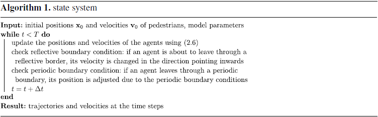
Figure 2 shows the simulation results of the corridor scenario for different body sizes. The results indicate a relation between the body size and the number of lanes formed. The smaller the body size, the more lanes are obtained. The parameters used for the simulation are reported in the caption of the figure. Similar results are found for the crossing scenario in Figure 3. Again, the smaller the body size, the more lanes are formed.
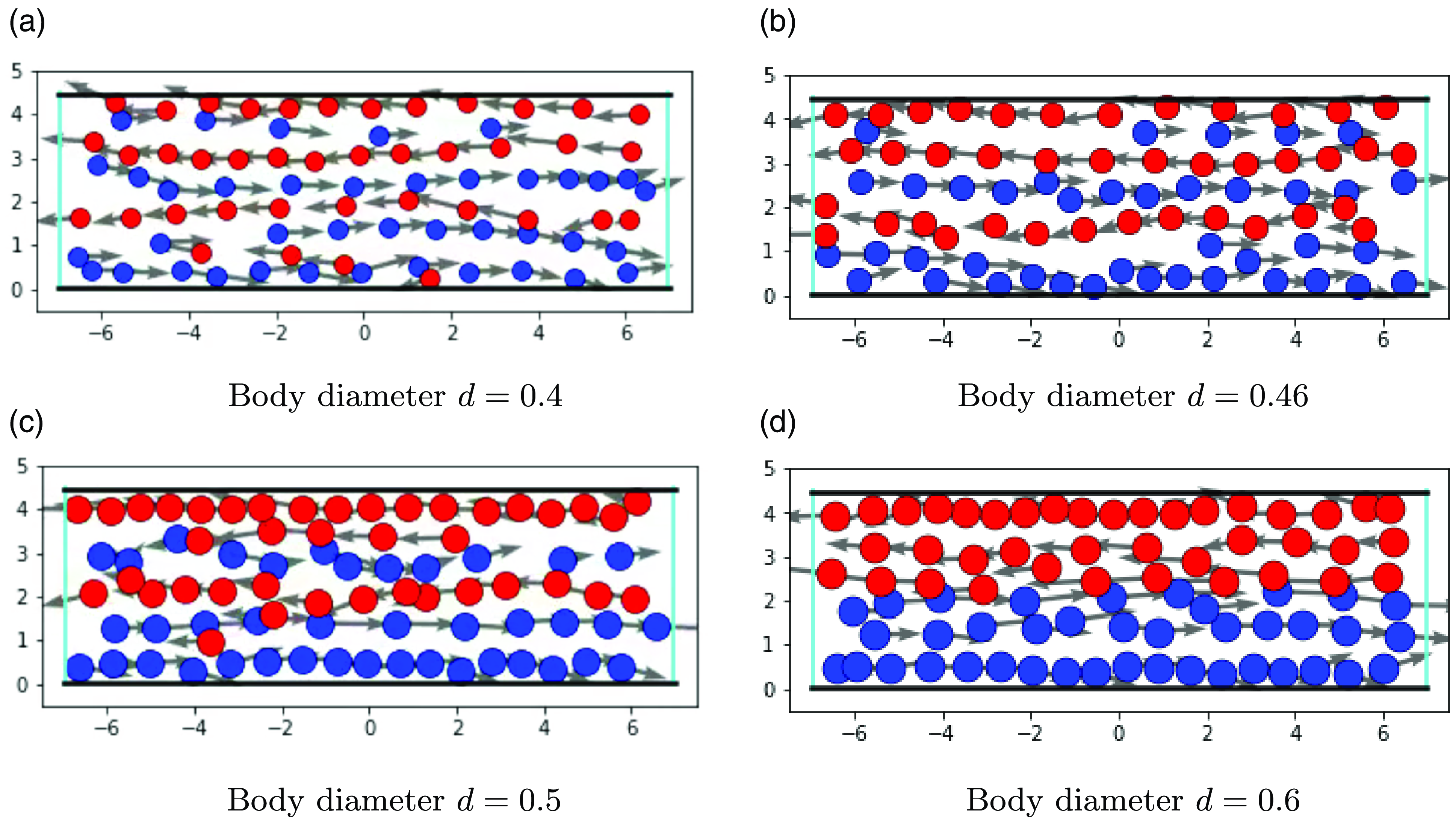
Figure 2. Simulation results in the corridor by different body sizes of pedestrians at time $T = 35$
. In each simulation, we fix parameters:
$T = 35$
. In each simulation, we fix parameters: $A=5, R=20, a=2, r=0.5, \lambda = 0.25$
. Desired velocities for red and blue agents are
$A=5, R=20, a=2, r=0.5, \lambda = 0.25$
. Desired velocities for red and blue agents are $w_{\text{red}}=({-}0.7, 0)^T$
and
$w_{\text{red}}=({-}0.7, 0)^T$
and $w_{\text{blue}}=(0.7, 0)^T$
, respectively. The time step in the Leap-Frog Scheme is
$w_{\text{blue}}=(0.7, 0)^T$
, respectively. The time step in the Leap-Frog Scheme is $\Delta t = 0.00625$
.
$\Delta t = 0.00625$
.
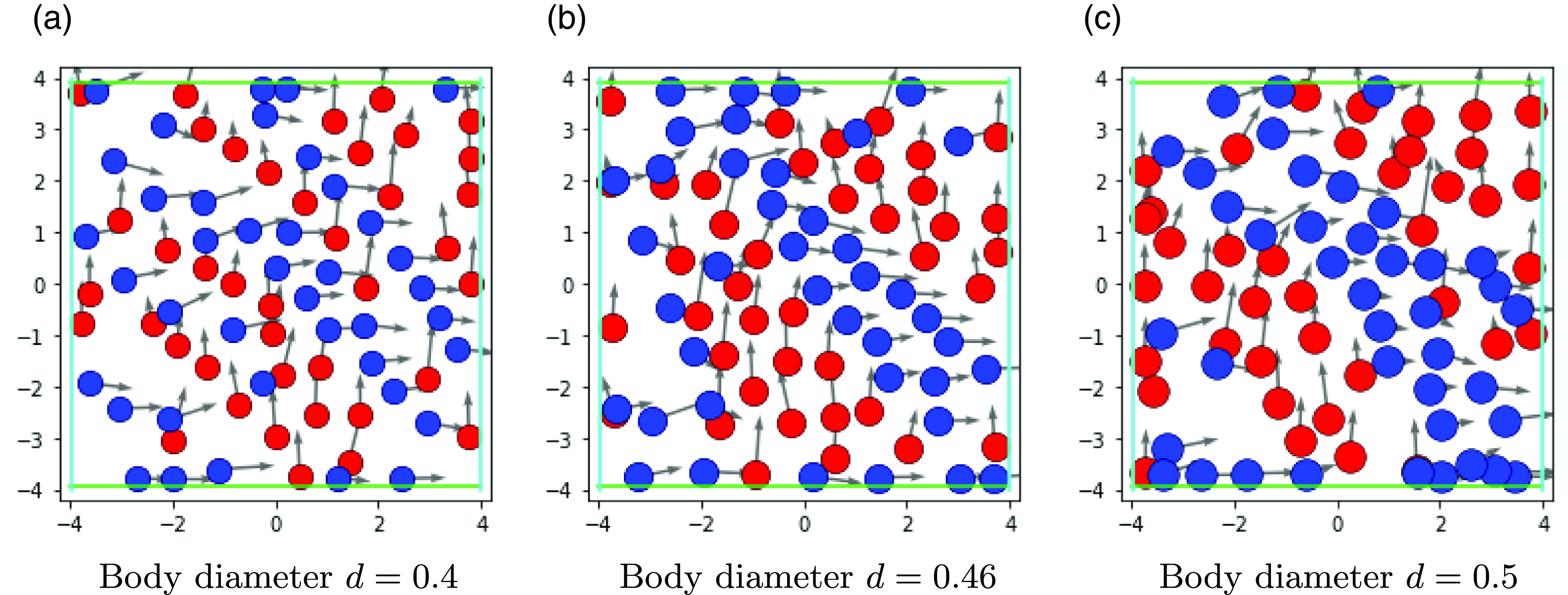
Figure 3. Simulation results at the crossing by different body sizes of pedestrians at time $T = 35$
. In each simulation, we fix parameters:
$T = 35$
. In each simulation, we fix parameters: $A=5, R=20, a=2, r=0.5, \lambda = 0.25$
. Desired velocities for red and blue agents are
$A=5, R=20, a=2, r=0.5, \lambda = 0.25$
. Desired velocities for red and blue agents are $\vec{w}_{\text{red}}=(0, 0.7)^T$
and
$\vec{w}_{\text{red}}=(0, 0.7)^T$
and $\vec{w}_{\text{blue}}=(0.7, 0)^T$
respectively. The time step in the leap-frog scheme is
$\vec{w}_{\text{blue}}=(0.7, 0)^T$
respectively. The time step in the leap-frog scheme is $\Delta t = 0.00625$
.
$\Delta t = 0.00625$
.
In all simulations, we see the formation of so-called traffic lanes. This formation seems to be independent of the choice of the random initial positions and velocities. It is interesting to note that even though every pedestrian is guided by simple rules for movement and interaction, phenomena arise that go beyond the behavior of single pedestrians. Such phenomena of self-organization are manifested in many multi-agent systems [Reference Helbing, Farkas, Molnar and Vicsek19]. They were reported in many articles concerning the movement of pedestrian flows [Reference Sieben, Schumann and Seyfried31, Reference Zhang, Zhu, Hostikka and Qiu36], which speaks in favor of the proposed model. Moreover, we want to emphasize that not only the body size can influence the number of lanes. In fact, the choice of the width of the corridor, the number of agents, and attraction and repulsion force parameters can change the formation of lanes as well. For the force parameters, this is shown exemplarily in Figure 4.

Figure 4. Simulation results in the corridor by different force parameters at time $T = 35$
. In each simulation, the body diameter of the agents is fixed:
$T = 35$
. In each simulation, the body diameter of the agents is fixed: $d=0.5$
. The time step in the leap-frog scheme is
$d=0.5$
. The time step in the leap-frog scheme is $\Delta t = 0.00625$
.
$\Delta t = 0.00625$
.
As the body size, the ratio of repulsion and attraction amplitudes, and the size of the corridor have similar effects in terms of volume exclusion, we suspect from these studies that volume exclusion is the main driver of the lane formation process.
2.2.3. Fundamental diagram
Often fundamental diagrams are employed to analyze crowd motion models [Reference Schadschneider, Klüpfel, Kretz, Rogsch and Seyfried27, Reference Zhang, Zhu, Hostikka and Qiu36]. Main objective is the relationship of speed and density [Reference Seyfried, Steffen, Klingsch and Boltes29, Reference Steffen and Seyfried32, Reference Zhang, Zhu, Hostikka and Qiu36] which we study for the bi-directional and crossing flow simulated with the model described in Section 2. For the illustration, we take the corridor with $17m$
length and
$17m$
length and $4m$
width, see Figure 5 for the bi-directional flow and the intersection of corridors with a width of
$4m$
width, see Figure 5 for the bi-directional flow and the intersection of corridors with a width of $4m$
and a length of
$4m$
and a length of $10m$
for the crossing flow, see Figure 6. The density approximation is realized with the help of Voronoi diagrams as proposed in [Reference Cao, Seyfried, Zhang, Holl and Song6, Reference Steffen and Seyfried32]. Initially, agents move with their desired walking speed until they slow down (or speed up) due to interaction forces. Most interactions take place in the center of the domain, it is therefore the focus of our interest.
$10m$
for the crossing flow, see Figure 6. The density approximation is realized with the help of Voronoi diagrams as proposed in [Reference Cao, Seyfried, Zhang, Holl and Song6, Reference Steffen and Seyfried32]. Initially, agents move with their desired walking speed until they slow down (or speed up) due to interaction forces. Most interactions take place in the center of the domain, it is therefore the focus of our interest.
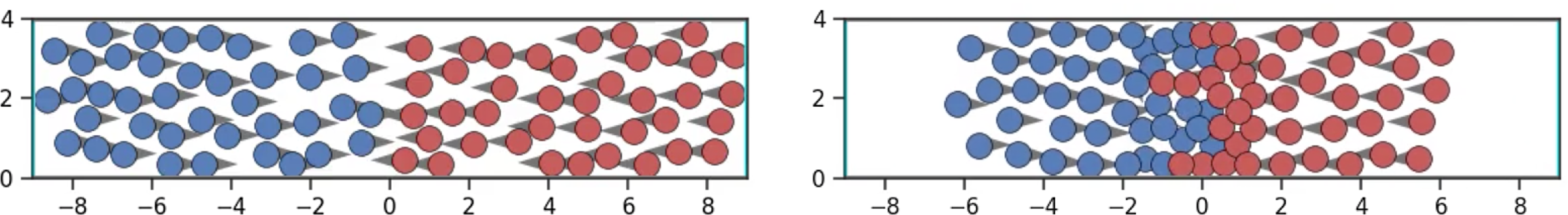
Figure 5. Bidirectional pedestrian flow at time $T=0$
and
$T=0$
and $T=5\,{\rm s}$
.
$T=5\,{\rm s}$
.

Figure 6. Crossing pedestrian flow at time $T=0$
and
$T=0$
and $T=4\,{\rm s}$
.
$T=4\,{\rm s}$
.
To approximate the density we construct Voronoi cells based on the positions of agents. The Voronoi diagram allows separating the area into computational grids (polygons) based on the triangulation of the computational area, in particular, the Delaunay triangulation [Reference Shewchuk30]. Every point on the Voronoi diagram has a region that is closer to it than any other [Reference Steffen and Seyfried32]. In Figure 7a we see Voronoi cells of all agents. Figure 7b shows the same cells, but only the ones in the region of interest $\Omega = [{-}2, 2]\times [0, 4]$
. For the crossing flow, the region of interest is
$\Omega = [{-}2, 2]\times [0, 4]$
. For the crossing flow, the region of interest is $\Omega = [{-}2, 2]\times [{-}2, 2]$
. Outside of the domain
$\Omega = [{-}2, 2]\times [{-}2, 2]$
. Outside of the domain $\Omega$
agents are involved in fewer interactions and walk approximately with their desired velocities. The model parameters in these simulation are set
$\Omega$
agents are involved in fewer interactions and walk approximately with their desired velocities. The model parameters in these simulation are set $\lambda =-0.07$
,
$\lambda =-0.07$
, $A = 6$
,
$A = 6$
, $R = 33$
,
$R = 33$
, $a=1$
,
$a=1$
, $r=0.3$
,
$r=0.3$
, $d=0.46$
. In the preceeding studies we focussed on the effect of the body size on the model dynamics. The magnitude of the parameter values was incidental. Now, we investigate whether the model is able to reproduce the fundamental diagram, which was found in many experimental studies. We therefore already use here the parameters obtained from the calibration in Section 3.
$d=0.46$
. In the preceeding studies we focussed on the effect of the body size on the model dynamics. The magnitude of the parameter values was incidental. Now, we investigate whether the model is able to reproduce the fundamental diagram, which was found in many experimental studies. We therefore already use here the parameters obtained from the calibration in Section 3.

Figure 7. Voronoi diagrams of bidirectional pedestrian flow at $T=5\,{\rm s}$
.
$T=5\,{\rm s}$
.
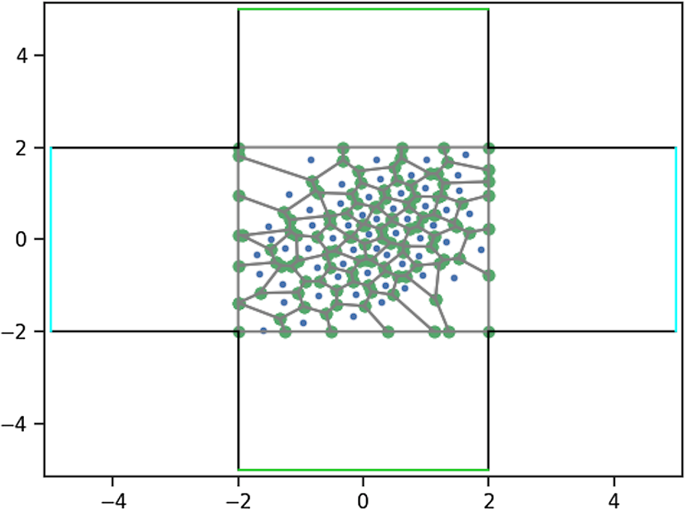
Figure 8. Bounded Voronoi diagram on $\Omega = [{-}2, 2]\times [{-}2, 2]$
of crossing pedestrian flow at
$\Omega = [{-}2, 2]\times [{-}2, 2]$
of crossing pedestrian flow at $T=5s$
.
$T=5s$
.
We employ the method proposed in [Reference Cao, Seyfried, Zhang, Holl and Song6, Reference Steffen and Seyfried32] to compute the density as follows
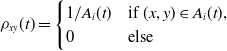 \begin{equation*} \rho _{xy} (t)= \begin {cases} 1/A_{i}(t) & \text{if}\ (x,y) \in A_{i}(t), \\ 0 & \text{else} \end {cases} \end{equation*}
where $A_i(t)$
gives the Voronoi cell area for agent
$A_i(t)$
gives the Voronoi cell area for agent $i$
, and
$i$
, and $\rho _{xy}$
is the density distribution of the space. Voronoi cells are computed using the Python, Scipy module, with the Voronoi and ConvexHull methods. Note that the velocities are given by the integration of (2.1).
$\rho _{xy}$
is the density distribution of the space. Voronoi cells are computed using the Python, Scipy module, with the Voronoi and ConvexHull methods. Note that the velocities are given by the integration of (2.1).
In Figure 9 we illustrate the relationship between density and speed at different time points. In the beginning, the agents move with the desired speed in regions with lower density leading to weak interaction forces. When the two groups meet, we see that as the density increases and at the same time the speed decreases as expected. Body size seems to have a minor influence on this effect.

Figure 9. Fundamental diagrams of pedestrian flow in the corridor and at the crossing scenario.
This ends our analysis and numerical study of the model. In the following sections, we are concerned with its parameter calibration based on real data [25]. We begin with the statement of the calibration problem and analyze its well-posedness.
3. Analysis of the parameter calibration problem
In this section, we state the parameter calibration problem and analyze the existence of minimizers. Then we lay the theoretical ground for the formulation of a gradient-descent method by deriving the first-order optimality conditions, the existence of adjoint states, and finally the identification of the gradient of the reduced cost functional. This prepares the formulation of a gradient descent-based calibration algorithm that will be employed in the numerical section to fit the parameters to real data from the BaSiGo experiment carried out in Düsseldorf in 2013 [Reference Cao, Seyfried, Zhang, Holl and Song6, 25] in the next section.
Let us begin with the statement of the parameter calibration problem. Table 1 shows all model parameters. For the calibration, we focus on the scaling factor $\lambda$
involved in the collision avoidance process and the force strengths
$\lambda$
involved in the collision avoidance process and the force strengths $A$
and
$A$
and $R$
and body size of agents
$R$
and body size of agents $d$
. We do not include the parameters
$d$
. We do not include the parameters $a$
and
$a$
and $r$
in the calibration problem, as the forces are driven by the ratios
$r$
in the calibration problem, as the forces are driven by the ratios $A/a$
as well as
$A/a$
as well as $R/r$
, hence increasing
$R/r$
, hence increasing $A,R$
or decreasing
$A,R$
or decreasing $a,r$
has similar effects. Numerical tests that included
$a,r$
has similar effects. Numerical tests that included $r,a$
in the calibration led to very unstable gradient behaviour, which we understood as a sign of overparameterization. We therefore fix
$r,a$
in the calibration led to very unstable gradient behaviour, which we understood as a sign of overparameterization. We therefore fix $r$
and
$r$
and $a$
for the following considerations.
$a$
for the following considerations.
Table 1. Model parameters
For fixed $1 \gg \epsilon \gt 0$
, we define the set of admissible parameters
$1 \gg \epsilon \gt 0$
, we define the set of admissible parameters
 \begin{equation*} U_{\text {ad}} = \Big \{(\lambda, A, R, d) \in [{-}1+\epsilon, 1-\epsilon ] \times [0,A_{\max }] \times [0,R_{\max }] \times [0, d_{\max }] \Big \} \end{equation*}
and we want to find ${u\,:\!=\, (\lambda, A, R, d)} \in U_{\text{ad}}$
such that the model trajectories fit the real trajectories best. We thus consider the cost functional
${u\,:\!=\, (\lambda, A, R, d)} \in U_{\text{ad}}$
such that the model trajectories fit the real trajectories best. We thus consider the cost functional
 \begin{equation*} J(x, u) \,:\!=\, \int _{0}^{T} \frac {\sigma _1}{2N} \sum _{i=1}^{N} \left \lVert x_{i}(t) - x_{i}^{\text {data}}(t)\right \rVert ^2_2 dt + \frac {\sigma _2}{2} \left \lVert u - u_{\text {ref}}\right \rVert ^2_2 \end{equation*}
with $x^{\text{data}}$
given trajectory data from experiments. The first term measures the distance of the trajectories resulting from the model to the real trajectories from the data. The second term of the cost functional penalizes the distance of the parameters to some given reference parameters
$x^{\text{data}}$
given trajectory data from experiments. The first term measures the distance of the trajectories resulting from the model to the real trajectories from the data. The second term of the cost functional penalizes the distance of the parameters to some given reference parameters $u_{\text{ref}}.$
In case there are no reference values available, we set
$u_{\text{ref}}.$
In case there are no reference values available, we set $\sigma _2 = 0.$
To study well-posedness, we use the following notion of optimality:
Definition 3.1.
We call $u \in U_{\text{ad}}$
optimal, if it is a solution to the optimization problem
$u \in U_{\text{ad}}$
optimal, if it is a solution to the optimization problem
 \begin{equation} \min _{(x,u) \in H^1([0,T], \mathbb{R}^{2N}) \times U_{ad}} J(x, u) \quad \quad \text{subject to} \, {(2.1)}. \end{equation}
Note that the calibration problem is constrained by the ODE system without boundary conditions. The boundary conditions are only incorporated in the numerical simulations to reflect the domain of the experiments appropriately.
In the following, we consider the spaces $Y$
and
$Y$
and $U$
given by
$U$
given by
 \begin{equation*} Y = \left[H^1\left([0,T], \mathbb {R}^{2N}\right) \times H^1\left([0,T], \mathbb {R}^{2N}\right) \right], \quad U = [{-}1,1] \times \mathbb {R} \times \mathbb {R} \times \mathbb {R}. \end{equation*}
Note that both, $Y$
and
$Y$
and $U$
are Hilbert spaces, and
$U$
are Hilbert spaces, and $U_{\text{ad}} \subset U$
is closed. For notational convenience we define the state vector
$U_{\text{ad}} \subset U$
is closed. For notational convenience we define the state vector $y=(x, v) \in Y$
and the state operator
$y=(x, v) \in Y$
and the state operator
 \begin{equation} e\,:\, Y \times U \rightarrow Z^*, \qquad e(y,u) = \begin{pmatrix} \frac{d}{dt} y- F(y,u) \\[5pt] y(0) - \textbf{y}_0 \end{pmatrix}, \end{equation}
where $F(y,u)$
is the vector containing the right-hand side of (2.1a) and (2.1b), respectively.
$F(y,u)$
is the vector containing the right-hand side of (2.1a) and (2.1b), respectively.
3.1. Well-posedness of the parameter calibration problem
The proof of the existence of an optimal parameter set for the calibration problem will be based on the following Lemmata which are concerned with the boundedness of the states with respect to the control parameters and the weak continuity of the state operator $e$
.
$e$
.
Lemma 3 (Boundedness). Let $w_i \in \mathcal C([0,T],{\mathbb{R}}^2)$
for all
$w_i \in \mathcal C([0,T],{\mathbb{R}}^2)$
for all $i=1,\dots,N$
and Assumption
1
hold and suppose the interaction forces are given by (2.5). For given
$i=1,\dots,N$
and Assumption
1
hold and suppose the interaction forces are given by (2.5). For given $u\in U_{\text{ad}}$
there exists a constant
$u\in U_{\text{ad}}$
there exists a constant $C\gt 0$
depending only on the body size
$C\gt 0$
depending only on the body size $d$
and
$d$
and
 \begin{equation*} \bar w \,:\!=\, \max \limits _{i} \sup \limits _{t\in [0,T]} \left \lVert w_i(t)\right \rVert,\end{equation*}
such that the solution $y\in Y$
with
$y\in Y$
with $e(y,u) = 0$
satisfies
$e(y,u) = 0$
satisfies
 \begin{equation*} \left \lVert y\right \rVert _Y \le C(1+ \left \lVert u\right \rVert ). \end{equation*}
Proof. We begin with the estimate for $\left \lVert y\right \rVert _{L^2([0,T],{\mathbb{R}}^2)}.$
It holds
$\left \lVert y\right \rVert _{L^2([0,T],{\mathbb{R}}^2)}.$
It holds
 \begin{equation*} \left \lVert x(t)\right \rVert ^2 \le 2\left \lVert x_0\right \rVert ^2+ 2\int _0^t \left \lVert v(s)\right \rVert ^2 ds, \ \ \left \lVert v(t)\right \rVert ^2 \le 2\left \lVert v_0\right \rVert ^2 + 2\int _0^t \left \lVert w(s) - v(s)\right \rVert ^2 + Ce^d \left \lVert u\right \rVert ^2 ds. \end{equation*}
Hence, using Gronwall Lemma we obtain $\left \lVert y(t)\right \rVert ^2 \le \left \lVert u\right \rVert ^2 e^{Ct}$
and integration over
$\left \lVert y(t)\right \rVert ^2 \le \left \lVert u\right \rVert ^2 e^{Ct}$
and integration over $[0,T]$
yields
$[0,T]$
yields $\left \lVert y\right \rVert _{L^2(0,T,{\mathbb{R}}^2)} \le C_1 \left \lVert u\right \rVert .$
For the time derivatives, we find
$\left \lVert y\right \rVert _{L^2(0,T,{\mathbb{R}}^2)} \le C_1 \left \lVert u\right \rVert .$
For the time derivatives, we find
 \begin{equation*} \left \lVert \frac {d}{dt} x(t)\right \rVert ^2 \le \left \lVert v(s)\right \rVert ^2, \qquad \left \lVert \frac {d}{dt} v(t)\right \rVert ^2 \le 2 \left \lVert w(s) - v(s)\right \rVert ^2 + 2Ce^d \left \lVert u\right \rVert ^2. \end{equation*}
Integration over $[0,T]$
leads to
$[0,T]$
leads to $\left \lVert \dfrac{d}{dt} y\right \rVert _{L^2(0,T,{\mathbb{R}}^2)} \le C(1 + \left \lVert u\right \rVert ).$
The two estimates together give the result.
$\left \lVert \dfrac{d}{dt} y\right \rVert _{L^2(0,T,{\mathbb{R}}^2)} \le C(1 + \left \lVert u\right \rVert ).$
The two estimates together give the result.
Lemma 4. Let Assumption 1 hold. The state operator
 \begin{equation*}e\,:\, Y \times U \rightarrow Z^*, \qquad e(y,u) = \begin {pmatrix} \frac {d}{dt} y- F(y,u) \\[5pt] y(0) - \textbf {y}_0 \end {pmatrix} \end{equation*}
is weakly continuous.
Proof. Let $(y_k,u_k) \rightharpoonup (\hat y, \hat u)$
as
$(y_k,u_k) \rightharpoonup (\hat y, \hat u)$
as $k\rightarrow \infty$
. We need to show that
$k\rightarrow \infty$
. We need to show that $e(y_k,u_k) \rightharpoonup e(\hat{y},\hat{u})$
as
$e(y_k,u_k) \rightharpoonup e(\hat{y},\hat{u})$
as $k\rightarrow \infty$
, which can be reformulated as follows.
$k\rightarrow \infty$
, which can be reformulated as follows.
For any given test function $\varphi \in \mathcal C_c^1(Z)$
, we need to obtain the following convergence property
$\varphi \in \mathcal C_c^1(Z)$
, we need to obtain the following convergence property
 \begin{equation*} \lim \limits _{k\rightarrow \infty } \int \langle e(y_k,u_k), \varphi \rangle dt \rightarrow \int \langle e(\hat {y},\hat {u}), \varphi \rangle dt. \end{equation*}
We estimate
 \begin{align*} &\lim \limits _{k\rightarrow \infty } \int _{0}^{t} \left [ \frac{d}{dt}y_k - \frac{d}{dt}\hat{y} - F(y_k,u_k) + F(\hat{y},\hat{u}) \right ] \varphi dt \\[5pt] &=: \lim \limits _{k\rightarrow \infty } \int _{0}^{t} \left [ \frac{d}{dt}y_k - \frac{d}{dt}\hat{y} \right ] \varphi dt \\[5pt] &\quad +\lim \limits _{k\rightarrow \infty } \int _{0}^{t} \begin{bmatrix} \hat{v} - v_k \\[5pt] \tau ({-} \hat{v} + v_k) - M_{\hat{\lambda }}(\hat{v}) K_{\hat A,\hat R}(\hat{d},\hat{x}) + M_{\lambda _k}(v_k) K_{A_k,R_k}(d_k,x_k) \end{bmatrix} \varphi dt \\[5pt] &= \lim \limits _{k\rightarrow \infty } \int _{0}^{t} \left [ \frac{d}{dt}y_k - \frac{d}{dt}\hat{y} \right ] \varphi dt +\lim \limits _{k\rightarrow \infty } \int _{0}^{t} \begin{bmatrix} -( v_k - \hat{v}) \\[5pt] \tau ( v_k - \hat{v}) \end{bmatrix} \varphi dt \\[5pt] &+ \lim \limits _{k\rightarrow \infty } \int _{0}^{t} \begin{bmatrix} 0\\[5pt] \big (M_{\lambda _k}(v_k) - M_{\hat \lambda }(\hat{v})\big ) K_{A_k,R_k}(d_k,x_k) + M_{\hat \lambda }(\hat{v}) \big ( K_{A_k,R_k}(d_k,x_k)- K_{\hat A,\hat R}(\hat{d},\hat{x}) \big )\end{bmatrix} \varphi dt \end{align*}
Clearly, the first and second integral tends to zero for $k\to \infty$
by the weak convergence of
$k\to \infty$
by the weak convergence of $y_k$
to
$y_k$
to $y \in Y$
.
$y \in Y$
.
Let us consider the third integral separately. We can estimate the first summand as
 \begin{align*} &\left \lVert M_{\lambda _k}(v_k) - M_{\hat \lambda }(\hat{v})\big ) K_{A_k,R_k}(d_k,x_k) \right \rVert \\[5pt] &\leq \left \lVert M_{\lambda _k}(v_k) - M_{\lambda _k}(\hat{v}) + M_{\lambda _k}(\hat{v}) - M_{\hat \lambda }(\hat{v})\big )\right \rVert \cdot \left \lVert K_{A_k,R_k}(d_k,x_k) \right \rVert \\[5pt] & \leq \left \lVert M_{\lambda _k}(v_k) - M_{\lambda _k}(\hat{v}) \right \rVert \cdot \left \lVert K_{A_k,R_k}(d_k,x_k) \right \rVert + \left \lVert M_{\lambda _k}(\hat{v}) - M_{\hat \lambda }(\hat{v})\big )\right \rVert \cdot \left \lVert K_{A_k,R_k}(d_k,x_k) \right \rVert \\[5pt] & \leq L_{\lambda _k} \left \lVert v_k - \hat{v}\right \rVert \cdot \left \lVert K_{A_k,R_k}(d_k,x_k) \right \rVert + \left \lVert M_{\lambda _k}(\hat{v}) - M_{\hat \lambda }(\hat{v})\big )\right \rVert \cdot \left \lVert K_{A_k,R_k}(d_k,x_k) \right \rVert. \end{align*}
From Lemma 1 we have $L_{\lambda _k}$
. We recall that
$L_{\lambda _k}$
. We recall that $K$
is Lipschitz continuous by Assumption 1, and that
$K$
is Lipschitz continuous by Assumption 1, and that $v_k$
is in
$v_k$
is in $H^1([0,T],{\mathbb{R}}^D) \hookrightarrow \hookrightarrow L^2([0,T],{\mathbb{R}}^D)$
. By weak convergence of
$H^1([0,T],{\mathbb{R}}^D) \hookrightarrow \hookrightarrow L^2([0,T],{\mathbb{R}}^D)$
. By weak convergence of $v_k \rightharpoonup \hat{v}$
and by this compact embedding, the first norm tends to zero as
$v_k \rightharpoonup \hat{v}$
and by this compact embedding, the first norm tends to zero as $k\to \infty$
. The
$k\to \infty$
. The $\left \lVert M_{\lambda _k}(\hat{v}) - M_{\hat \lambda }(\hat{v})\big )\right \rVert$
tends to zero by continuity of the map
$\left \lVert M_{\lambda _k}(\hat{v}) - M_{\hat \lambda }(\hat{v})\big )\right \rVert$
tends to zero by continuity of the map $\lambda \mapsto M_\lambda (v)$
.
$\lambda \mapsto M_\lambda (v)$
.
Analogously we obtain the convergence of the term $\left \lVert M_{\hat \lambda }(\hat{v}) \big ( K_{A_k,R_k}(d_k,x_k)- K_{\hat A,\hat R}(\hat{d},\hat{x}) \big )\right \rVert$
. Then, using continuity of the interaction force with respect to
$\left \lVert M_{\hat \lambda }(\hat{v}) \big ( K_{A_k,R_k}(d_k,x_k)- K_{\hat A,\hat R}(\hat{d},\hat{x}) \big )\right \rVert$
. Then, using continuity of the interaction force with respect to $A$
,
$A$
, $R$
and
$R$
and $d$
, and weak convergence of
$d$
, and weak convergence of $x_k \rightharpoonup \hat{x}$
and compact embedding
$x_k \rightharpoonup \hat{x}$
and compact embedding $x_k$
in
$x_k$
in $H^1([0,T],{\mathbb{R}}^D) \hookrightarrow \hookrightarrow L^2([0,T],{\mathbb{R}}^D)$
, we obtain the desired result.
$H^1([0,T],{\mathbb{R}}^D) \hookrightarrow \hookrightarrow L^2([0,T],{\mathbb{R}}^D)$
, we obtain the desired result.
Theorem 3.2.
There exists at least one solution $(y^*, u^*) \in Y \times U_{\text{ad}}$
to (P).
$(y^*, u^*) \in Y \times U_{\text{ad}}$
to (P).
Proof. The cost functional $J$
is bounded from below and the state system is well-posed, so there exists
$J$
is bounded from below and the state system is well-posed, so there exists
 \begin{equation*} m=\inf \limits _{(y,u) \in Y \times U_{\text{ad}} } J(y,u). \end{equation*}
Let $(u_{k}) \in U_{\text{ad}}$
be a minimizing sequence. The sequence
$(u_{k}) \in U_{\text{ad}}$
be a minimizing sequence. The sequence $(u_k) \subset U_{\text{ad}}$
is bounded, and by the reflexivity of
$(u_k) \subset U_{\text{ad}}$
is bounded, and by the reflexivity of $U$
it has a weakly convergent subsequence (not relabeled) with limit
$U$
it has a weakly convergent subsequence (not relabeled) with limit $\hat{u}$
. By Lemma 3 we obtain the boundedness of
$\hat{u}$
. By Lemma 3 we obtain the boundedness of $(y_k)$
and, again by reflexivity, the existence of
$(y_k)$
and, again by reflexivity, the existence of $\hat y$
such that
$\hat y$
such that
 \begin{equation} u_k \rightharpoonup \hat{u} \text{ in } U_{\text{ad}} \quad \text{and} \quad y_k \rightharpoonup \hat{y} \text{ in } Y \text{ as }k\rightarrow \infty. \end{equation}
The weak continuity of $e(y,u)$
shown in Lemma 4 implies
$e(y,u)$
shown in Lemma 4 implies
 \begin{equation*} \left \lVert e(\hat {y}, \hat {u}) \right \rVert \leq \liminf \limits _{k\rightarrow \infty } \left \lVert e(y_k,u_k) \right \rVert = 0. \end{equation*}
Hence $\hat y$
is the solution to the state equation with parameters
$\hat y$
is the solution to the state equation with parameters $\hat u.$
By the weak lower semi-continuity of the norm, we obtain
$\hat u.$
By the weak lower semi-continuity of the norm, we obtain
 \begin{equation*} J(\hat {y}, \hat {u}) \leq \liminf \limits _{k\rightarrow \infty } J(y_k,u_k) = m, \end{equation*}
which allows us to conclude that $(\hat{y}, \hat{u})$
is a minimizer of (P).
$(\hat{y}, \hat{u})$
is a minimizer of (P).
Remark 4. Because of the non-linearity of the state equation, we cannot expect the uniqueness of the optimal control.
Having the existence of an optimal solution, we proceed with the derivation of the first-order necessary conditions, which will form the basis of the identification algorithm.
3.2. First-order necessary conditions
We introduce the dual pairing
 \begin{align} \left \langle e(y, u), (\xi, \eta )\right \rangle _{Z, Z^*} =\int _{0}^{T} \left (\frac{d}{dt} y -F(y,u) \right ) \cdot \xi (t) dt+ (y(0)-\textbf{y}_0) \cdot \eta, \end{align}
where $\xi, \eta$
are the Lagrange multipliers in the Banach space
$\xi, \eta$
are the Lagrange multipliers in the Banach space
 \begin{equation*}Z = [L^2([0,T], \mathbb {R}^{2N}) \times L^2([0,T], \mathbb {R}^{2N}) \times \mathbb R^{2N} \times \mathbb R^{2N} ]\end{equation*}
that represent the space of the adjoint states. Here, $\xi = (\xi _x, \xi _v),$ $\eta = (\eta _x, \eta _v)$
and
$\eta = (\eta _x, \eta _v)$
and $(\xi, \eta ) \in Z$
. The space of states
$(\xi, \eta ) \in Z$
. The space of states $Y$
and the set of controls
$Y$
and the set of controls $U$
are defined at the beginning of Section 3.
$U$
are defined at the beginning of Section 3.
We formally derive the first-order optimality system with the help of the Lagrangian corresponding to the constrained parameter calibration problem given by
 \begin{equation} \mathcal{L}\,:\, Y\times U \times Z \rightarrow \mathbb{R}, \qquad \mathcal{L}(y, u, \xi, \eta ) = J(y, u) + \left \langle e(y, u), (\xi, \eta )\right \rangle _{Z, Z^*}. \end{equation}
3.2.1. Derivation of the adjoint system and the optimality condition
Solving $d \mathcal{L}(y, u, \xi, \eta ) = 0$
yields the first-order optimality condition [Reference Hinze, Pinnau, Ulbrich and Ulbrich21]. We begin with the computation of the directional derivatives of (3.4) with respect to the state
$d \mathcal{L}(y, u, \xi, \eta ) = 0$
yields the first-order optimality condition [Reference Hinze, Pinnau, Ulbrich and Ulbrich21]. We begin with the computation of the directional derivatives of (3.4) with respect to the state $y.$
For notational convenience we consider
$y.$
For notational convenience we consider $x$
and
$x$
and $v$
separately.
$v$
separately.
First, we obtain Gâteaux derivatives of the objective function
 \begin{equation*} d_{x_i} J(y, u)[h_{x_i}] = \frac {\sigma _1}{N} \int _{0}^{T} (x_{i}(t) -x_{i}^{data}(t) )h_{x_i} (t) dt,\qquad d_{v_i} J(y, u)[h_{v_i}] = 0. \end{equation*}
Now we derive the directional derivatives with respect to the positions of agents for the second part of the Lagrange functional
 \begin{align*} &d_{x_i}\left \langle e(y,u), (\xi, \eta )\right \rangle [h_{x_i}] =d_{x_i}\left \langle e_i(y,u), (\xi, \eta )_i\right \rangle [h_{x_i}] + \sum _{\substack{j=1\\j\neq i}}^{N}d_{x_i}\left \langle e_j(y,u), (\xi, \eta )_j\right \rangle [h_{x_i}]. \end{align*}
Using integration by parts, we obtain
 \begin{align} d_{x_i} \left \langle e(y,u), (\xi, \eta )\right \rangle [h_{x_i}] &= \int _{0}^{T} h_{x_i}^{\prime}\xi _{x_i}(t) + \frac{1}{N} h_{x_i} \sum _{\substack{j=1\\j\neq i}}^{N}\biggl (M(v_i,v_j)d_{x_i}K(x_i,x_j) \biggr )^T\xi _{v_i}(t) dt \\ &+ \int _{0}^{T} h_{x_i}\frac{1}{N} \sum _{\substack{j=1\\j\neq i}}^{N} \left [M(v_j,v_i) d_{x_i}K(x_j,x_i) \right ]^T\xi _{v_j}(t)dt + h_{x_i}(0)\eta _{x_i}.& \nonumber \end{align}
Since $M(v_i,v_j) = M(v_j,v_i)$
is symmetric and
$M(v_i,v_j) = M(v_j,v_i)$
is symmetric and $d_{x_i}K(x_i,x_j) = -d_{x_i}K(x_j,x_i)$
by the radial symmetry of
$d_{x_i}K(x_i,x_j) = -d_{x_i}K(x_j,x_i)$
by the radial symmetry of $K$
, we obtain
$K$
, we obtain
 \begin{align*} d_{x_i} \langle &e(y, u), (\xi, \eta )\rangle [h_{x_i}] = h_{x_i}(0)\eta _{x_i} \\ \qquad &+\int _{0}^{T} \biggl [ h_{x_i}^{\prime}(t)\xi _{x_i}(t) + h_{x_i}(t) \frac{1}{N} \sum _{\substack{j=1\\j\neq i}}^{N}\biggl (M(v_i,v_j)d_{x_i}K(x_i,x_j) \biggr )^T (\xi _{v_i}(t) - \xi _{v_j}(t)) \biggr ] dt. \end{align*}
Similarly, we obtain the derivative in direction $h_{v_i}.$
Indeed, by using integration by parts we find
$h_{v_i}.$
Indeed, by using integration by parts we find
 \begin{equation} d_{v_i}\left \langle e(y, u), (\xi, \eta )\right \rangle [h_{v_i}] =d_{v_i}\left \langle e_i(y, u), (\xi, \eta )_i\right \rangle [h_{v_i}] + \sum _{\substack{j=1\\j\neq i}}^{N}d_{v_i}\left \langle e_j(y, u), (\xi, \eta )_j\right \rangle [h_{v_i}]. \end{equation}
To simplify the notation we introduce the operator $d_{v_i}M^*(v_i,v_j)$
resulting from matrix reformulations, see Appendix B for more details. We get
$d_{v_i}M^*(v_i,v_j)$
resulting from matrix reformulations, see Appendix B for more details. We get
 \begin{align*} d_{v_i}\langle e(y, u), (\xi, \eta )\rangle [h_{v_i}] = &h_{v_i}(0)\eta _{v_i} + \int _{0}^{T} h_{v_i}^{\prime}\xi _{v_i}(t) - h_{v_i}\xi _{x_i}(t) + \tau h_{v_i}\xi _{v_i}(t)\; dt \\ &+ \int _{0}^{T} h_{v_i} \biggl [ \frac{1}{N} \sum _{\substack{j=1\\j\neq i}}^{N}d_{v_i} M^*(v_i,v_j) K(x_i,x_j) \xi _{v_i}(t)\\ &+ \frac{1}{N}\sum _{\substack{j=1\\j\neq i}}^{N} d_{v_i}M^*(v_j,v_i) K(x_j,x_i)\xi _{v_j}(t) \biggr ] dt. \end{align*}
Moreover, the directional derivatives with respect to the control are given by
 \begin{align} d_u J(y, u)[h_u] = \sigma _2 (u -u_{ref})h_{u}, \end{align}
 \begin{align} d_{u}\left \langle e(y, u), (\xi, \eta )\right \rangle [h_{u}] = -\int _{0}^{T} h_{u} \sum _{i} \left [d_{u} F(y_i,u)\right ]^T \xi _{v_i}(t)dt. \end{align}
Remark 5. For the specific choice (2.5), as we choose the interaction forces for the numerical results, the derivatives read
 \begin{align*} &\frac{dF(y_i,u) }{d\lambda } = \begin{cases} -\frac{1}{N} \sum \limits _{j \neq i} \begin{pmatrix} -\sin \alpha _{ij} & \quad -\cos \alpha _{ij} \\[3pt] \cos \alpha _{ij} & \quad -\sin \alpha _{ij} \end{pmatrix} \arccos \frac{v_i \cdot v_j}{\left \lVert v_i\right \rVert \left \lVert v_j\right \rVert } \cdot K(x_i, x_j), & \text{for } v_i, v_j \neq 0, \\ \\ \vec{0}_{2\times 1}, & \text{else} \end{cases},&\\ &\frac{dF(y_i,u) }{dA} = -\frac{1}{a\cdot N} \sum _{j\neq i} M(v_i,v_j) \cdot e^{\frac{d-\left \lVert x_i-x_j\right \rVert }{a}} \cdot \frac{x_i - x_j}{\left \lVert x_i-x_j\right \rVert },&\\ &\frac{dF(y_i,u) }{dR} = \frac{1}{r\cdot N} \sum _{j\neq i} M(v_i,v_j) \cdot e^{\frac{d-\left \lVert x_i-x_j\right \rVert }{r}} \cdot \frac{x_i - x_j}{\left \lVert x_i-x_j\right \rVert }.&\\ & \frac{dF(y_i,u) }{dd} = -\frac{1}{N} \sum _{j\neq i} M(v_i,v_j) \cdot \left (\frac{A}{a^2} e^{\frac{d-\left \lVert x_i-x_j\right \rVert }{a}} - \frac{R}{r^2}e^{\frac{d-\left \lVert x_i-x_j\right \rVert }{r}}\right ) \cdot \frac{x_i - x_j}{\left \lVert x_i-x_j\right \rVert }.& \end{align*}
3.2.2. Existence of adjoint states
The proof of the existence of adjoint states is based on Corollary 1.3 in [Reference Hinze, Pinnau, Ulbrich and Ulbrich21], which we give in Appendix C for completeness.
Theorem 3.3.
Let $w_i \in \mathcal C([0,T],{\mathbb{R}}^2), i=1,\dots,N$
be given, the Assumption
1
and
2
hold and
$w_i \in \mathcal C([0,T],{\mathbb{R}}^2), i=1,\dots,N$
be given, the Assumption
1
and
2
hold and $u^* \in U_{\text{ad}}$
be an optimal solution of Problem (
P
) and let
$u^* \in U_{\text{ad}}$
be an optimal solution of Problem (
P
) and let $y^* \in Y$
such that
$y^* \in Y$
such that $e(y^*,u^*)=0$
. Then there exist an adjoint state
$e(y^*,u^*)=0$
. Then there exist an adjoint state $p^*=(\xi ^{*}, \eta ^*) \in Z^*$
such that the following optimality conditions hold
$p^*=(\xi ^{*}, \eta ^*) \in Z^*$
such that the following optimality conditions hold
 \begin{align*} &\langle e(y^*,u^*), p \rangle _{Z,Z^*} = 0 &&\forall p \in Z^*, \\ &\langle L_y(y^*, u^*,p^*), h \rangle _{Y^*,Y} = 0 &&\forall h \in Y^*, \\ &u^* \in U_{\text{ad}}, \langle L_u(y^*, u^*, p^*), u-u^* \rangle _{U^*,U} \ge 0, &&\forall u\in U_{\text{ad}}. \end{align*}
Proof. We check requirements given in Assumption 3 (see Appendix C):
-
(A1) $ U_{\text{ad}} = [{-}1+\epsilon, 1-\epsilon ] \times [0,A_{\max }] \times [0,R_{\max }] \times [0,d_{\max }] \subset U$
is nonempty, convex and closed.
$ U_{\text{ad}} = [{-}1+\epsilon, 1-\epsilon ] \times [0,A_{\max }] \times [0,R_{\max }] \times [0,d_{\max }] \subset U$
is nonempty, convex and closed. -
(A2) We first note that
$U,Y,Z$
are Banach spaces. Further,
$J$
is of tracking type and therefore Fréchet differentiable [Reference Tröltzsch35]. We are left to show Fréchet differentiability of the state operator
$e(y,u)\,:\, Y \times U \rightarrow Z.$
In Section 3.2.1 we computed the first variations of
$e(y,u)$
with respect to
$y$
and
$u$
byand obtained (3.5) and (3.6). There, the continuity of linear terms follows directly from the definition. We show the continuity for nonlinear terms:
\begin{equation*} d_{y} \left \langle e(y, u)[(h_y)], (\xi, \eta )\right \rangle = \lim \limits _{\epsilon \rightarrow 0} \frac {1}{\epsilon }\left \langle e(y+\epsilon h_y, u) - e(y,u), (\xi, \eta )\right \rangle, \end{equation*}
Let, the sequence
$y_k\,:\!=\,(x_k, v_k) \subset Y$
have the limit
$y_k$
such that
$x_k \rightarrow x \text{ and } v_k \rightarrow v$
as
$k \rightarrow \infty$
. Using Assumption 2 we show the continuity of nonlinear terms in (3.5). Indeed, for the
$i$
-th component, it holdswhere
\begin{align*} &\int _{0}^{T} \frac{1}{N} h_{x_i} \sum _{\substack{j=1\\j\neq i}}^{N}\biggl (M(v_{k_i},v_{k_j})d_{x_i}K(x_{k_i},x_{k_j}) - M(v_i,v_j)d_{x_i}K(x_i,x_j) \biggr )^T\ \left (\xi _{v_i}- \xi _{v_j}\right )dt \\ &\leq L_1\cdot L_2 \int _{0}^{T} \frac{1}{N}\sum _{\substack{j=1\\j\neq i}}^{N}\biggl ( \left \lVert v_{k_i} - v_i\right \rVert + \left \lVert v_{k_j} - v_j\right \rVert + \left \lVert x_{k_i} - x_i\right \rVert \\ &\qquad \qquad \qquad + \left \lVert x_{k_j} - x_j\right \rVert \biggr )\left \lVert \xi _{v_i} - \xi _{v_j}\right \rVert dt \leq L_1 \cdot L_2 \int _{0}^{T} \left \lVert y_{k_i} - y_i\right \rVert \left \lVert \xi _{v_i} - \xi _{v_j}\right \rVert dt, \end{align*}
$L_1, L_2$
are Lipschitz constants. Analogously, we show the continuity for the nonlinear terms of (3.6) using Assumption 1 and Appendix A. These, yield the continuity of the state operator
$e(y,u)$
by
$y$
. The continuity with respect to
$u$
, can be concluded from the continuity of the
$\lambda \mapsto M,$
and the linearity of the force term with respect to
$A$
and
$R$
. Altogether, this proves the continuity of
$e$
as desired.
-
(A3) By Lemma 2 the state system
$e(y,u) = 0$
has an unique solution
$y=y(u) \in Y$
for all
$u \in V \subset U$
a neighborhood of
$U_{\text{ad}}.$
-
(A4) We have to show that
$e_y(y(u), u) \in \mathcal{L}(Y,Z)$
has a bounded inverse for all
$u \in V \supset U_{\text{ad}}$
. We can write
$d_{y}e(y, u)[h]$
in general formwhere
\begin{equation*}d_{y}e(y, u)[h] = \frac {d}{dt}h(t) + d_yF(y, u)h(t),\end{equation*}
$d_yF(y, u)$
is integrable in
$t$
over every finite interval
$I \subset [0,T]$
thanks to Assumption 2. We consider
$d_{y}e(y, u)[h] = r$
for arbitrary
$r\in Z^*.$
By Carathéodory’s existence theorem, we get for every
$r \in Z^*$
a unique solution [Reference Fornasier and Solombrino16], namely
$h=d_y e(y,u)^{-1}[r]$
. Using
$d_{y}e(y(u), u)$
, we obtainand with the help of Gronwall’s Lemma, we get the boundedness of the inverse of
\begin{equation*} \left \lVert h(t)\right \rVert \leq \left \lVert h(0)\right \rVert + \int _{0}^{T} \left \lVert r(s)\right \rVert ds +C\exp {\left (\int _{0}^{T}\left \lVert h(s)\right \rVert ds\right )}, \quad t\in [0,T] \end{equation*}
$d_{y}e(y(u), u)$
.


Altogether, the requirements of Assumption 3 are satisfied, and thus Proposition 1 (see Appendix C) yields the existence of an adjoint state.
Remark 6.
Note that assuming more regularity of the adjoint states, for instance, $Z=Y$
, we may establish the strong formulation of the adjoint system given by
$Z=Y$
, we may establish the strong formulation of the adjoint system given by
 \begin{align} \xi ^{\prime}_{x_i}(t) = & \frac{\sigma _1}{N} (x_{i}(t) - x_{i}^{data}(t)) + \frac{1}{N} \sum _{\substack{j=1\\j\neq i}}^{N}\biggl (M(v_i,v_j)d_{x_i}K(x_i,x_j)\biggr )^T(\xi _{v_i}(t) - \xi _{v_j}(t)), \nonumber \\ \xi ^{\prime}_{v_i}(t) = &-\xi _{x_i}(t) + \tau \xi _{v_i}(t) - \frac{1}{N} \sum _{\substack{j=1\\j\neq i}}^{N} d_{v_i} M^*(v_i,v_j)K(x_i,x_j) \xi _{v_i}(t) \nonumber \\ &- \frac{1}{N} \sum _{\substack{j=1\\j\neq i}}^{N} d_{v_i} M^*(v_j(t),v_i(t))K(x_j(t),x_i(t)) \xi _{v_j}(t)& \end{align}
supplemented with the terminal conditions $ \xi _{x_i}(T) =0, \ \xi _{v_i}(T) =0.$
The strong form will be employed for the numerical results in Section
4
.
$ \xi _{x_i}(T) =0, \ \xi _{v_i}(T) =0.$
The strong form will be employed for the numerical results in Section
4
.
3.2.3. Gradient of the reduced cost functional
To minimize the objective function we aim to apply a gradient descent algorithm. In order to determine the gradient, we define the control-to-state operator $ \mathcal{F}\,:\, U \rightarrow Y$
, and introduce the reduced cost functional as
$ \mathcal{F}\,:\, U \rightarrow Y$
, and introduce the reduced cost functional as $\hat{J}(u)\,:\!=\, J(\mathcal{F}(u), u)$
. Using
$\hat{J}(u)\,:\!=\, J(\mathcal{F}(u), u)$
. Using $e(y,u) = 0$
, we obtain
$e(y,u) = 0$
, we obtain
 \begin{equation*} 0=d_{y}e(\mathcal {F}(u), u)[d\mathcal {F}(u)] + d_{u} e(\mathcal {F}(u),u). \end{equation*}
Taking the derivative of the Lagrangian with respect to the state $y$
, we get
$y$
, we get
 \begin{equation*} d_{y}e(y,u)^{*}\xi = -d_{y}J(y,u). \end{equation*}
With these, we can compute the Gâteaux derivative of the reduced cost functional in the direction $h_{u} \in U$
, and obtain
$h_{u} \in U$
, and obtain
 \begin{align*} d\hat{J}(u)[h_{u}] &= \langle d_{y}J(y,u), d\mathcal{F}(u)[h_{u}] \rangle + \langle d_{u}J(y,u),h_{u}\rangle \\ &= \langle d_{u}e(y,u)^{*}\xi, h_{u} \rangle + \langle d_{u}J(y,u), h_{u}\rangle = d_{u}\mathcal{L}(y,u,\xi )[h_u].& \end{align*}
Note that we have already computed $ d_{u}J(y,u)$
in Section 3.2.1. This allows us to identify the gradient of the reduced cost functional as
$ d_{u}J(y,u)$
in Section 3.2.1. This allows us to identify the gradient of the reduced cost functional as
 \begin{align} \nabla \hat{J}(u) = \sigma _2 (u -u_{ref}) -\int _{0}^{T} \sum _{i} \left [d_{u} F(y_i,u)\right ]^T \xi _{v_i}(t)dt. \end{align}
4. Calibration algorithm and results
To calibrate the control parameters we use real data from the BaSiGo experiment carried out in Düsseldorf in 2013 [Reference Cao, Seyfried, Zhang, Holl and Song6, 25]. In the following, we denote the trajectories from experimental data by $x_{i}^{\text{data}}\,:\,[0,T] \rightarrow \mathbb{R}^2,{i=1\dots N}.$
For the corridor case, we take the data from file ”bi_corr_400_a_02.txt” in [25]. These show the positions of the pedestrians in the domain
$x_{i}^{\text{data}}\,:\,[0,T] \rightarrow \mathbb{R}^2,{i=1\dots N}.$
For the corridor case, we take the data from file ”bi_corr_400_a_02.txt” in [25]. These show the positions of the pedestrians in the domain $\Omega = [{-}6, 6]\times [0, 4.2],$
over time
$\Omega = [{-}6, 6]\times [0, 4.2],$
over time $t \in [0, 150]$
seconds. For the crossing case, we take the data from file “CROSSING_90_E_2.txt” in [25]. This file provides the positions of the pedestrians in the crossing corridors
$t \in [0, 150]$
seconds. For the crossing case, we take the data from file “CROSSING_90_E_2.txt” in [25]. This file provides the positions of the pedestrians in the crossing corridors $\Omega ={([{-}5, 5]\times [{-}1.5, 2])\cap ([{-}1.2, 2]\times [{-}5, 5])},$
over time
$\Omega ={([{-}5, 5]\times [{-}1.5, 2])\cap ([{-}1.2, 2]\times [{-}5, 5])},$
over time $t \in [0, 283]$
seconds. However, in the calibration algorithm, we use only 8-second intervals for both scenarios. In this way we can extract several batches from one movie and are computationally efficient. Moreover, once the model deviates from the data, cost will accumulate over time. By working with small time intervals this error is reduced. However, we also tested longer simulations times which led to similar results.
$t \in [0, 283]$
seconds. However, in the calibration algorithm, we use only 8-second intervals for both scenarios. In this way we can extract several batches from one movie and are computationally efficient. Moreover, once the model deviates from the data, cost will accumulate over time. By working with small time intervals this error is reduced. However, we also tested longer simulations times which led to similar results.
4.1. Numerical schemes and steepest descent algorithm
In general, the nonlinearities make it rather difficult to solve the optimality system all at once. We, therefore, opt for an iterative approach to compute the gradient of the calibration problem. Indeed, we first solve the state system (2.1) as considered in Section 2.1.1. Then, we integrate the adjoint system (3.9) with the help of a second-order Runge-Kutta method backward in time. Here, we use the same time steps as for the state problem and transform the time via $s=T-t$
to recover an initial value problem. With the state solution and the adjoint solution, we calculate the gradient using (3.10), where the integral is approximated with the trapezoidal rule.
$s=T-t$
to recover an initial value problem. With the state solution and the adjoint solution, we calculate the gradient using (3.10), where the integral is approximated with the trapezoidal rule.
We apply a steepest descent algorithm to update the control parameters in every iteration
 \begin{align} u^{k+1} = u^{k} - \beta _k \cdot \nabla \hat{J}(u) \end{align}
where $u^{k}$
denotes the control on current time step, and
$u^{k}$
denotes the control on current time step, and $\nabla \hat{J}(u)$
denotes the descent direction and
$\nabla \hat{J}(u)$
denotes the descent direction and $\beta _k \in{\mathbb{R}}^4$
is a positive scaling vector. The complete optimization procedure is summarized in Algorithm 2.
$\beta _k \in{\mathbb{R}}^4$
is a positive scaling vector. The complete optimization procedure is summarized in Algorithm 2.
Since we cannot assume that the data and the model are a perfect match, we employ a stochastic gradient descent approach using mini-batches [Reference Li, Zhang, Chen and Smola24]. To obtain the mini-batches from the data trajectories which are given on the interval $[0,T]$
, we split the interval into
$[0,T]$
, we split the interval into $M$
mini-batches, each of size
$M$
mini-batches, each of size $b_i = T/M$
,
$b_i = T/M$
, $i=1 \dots M$
. Then we randomly select
$i=1 \dots M$
. Then we randomly select $m\lt M$
mini-batches for each of the gradient steps.
$m\lt M$
mini-batches for each of the gradient steps.
In more detail, at each iteration we compute the gradients of the $m$
batches and approximate the gradient using the average
$m$
batches and approximate the gradient using the average
 \begin{equation*} { \nabla \hat {J}(u) = \frac {1}{m} \sum _{i=1}^{m} \nabla \hat {J}_{b_i}(u) } \end{equation*}
to update the control via (4.1). The stopping criterion of the calibration algorithm is based on the relative error between the previous and current cost function value denoted by $\epsilon _{\text{rel}}.$
4.2. Numerical results
In this section, we discuss numerical results generated with Algorithm 2 using experimental data from the Pedestrian Dynamics Data Archive [25]. In particular, we retrieve the trajectories from video recordings showing bi-directional and cross-directional flows.
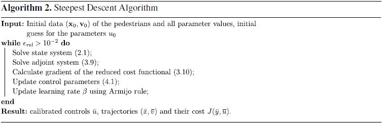
We fix the velocity scaling $\tau = 1$
, attractive potential range
$\tau = 1$
, attractive potential range $a=1$
, repulsive potential range
$a=1$
, repulsive potential range $r=0.3$
. The total number of pedestrians presented in the data is
$r=0.3$
. The total number of pedestrians presented in the data is $N=84$
in the corridor case and
$N=84$
in the corridor case and $N=71$
in the crossing scenario. The desired velocities of agents that go from right to left and from left to right are respectively
$N=71$
in the crossing scenario. The desired velocities of agents that go from right to left and from left to right are respectively $w_{\text{red}} = ({-}0.7, 0)^T$
and
$w_{\text{red}} = ({-}0.7, 0)^T$
and $w_{\text{blue}}=(0.7, 0)^T$
. The value
$w_{\text{blue}}=(0.7, 0)^T$
. The value $0.7$
is the average velocity that we extracted from the experimental data. The desired velocities for the crossing scenario are again computed from the experimental data and set to
$0.7$
is the average velocity that we extracted from the experimental data. The desired velocities for the crossing scenario are again computed from the experimental data and set to $w_{\text{red}} = (0, 1.2)^T$
and
$w_{\text{red}} = (0, 1.2)^T$
and $w_{\text{blue}}=(1.2, 0)^T$
. It is interesting that in the crossing scenario agents move faster than agents in the corridor. However, from the video data of the crossing scenario, we see that in the interacting part of the domain are fewer people. Also, in the corridor case, agents try to move alongside the whole corridor avoiding collisions, while in the crossing case, agents interact just on the crossroad.
$w_{\text{blue}}=(1.2, 0)^T$
. It is interesting that in the crossing scenario agents move faster than agents in the corridor. However, from the video data of the crossing scenario, we see that in the interacting part of the domain are fewer people. Also, in the corridor case, agents try to move alongside the whole corridor avoiding collisions, while in the crossing case, agents interact just on the crossroad.
The time step in the Leap Frog scheme and second order Runge-Kutta method is set to $\Delta t = 0.00625$
. Simulations are done in the time interval
$\Delta t = 0.00625$
. Simulations are done in the time interval $t\in [0,8]$
. The gradient is calculated with
$t\in [0,8]$
. The gradient is calculated with $m = 50$
mini-batches of length
$m = 50$
mini-batches of length $|b_{i}| =10\cdot \Delta t$
. The short mini-batch length can lead to a non-smooth decrease in the cost function.
$|b_{i}| =10\cdot \Delta t$
. The short mini-batch length can lead to a non-smooth decrease in the cost function.
The initial positions of the agents $\textbf x_0$
coincide with the initial positions of the experimental data, which are distributed in the domain
$\textbf x_0$
coincide with the initial positions of the experimental data, which are distributed in the domain $[{-}6,6]\times [0,4.2]$
. As the initial velocity of the pedestrians, we set the average velocity from the experimental data. We probably induce some error here, as we do not have the exact values from the data.
$[{-}6,6]\times [0,4.2]$
. As the initial velocity of the pedestrians, we set the average velocity from the experimental data. We probably induce some error here, as we do not have the exact values from the data.
As an initial guess of the control parameters, we take $u_0=(0, 0, 40, 0.6)$
for both experiments. We set the regularization parameters in the cost functional to
$u_0=(0, 0, 40, 0.6)$
for both experiments. We set the regularization parameters in the cost functional to $\sigma _1 = 1$
and
$\sigma _1 = 1$
and $\sigma _2 = 0$
. We, therefore, do not need to choose reference values for the control. In this setting, we repeat Algorithm 2 while the given stopping criterion is fulfilled. As the interval length of the mini-batches is rather short, the magnitude of the gradient compontens is rather small. We therefore multiply with a step size parameter
$\sigma _2 = 0$
. We, therefore, do not need to choose reference values for the control. In this setting, we repeat Algorithm 2 while the given stopping criterion is fulfilled. As the interval length of the mini-batches is rather short, the magnitude of the gradient compontens is rather small. We therefore multiply with a step size parameter $\beta$
which accounts for the different ranges of the control values. This can be seen as a kind of preconditioning. The initial step size parameter
$\beta$
which accounts for the different ranges of the control values. This can be seen as a kind of preconditioning. The initial step size parameter $\beta _0 = (20, 4000, 4000, 20)$
was found by trial and error. Further, we change
$\beta _0 = (20, 4000, 4000, 20)$
was found by trial and error. Further, we change $\beta _k$
using the Armijo rule. The Armijo rule ensures a sufficient decrease in the objective function.
$\beta _k$
using the Armijo rule. The Armijo rule ensures a sufficient decrease in the objective function.
Figure 10a illustrates the decrease of the cost functional for the corridor case with initial body diameter $d=0.6$
. It starts from approximately 6.53 in the first iteration and terminates at around 5.14 in the last iteration. In Figure 10b we see the evolution of the cost for the crossing scenario from 8.83 to 7.46. We note that the cost values of the corridor are smaller than the ones of the crossing case. This indicates that the proposed model captures the effects of counter-flow better than the effects of crossing flow.
$d=0.6$
. It starts from approximately 6.53 in the first iteration and terminates at around 5.14 in the last iteration. In Figure 10b we see the evolution of the cost for the crossing scenario from 8.83 to 7.46. We note that the cost values of the corridor are smaller than the ones of the crossing case. This indicates that the proposed model captures the effects of counter-flow better than the effects of crossing flow.
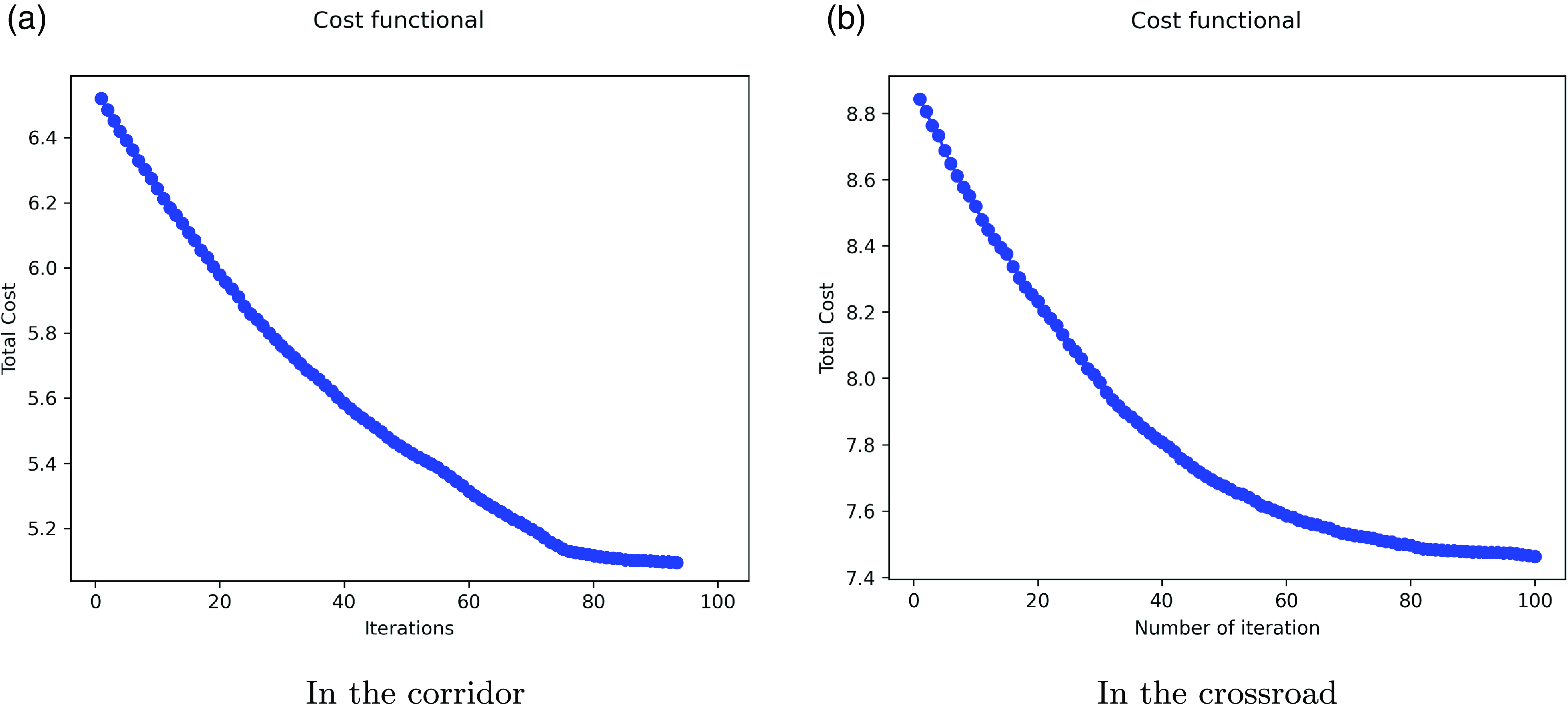
Figure 10. Cost functionals of the corridor and crossing scenarios.
In Table 2 the calibration results with different body size are presented. The parameters of the first calibration procedure reached optimal values $\lambda = -0.072$
,
$\lambda = -0.072$
, $A = 6.14$
,
$A = 6.14$
, $R=33.29$
, and
$R=33.29$
, and $d=0.46$
for the simulation in the corridor. For the simulation at the crossing scenario, optimal values reached
$d=0.46$
for the simulation in the corridor. For the simulation at the crossing scenario, optimal values reached $\lambda = -0.068$
,
$\lambda = -0.068$
, $A = 8.66$
,
$A = 8.66$
, $R=32.91$
, and
$R=32.91$
, and $d = 0.456$
. Interestingly, the optimal
$d = 0.456$
. Interestingly, the optimal $\lambda$
is negative and in the same range in both scenarios. This indicates that the pedestrians in the data set have a tendency to move to the left to avoid collisions. Moreover, the repulsion strengths are similar for both scenarios, but the values for the attraction strengths differ. The difference in the attraction strengths may arise from the post-interaction behavior of the model. Simulations, as reported in [Reference Totzeck34], show that two interacting agents move on with slightly shifted positions after a collision avoiding interaction. We suspect that this has more impact on the results in the crossing than the corridor scenario. So far, however, this is only a conjecture and needs to be proven or discarded by further investigations.
$\lambda$
is negative and in the same range in both scenarios. This indicates that the pedestrians in the data set have a tendency to move to the left to avoid collisions. Moreover, the repulsion strengths are similar for both scenarios, but the values for the attraction strengths differ. The difference in the attraction strengths may arise from the post-interaction behavior of the model. Simulations, as reported in [Reference Totzeck34], show that two interacting agents move on with slightly shifted positions after a collision avoiding interaction. We suspect that this has more impact on the results in the crossing than the corridor scenario. So far, however, this is only a conjecture and needs to be proven or discarded by further investigations.
Table 2. Calibration results for the corridor and the crossing cases by different initial guesses for body sizes. The attraction and repulsion ranges are set $a=1$
,
$a=1$
, $r=0.3$
in both scenarios
$r=0.3$
in both scenarios
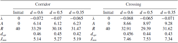
5. Conclusion and outlook
We extended the anisotropic interaction model proposed in [Reference Totzeck34] by including body size and thus additional volume exclusion effects. Numerical studies indicate that body size has an influence on the lane formation process. In fact, it seems that a smaller body size leads to a higher number of lanes formed and vice versa. Moreover, we investigated the fundamental diagram of the dynamics and found that higher densities lead to lower velocities. This observation was expected from other experiments and underlines the feasibility of the approach.
Due to the ODE formulation of the model, we were able to analyze the model in terms of well-posedness and further rigorously derive a gradient-based descent algorithm for a calibration problem using real data. The optimal scaling parameters for the collision avoidance and the repulsion strength turn out to match very well for the two tested scenarios. For the attraction parameter, we find different values for the two scenarios. We suspect that this is related to the post-collision behavior of the model.
To prove or discard this conjecture is interesting future work. Moreover, the rigorous analysis of stationary states like the lanes in the corridor case and the traveling waves in the crossing case is planned for future investigations.
Acknowledgement
ZT acknowledges funding by the German Academic Exchange Service programme “Mathematics in Industry and Commerce, MIC”.
Competing interests
The authors hereby declare that there are no competing interests.
Appendix A. Boundedness of
$\nabla M(\cdot )$

We show the boundedness of $\nabla M(v_i, v_j )$
, where
$\nabla M(v_i, v_j )$
, where
 \begin{equation*} \nabla M(v_i, v_j ) = \left (\frac {dM(v_i, v_j )}{d {v}_i}, \frac {dM(v_i, v_j )}{d {v}_j}\right ), \end{equation*}
with
 \begin{equation*} \frac {dM}{d {v}_i}= \begin {pmatrix} -\sin \alpha & -\cos \alpha \\ \cos \alpha & -\sin \alpha \end {pmatrix} \cdot \frac {d\alpha }{d {v}_i}, \end{equation*}
 \begin{equation} \frac{d\alpha }{d{v}_i} = \begin{cases} -\lambda \frac{1}{ \sqrt{(\left \lVert{v_i} \right \rVert \left \lVert{v_j} \right \rVert ) ^2 - \langle{v_i},{v_j} \rangle ^2}}\left ({v_j} - \langle{v_i},{v_j} \rangle \frac{{v_i}}{\left \lVert{v_i}\right \rVert ^2}\right ), & \text{if }{v_i},{v_j}\neq 0 \\[5pt] 0, & \text{else} \end{cases}. \end{equation}
We, therefore, transform the system to polar coordinates and introduce the notations $v_i ={\begin{pmatrix} r_1 \cos \phi _1 \\[4pt] r_1 \sin \phi _1 \end{pmatrix}, }$
and
$v_i ={\begin{pmatrix} r_1 \cos \phi _1 \\[4pt] r_1 \sin \phi _1 \end{pmatrix}, }$
and $v_j ={\begin{pmatrix} r_2 \cos \phi _2 \\[4pt] r_2 \sin \phi _2 \end{pmatrix} }$
. Here,
$v_j ={\begin{pmatrix} r_2 \cos \phi _2 \\[4pt] r_2 \sin \phi _2 \end{pmatrix} }$
. Here, $r_1$
and
$r_1$
and $r_2$
are positive scalars. It is clear that
$r_2$
are positive scalars. It is clear that $\left |{\begin{pmatrix} -\sin \alpha & -\cos \alpha \\[4pt] \cos \alpha & -\sin \alpha \end{pmatrix} }\right | \lt \infty$
. Then, we need to show
$\left |{\begin{pmatrix} -\sin \alpha & -\cos \alpha \\[4pt] \cos \alpha & -\sin \alpha \end{pmatrix} }\right | \lt \infty$
. Then, we need to show $\left | \frac{d\alpha }{d{v}_i} \right | = C\lt \infty$
.
$\left | \frac{d\alpha }{d{v}_i} \right | = C\lt \infty$
.
For further usage, we define
 \begin{equation*}{\left \lVert v_i\right \rVert _2 = r_1},\quad {\left \lVert v_j\right \rVert _2 = r_2} \text { and } { \langle {v_i}, {v_j} \rangle } = r_1 r_2 (\cos \phi _1 \cos \phi _2 + \sin \phi _1 \sin \phi _2). \end{equation*}
Substituting the velocity vectors in (A1), we get
 \begin{align*}{\left |\frac{d\alpha }{d{v}_i} \right |}_2 &= \left | \frac{-\lambda }{ \sqrt{r_1^2 r_2^2 - (r_1 r_2\cos (\phi _1 - \phi _2) )^2 }} \right |{\left | \begin{pmatrix} r_2 \cos \phi _2 \\[4pt] r_2 \sin \phi _2 \end{pmatrix} - r_1 r_2\cos (\phi _1 - \phi _2) \frac{1}{r_1^2} \begin{pmatrix} r_1 \cos \phi _1 \\[4pt] r_1 \sin \phi _1 \end{pmatrix} \right |}_2 \\[4pt] & = \frac{\left | \lambda \right | }{ r_1 r_2 \left |\sin (\phi _1 - \phi _2) \right | }{\left | \begin{pmatrix} r_2 \cos \phi _2 - r_2 \cos \phi _1 \cos (\phi _1 - \phi _2) \\[4pt] r_2 \sin \phi _2 - r_2 \sin \phi _1 \cos (\phi _1 - \phi _2) \end{pmatrix} \right |}_2\\[4pt] & = \frac{\left | \lambda \right | }{ r_1 r_2 \left |\sin (\phi _1 - \phi _2) \right | } \left [r_2^2{(\cos \phi _2 - \cos \phi _1 \cos (\phi _1 - \phi _2))}^2 \right .\\[4pt] &\left .+ r_2^2{( \sin \phi _2 - \sin \phi _1 \cos (\phi _1 - \phi _2) )}^2\right ]^{\frac{1}{2}} \\[4pt] &= \frac{\left | \lambda \right | }{ r_1 r_2 \left |\sin (\phi _1 - \phi _2) \right | } r_2 \sqrt{1 - \cos ^2 (\phi _1 - \phi _2)} = \frac{\left | \lambda \right | }{ r_1 } \lt \infty. \end{align*}
Analogously, we can show that $\left |\frac{d\alpha }{d{v}_j} \right |_2 =\frac{\left | \lambda \right | }{ r_2 }\lt \infty$
. This proves the boundedness of
$\left |\frac{d\alpha }{d{v}_j} \right |_2 =\frac{\left | \lambda \right | }{ r_2 }\lt \infty$
. This proves the boundedness of $\nabla M(v_i, v_j )$
as desired.
$\nabla M(v_i, v_j )$
as desired.
Appendix B. Tensor
$d_{v_i}M^*(v_i,v_j)$

Here, we present the details of the mathematical manipulations made to tensor $d_{v_i}M(v_i,v_j)$
in the derivation of
$d_{v_i}M(v_i,v_j)$
in the derivation of $d_{v_i}M^*(v_i,v_j)$
. Note that
$d_{v_i}M^*(v_i,v_j)$
. Note that $d_{v_i}M(v_i,v_j)$
is a tensor with dimension
$d_{v_i}M(v_i,v_j)$
is a tensor with dimension $2\times 2 \times 2$
given by:
$2\times 2 \times 2$
given by:
 \begin{align} d_{v_i}M\left ( v_{i}, v_{j}\right ) = \begin{pmatrix} -\sin \alpha _{ij} \cdot d_{v_i}\alpha _{ij} & -\cos \alpha _{ij} \cdot d_{v_i}\alpha _{ij}\\[5pt] \cos \alpha _{ij} \cdot d_{v_i}\alpha _{ij} & -\sin \alpha _{ij} \cdot d_{v_i}\alpha _{ij} \end{pmatrix}_{2\times 2 \times 2}, \end{align}
where
 \begin{align*} d_{ v_i} \alpha _{ij} = \begin{cases} -\lambda \cdot \frac{1}{ \sqrt{(\left \lVert v_i\right \rVert \left \lVert v_j\right \rVert )^2-\langle v_i, v_j \rangle ^2 }} \cdot \left ( v_j - \langle v_i, v_j \rangle \frac{v_i}{\left \lVert v_i\right \rVert ^2} \right ), & \text{for } v_i \neq 0, \ v_j \neq 0, \\[5pt] \vec{0}, & \text{else} \end{cases}. \end{align*}
The elements of the tensor $d_{v_i}M\left ( v_{i}, v_{j}\right )$
in (B1) are denoted as:
$d_{v_i}M\left ( v_{i}, v_{j}\right )$
in (B1) are denoted as:
 \begin{equation*} d_{v_i}M(v_i,v_j) = \begin {pmatrix} \begin {pmatrix} m_{11} \\[4pt] m_{12} \end {pmatrix} & \begin {pmatrix} m_{21} \\[4pt] m_{22} \end {pmatrix} \\[15pt] \begin {pmatrix} m_{31} \\[4pt] m_{32} \end {pmatrix} & \begin {pmatrix} m_{41} \\[4pt] m_{42} \end {pmatrix} \end {pmatrix}, \quad \text {with} \quad { m_{ij} \in {\mathbb {R}}, i=1,\dots,4, j=1,2, } \end{equation*}
then its dual $d_{v_i}M^*(v_i,v_j)$
in (3.6) is the transposed tensor after swapping its axes, as given below:
$d_{v_i}M^*(v_i,v_j)$
in (3.6) is the transposed tensor after swapping its axes, as given below:
 \begin{equation*} d_{v_i}M^*(v_i,v_j) = \begin {pmatrix} \begin {pmatrix} m_{11} \\[4pt] m_{21} \end {pmatrix} & \begin {pmatrix} m_{31} \\[4pt] m_{41} \end {pmatrix} \\[15pt] \begin {pmatrix} m_{12} \\[4pt] m_{22} \end {pmatrix} & \begin {pmatrix} m_{32} \\[4pt] m_{42} \end {pmatrix} \end {pmatrix}. \end{equation*}
Appendix C. Existence of adjoint states
For completeness, we give the assumptions and the statement of Corollary 1.3 of [Reference Hinze, Pinnau, Ulbrich and Ulbrich21] which we use to prove the existence of adjoint states in Section 3.2.2.
Assumption 3. Let the following assumptions hold:
-
(A1)
$U_{\text{ad}} \subset U$
is nonempty, convex, and closed.
-
(A2)
$J \colon Y \times U \rightarrow{\mathbb{R}}$
and
$e \colon Y \times U \rightarrow Z$
are continuously Freéchet differentiable and
$U,Y,Z$
are Banach spaces.
-
(A3) For all
$u \in V$
in a neighbourhood
$V \subset U$
of U ad, the state equation
$e(y,u) = 0$
has a unique solution
$y = y(u) \in Y$
. -
(A4)
$e_y(y(u),u) \in \mathcal L(Y,Z)$
has a bounded inverse for all
$u \in V.$


Proposition 1 (Existence of adjoint states [Reference Hinze, Pinnau, Ulbrich and Ulbrich21]). Let $(\bar y, \bar u)$
be an optimal solution of
$(\bar y, \bar u)$
be an optimal solution of
 \begin{equation*}\min J(y,u) \text { subject to } e(y,u)=0\end{equation*}
and let Assumption 3 hold.
Then there exists an adjoint state (or Lagrange multiplier) $\bar p \in Z^*$
such that the following optimality conditions hold
$\bar p \in Z^*$
such that the following optimality conditions hold
 \begin{align*} &\langle e(\bar y,\bar u), p \rangle _{Z,Z^*} = 0 &&\forall p \in Z^*, \\ &\langle L_y(\bar y, \bar u, \bar p), v \rangle _{Y^*,Y} = 0 &&\forall v \in Y^*, \\ &\bar u \in U_{\text{ad}}, \langle L_u(\bar y, \bar u, \bar p), u-\bar u \rangle _{U^*,U} \ge 0, &&\forall u\in U_{\text{ad}}. \end{align*}


 Open access