


1 Introduction
Higher dimensional, physically relevant, dynamical systems often possess features that can be studied using techniques from one-dimensional dynamical systems. Indeed, often a one-dimensional discrete dynamical system captures essential features of a higher dimensional flow. For example, for the Lorenz flow [Reference Lorenz22], one may study the return mapping to a plane transverse to its stable manifold, the stable manifold intersects the plane in a curve, and the return mapping to this curve is a (discontinuous) one-dimensional dynamical system known as a Lorenz mapping, see paper [Reference Tucker47]. This approach has been very fruitful in the study of the Lorenz flow. It would be difficult to cite all the papers studying this famous dynamical system, but for example see papers [Reference Afraĭmovič, Bykov and Shil’nikov1, Reference Arneodo, Coullet and Tresser3, Reference Gambaudo, Procaccia, Thomae and Tresser15, Reference Guckenheimer and Williams18, Reference Rovella39, Reference Williams49]. The success of the use of the one-dimensional Lorenz mapping in studying the flow has led to an extensive study of these interval mappings, see papers [Reference Brandão6, Reference Gaidashev and Winckler14, Reference Keller, St. Pierre and Fiedler19, Reference Labarca and Moreira20, Reference Martens and de Melo26, Reference Martens and Winckler29, Reference Martens and Winckler30, Reference St. Pierre43, Reference Winckler50] among many others. Great progress in understanding the Cherry flow on a two-torus has followed from a similar approach [Reference Aranson, Zhuzhoma and Medvedev2, Reference Cherry8, Reference de Melo11, Reference Martens, van Strien, de Melo and Mendes28, Reference Mendes33–Reference Palmisano38, Reference Saghin and Vargas40].
In this paper, we study a class of Lorenz mappings, which have ‘gaps’ in their ranges. These mappings arise as return mappings for the Lorenz flow and for certain Cherry flows. They are also among the first examples of mappings with a wandering interval – the gap. This phenomenon is ruled out for
 $\mathcal C^{1+\mathrm {Zygmund}}$
mappings with a non-flat critical point by van Strien and Vargas [Reference van Strien and Vargas48]. In fact, Berry and Mestel [Reference Berry and Mestel5] proved that Lorenz mappings satisfying a certain bounded nonlinearity condition have a wandering interval if and only if they have a renormalization which is a gap mapping. See the introduction of paper [Reference Gouveia and Colli17] for a detailed history of gap mappings.
$\mathcal C^{1+\mathrm {Zygmund}}$
mappings with a non-flat critical point by van Strien and Vargas [Reference van Strien and Vargas48]. In fact, Berry and Mestel [Reference Berry and Mestel5] proved that Lorenz mappings satisfying a certain bounded nonlinearity condition have a wandering interval if and only if they have a renormalization which is a gap mapping. See the introduction of paper [Reference Gouveia and Colli17] for a detailed history of gap mappings.
The main result of this paper concerns the structure of the topological conjugacy classes of
 $\mathcal C^4$
dissipative gap mappings. Roughly, these are discontinuous mappings with two orientation preserving branches, whose derivatives are bounded between zero and one. They are defined in Definition 2.1.
$\mathcal C^4$
dissipative gap mappings. Roughly, these are discontinuous mappings with two orientation preserving branches, whose derivatives are bounded between zero and one. They are defined in Definition 2.1.
Theorem 1.1. The topological conjugacy class of an infinitely renormalizable
 $\mathcal C^4$
dissipative gap mapping is a
$\mathcal C^4$
dissipative gap mapping is a
 $\mathcal C^1$
-manifold of codimension-one in the space of dissipative gap maps.
$\mathcal C^1$
-manifold of codimension-one in the space of dissipative gap maps.
To obtain this result, we prove the hyperbolicity of renormalization for dissipative gap mappings. In the usual approach to renormalization, one considers renormalization as a restriction of a high iterate of a mapping. While this is conceptually straightforward, it is technically challenging as the composition operator acting on the space of, say,
 $\mathcal {C}^4$
functions is not differentiable. Nevertheless, we are able to show that the tangent space admits a hyperbolic splitting. To do this, we work in the decomposition space introduced by Martens in [Reference Martens25], see §3 for the necessary background.
$\mathcal {C}^4$
functions is not differentiable. Nevertheless, we are able to show that the tangent space admits a hyperbolic splitting. To do this, we work in the decomposition space introduced by Martens in [Reference Martens25], see §3 for the necessary background.
Theorem 1.2. The renormalization operator
 ${\mathcal R}$
acting on the space of dissipative gap mappings has a hyperbolic splitting. More precisely, if f is an infinitely renormalizable
${\mathcal R}$
acting on the space of dissipative gap mappings has a hyperbolic splitting. More precisely, if f is an infinitely renormalizable
 ${\mathcal C}^3$
dissipative gap mapping then for any
${\mathcal C}^3$
dissipative gap mapping then for any
 $\delta \in (0,1),$
and for all n sufficiently big, the derivative of the renormalization operator acting on the decomposition space
$\delta \in (0,1),$
and for all n sufficiently big, the derivative of the renormalization operator acting on the decomposition space
 $\underline {\mathcal {D}}$
satisfies the following.
$\underline {\mathcal {D}}$
satisfies the following.
-
•
 $T_{\underline {\mathcal {R}}_{\underline {\mathcal {R}}^n\underline f}} \underline {\mathcal {D}}=E^u\oplus E^s,$
and the subspace
$E^u$
is one-dimensional.
$T_{\underline {\mathcal {R}}_{\underline {\mathcal {R}}^n\underline f}} \underline {\mathcal {D}}=E^u\oplus E^s,$
and the subspace
$E^u$
is one-dimensional. -
• For any vector
$v\in E^u$
, we have that
$\|D\underline {\mathcal {R}}_{\underline {\mathcal {R}}^n\underline f}v\|\geq \unicode{x3bb} _1\|v\|$
, where
$|\unicode{x3bb} _1|>1/\delta $
. -
• For any
$v\in E^s$
, we have that
$\|D\underline {\mathcal {R}}_{\underline {\mathcal {R}}^n\underline f}v\|\leq \unicode{x3bb} \|v\|$
, where
$|\unicode{x3bb} |<\delta $
.


Gap mappings can be regarded as discontinuous circle mappings, and indeed they have a well-defined rotation number [Reference Brette7], and they are infinitely renormalizable precisely when the rotation number is irrational. Consequently, from a combinatorial point of view they are similar to critical circle mappings. However, unlike critical circle mappings, the geometry of gap mappings is unbounded. For example, for critical circle mappings the quotient of the lengths of successive renormalization intervals is bounded away from zero and infinity [Reference de Faria and de Melo9], but for gap mappings it diverges very fast [Reference Gouveia and Colli17]. As a result, the renormalization operator for gap mappings does not seem to possess a natural extension to the limits of renormalization (cf. [Reference Martens and Palmisano27]).
Renormalization theory was introduced into dynamical systems from statistical physics by Feigenbaum [Reference Feigenbaum13], and Tresser and Coullet [Reference Tresser and Coullet45, Reference Tresser and Coullet46] in the 1970s to explain the universality phenomena they observed in the quadratic family. They conjectured that the period-doubling renormalization operator acting on an appropriate space of analytic unimodal mappings is hyperbolic. The first proof of this conjecture was obtained using computer assistance by Lanford [Reference Lanford21]. The conjecture can be extended to all combinatorial types and to multimodal mappings. A conceptual proof was given for analytic unimodal mappings of any combinatorial type in the works of Sullivan [Reference Sullivan44] (see also [Reference de Melo and van Strien12]), McMullen [Reference McMullen31, Reference McMullen32], Lyubich [Reference Lyubich23, Reference Lyubich24], and Avila and Lyubich [Reference Avila and Lyubich4]. This was extended to certain smooth mappings by de Faria, de Melo and Pinto [Reference de Faria, de Melo and Pinto10], and to analytic mappings with several critical points and bounded combinatorics by Smania [Reference Smania41, Reference Smania42]. Renormalization is intimately related with rigidity theory, and in many contexts, e.g. interval mappings and critical circle mappings, exponential convergence of renormalization implies that two topologically conjugate infinitely renormalizable mappings are smoothly conjugate on their (measure-theoretic) attractors. However, for gap mappings, it is not the case that exponential convergence of renormalization implies rigidity; indeed, in general, one can not expect topologically conjugate gap mappings to be
 $\mathcal C^1$
conjugate [Reference Gouveia and Colli17].
$\mathcal C^1$
conjugate [Reference Gouveia and Colli17].
The aforementioned results on renormalization of interval mappings all depend on complex analytic tools and, consequently, many of the tools developed in these works can only be applied to mappings with a critical point of integer order. The goal of studying mappings with arbitrary critical order was one of Martens’ motivations for introducing the decomposition space, mentioned above. This purely real approach has led to results on the renormalization in various contexts. Martens [Reference Martens25] used this approach to establish the existence of periodic points of renormalization of any combinatorial type for unimodal mappings
 $x\mapsto x^\alpha +c$
, where
$x\mapsto x^\alpha +c$
, where
 $\alpha>1$
is not necessarily an integer. For Lorenz mappings of certain monotone combinatorial types, Martens and Winckler [Reference Martens and Winckler29] proved that there exists a global two-dimensional strong unstable manifold at every point in the limit set of renormalization using this approach. Martens and Palmisano [Reference Martens and Palmisano27] studied renormalization acting on the decomposition space for infinitely renormalizable critical circle mappings with a flat interval. They proved that for certain mappings with stationary, Fibonacci, combinatorics that the renormalization operator is hyperbolic, and that the class of mappings with Fibonacci combinatorics is a
$\alpha>1$
is not necessarily an integer. For Lorenz mappings of certain monotone combinatorial types, Martens and Winckler [Reference Martens and Winckler29] proved that there exists a global two-dimensional strong unstable manifold at every point in the limit set of renormalization using this approach. Martens and Palmisano [Reference Martens and Palmisano27] studied renormalization acting on the decomposition space for infinitely renormalizable critical circle mappings with a flat interval. They proved that for certain mappings with stationary, Fibonacci, combinatorics that the renormalization operator is hyperbolic, and that the class of mappings with Fibonacci combinatorics is a
 $\mathcal C^1$
manifold.
$\mathcal C^1$
manifold.
Analytic gap mappings were studied by Gouveia and Colli [Reference Gouveia and Colli16, Reference Gouveia and Colli17] using different methods to those that we use here. In the former paper, they proved hyperbolicity of renormalization in the special case of affine dissipative gap mappings, and in the latter paper, they proved that the topological conjugacy classes of analytic infinitely renormalizable dissipative gap mappings are analytic manifolds. We appropriately generalize these two results to the
 $\mathcal C^4$
case. Since the renormalization operator does not extend to the limits of renormalization, it seems to be difficult to build on the hyperbolicity result for affine mappings to extend it to smooth mappings (similar to what was done in paper [Reference de Faria, de Melo and Pinto10]), and so we follow a different approach. Gouveia and Colli [Reference Gouveia and Colli17] also proved that two topologically conjugate dissipative gap mappings are Hölder conjugate. We improve this rigidity result, and give a simple proof that topologically conjugate dissipative gap mappings are quasisymmetrically conjugate, see Proposition 2.8.
$\mathcal C^4$
case. Since the renormalization operator does not extend to the limits of renormalization, it seems to be difficult to build on the hyperbolicity result for affine mappings to extend it to smooth mappings (similar to what was done in paper [Reference de Faria, de Melo and Pinto10]), and so we follow a different approach. Gouveia and Colli [Reference Gouveia and Colli17] also proved that two topologically conjugate dissipative gap mappings are Hölder conjugate. We improve this rigidity result, and give a simple proof that topologically conjugate dissipative gap mappings are quasisymmetrically conjugate, see Proposition 2.8.
This paper is organized as follows: in §2, we will provide the necessary background material on gap mappings, and in §3, we will describe the decomposition space of infinitely renormalizable gap mappings. The estimate of the derivative of renormalization operator is done in §4, and it is the key technical result of our work. In our setting, we are able to obtain fairly complete results without any restrictions on the combinatorics of the mappings. In §5, we use the estimates of §4 and ideas from paper [Reference Martens and Palmisano27] to show that the renormalization operator is hyperbolic and that the conjugacy classes of dissipative gap mappings are
 $\mathcal C^1$
manifolds.
$\mathcal C^1$
manifolds.
2 Preliminaries
2.1 The dynamics of gap maps
In this section, we collect the necessary background material on gap mappings, see paper [Reference Gouveia and Colli17] for further results.
A Lorenz map is a function
 $f:[a_L, a_R] \setminus \{ 0 \} \rightarrow [a_L, a_R]$
satisfying:
$f:[a_L, a_R] \setminus \{ 0 \} \rightarrow [a_L, a_R]$
satisfying:
-
(i)
$a_L< 0 < a_R$
; -
(ii) f is continuous and strictly increasing in the intervals
$[a_L,0)$
and
$(0,a_R]$
; -
(iii) the left and right limits at
$0$
are
$f(0^-)=a_R$
and
$f(0^+)=a_L$
.


A gap map is a Lorenz map f that is not surjective, that is, a map satisfying conditions (i), (ii), (iii) with
 $f(a_L)> f(a_R)$
. In this case the gap is the interval
$f(a_L)> f(a_R)$
. In this case the gap is the interval
 $G_f=(f(a_R), f(a_L))$
. When it will not cause confusion, we omit the subscript and denote the gap by G.
$G_f=(f(a_R), f(a_L))$
. When it will not cause confusion, we omit the subscript and denote the gap by G.
Definition 2.1. A dissipative gap map is a gap map f that is differentiable in
 $[a_L, a_R] \setminus \{ 0 \}$
and satisfies:
$[a_L, a_R] \setminus \{ 0 \}$
and satisfies:
 $0 < f'(x) \leq \nu $
for every
$0 < f'(x) \leq \nu $
for every
 $x \in [a_L, a_R] \setminus \{ 0 \}$
, and for some real number
$x \in [a_L, a_R] \setminus \{ 0 \}$
, and for some real number
 $\nu = \nu _f \in (0,1)$
.
$\nu = \nu _f \in (0,1)$
.
Each dissipative gap mapping is determined by a mapping to the left of the discontinuity, a mapping to the right of the discontinuity and the relative position of the discontinuity in the interval. Hence it is convenient to describe the space of dissipative gap mappings as follows: Consider
 $$ \begin{align} \mathcal{D}_L^k &= \{ u_L:[-1,0) \rightarrow \mathbb{R}; \; u_L\in\mathrm{Diff}_+^k[-1,0], u_L(0^-)=0, \nonumber\\ &\,\quad \; \text{and} \; \text{there exists}\ \nu \in (0,1) \; \text{such that} \; 0 < u_L'(x) \leq \nu, \; \text{for all}\ \ x \in [-1,0) \}, \end{align} $$
 $$ \begin{align} \mathcal{D}_R^k &= \{ u_R:(0, +1] \rightarrow \mathbb{R}; \; u_R \in\mathrm{Diff}_+^k[0,1], u_R(0^+)=0, \nonumber\\ &\,\quad \; \text{and} \; \text{there exists}\ \nu \in (0,1) \; \text{such that} \; 0 < u_R'(x) \leq \nu, \; \text{for all}\ \ x \in [0,1) \}, \end{align} $$
and
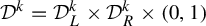 $\mathcal {D}^k = \mathcal {D}_L^k \times \mathcal {D}_R^k \times (0,1)$
, where
$\mathcal {D}^k = \mathcal {D}_L^k \times \mathcal {D}_R^k \times (0,1)$
, where
 $\mathrm {Diff}_+^k[x,y]$
denotes the space of orientation preserving
$\mathrm {Diff}_+^k[x,y]$
denotes the space of orientation preserving
 $\mathcal C^k$
diffeomorphisms on
$\mathcal C^k$
diffeomorphisms on
 $(x,y)$
, which are continuous on
$(x,y)$
, which are continuous on
 $[x,y]$
. We will always assume that
$[x,y]$
. We will always assume that
 $k\geq 3,$
and unless otherwise stated, the reader can assume that
$k\geq 3,$
and unless otherwise stated, the reader can assume that
 $k=3.$
For each element
 $(u_L, u_R, b) \in \mathcal {D}^k$
, we associate a function
$(u_L, u_R, b) \in \mathcal {D}^k$
, we associate a function
 $f:[-1,1] \setminus \{ 0 \} \rightarrow [-1,1]$
defined by
$f:[-1,1] \setminus \{ 0 \} \rightarrow [-1,1]$
defined by
 $$ \begin{align} f(x) = \left\{ \begin{array}{@{}ll} u_L(x)+b, & x \in [-1,0), \\[3pt] u_R(x)+b-1, & x \in (0,+1], \end{array}\right. \end{align} $$
and take
 $\nu = \nu _f \in (0,1)$
that bounds the derivative on each branch from above. It is not difficult to check that the interval
$\nu = \nu _f \in (0,1)$
that bounds the derivative on each branch from above. It is not difficult to check that the interval
 $[b-1,b]$
is invariant under f, and f restricted to
$[b-1,b]$
is invariant under f, and f restricted to
 $[b-1, b] \setminus \{ 0 \}$
is a dissipative gap map. Observe that the parameter b determines the position of the discontinuity in the interval. For the sake of simplicity, we write
$[b-1, b] \setminus \{ 0 \}$
is a dissipative gap map. Observe that the parameter b determines the position of the discontinuity in the interval. For the sake of simplicity, we write
 $f=(u_L, u_R, b)$
, and we use the following notation for the left and right branches of f:
$f=(u_L, u_R, b)$
, and we use the following notation for the left and right branches of f:
 $$ \begin{align} \begin{array}{@{}ll} f_L(x) = u_L(x)+b, & x <0,\\ f_R(x) = u_R(x)+b-1, & x>0, \end{array} \end{align} $$
We endow
 $\mathcal {D}^k = \mathcal {D}_L^k \times \mathcal {D}_R^k \times (0,1)$
with the product topology. It is important to note that a gap map g defined in an interval
$\mathcal {D}^k = \mathcal {D}_L^k \times \mathcal {D}_R^k \times (0,1)$
with the product topology. It is important to note that a gap map g defined in an interval
 $[a_L, a_R]$
can be rescaled by a linear conjugacy in such a way as to be defined in
$[a_L, a_R]$
can be rescaled by a linear conjugacy in such a way as to be defined in
 $[b-1,b]$
. After rescaling and extending g, we obtain a function f defined in
$[b-1,b]$
. After rescaling and extending g, we obtain a function f defined in
 $[-1,1] \setminus \{0\}$
which is a triple
$[-1,1] \setminus \{0\}$
which is a triple
 $f=(f_L, f_R, b)$
in
$f=(f_L, f_R, b)$
in
 $\mathcal D^k.$
Since
$\mathcal D^k.$
Since
 $[b-1,b]$
is a trapping region for f, it will be enough to work with the restriction of f to
$[b-1,b]$
is a trapping region for f, it will be enough to work with the restriction of f to
 $[b-1,b] \setminus \{0\}$
and it is not important how f is extended. Thus we set
$[b-1,b] \setminus \{0\}$
and it is not important how f is extended. Thus we set
 $a_L = b-1$
and
$a_L = b-1$
and
 $a_R=b.$
For more details, see §1.2 of paper [Reference Gouveia and Colli17].
$a_R=b.$
For more details, see §1.2 of paper [Reference Gouveia and Colli17].
Definition 2.2. Let
 $f:[b-1, b] \setminus \{0 \} \rightarrow [b-1, b]$
be a dissipative gap map. We define the sign of f by
$f:[b-1, b] \setminus \{0 \} \rightarrow [b-1, b]$
be a dissipative gap map. We define the sign of f by
 $$ \begin{align} \sigma_f:= \left\{ \begin{array}{@{}ll} - & \text{ if } b \leq 1/2,\\ + & \text{ if } b> 1/2. \end{array} \right. \end{align} $$
It is an easy consequence of this definition that for a dissipative gap map f, we have
 $\sigma _f=-$
if
$\sigma _f=-$
if
 $G \subset [b-1,0)$
and
$G \subset [b-1,0)$
and
 $\sigma _f=+$
when
$\sigma _f=+$
when
 $G \subset (0,b]$
.
$G \subset (0,b]$
.
2.2 Renormalization of dissipative gap mappings
Definition 2.3. A dissipative gap map
 $f:[b-1, b] \setminus \{0 \} \rightarrow [b-1, b]$
is renormalizable if there exists a positive integer k such that:
$f:[b-1, b] \setminus \{0 \} \rightarrow [b-1, b]$
is renormalizable if there exists a positive integer k such that:
-
(a)
$0 \notin \bigcup _{i=0}^k \overline {f^i(G)}$
; -
(b) either
-
–
$\overline {G}, \overline {f(G)}, \ldots , \overline {f^{k-1}(G)} \subset (b-1,0)$
and
$\overline {f^k(G)} \subset (0,b)$
or -
–
$\overline {G}, \overline {f(G)}, \ldots , \overline {f^{k-1}(G)} \subset (0,b)$
and
$\overline {f^k(G)} \subset (b-1,0).$
-


Remark 2.4. The positive number k in Definition 2.3 is chosen to be minimal so that (a) and (b) hold.
By [Reference Gouveia and Colli17, Proposition 2.8], and the mean value theorem, the renormalization of a dissipative gap map is again a dissipative gap map.
Definition 2.5. Let
 $f:[b-1, b] \setminus \{0 \} \rightarrow [b-1, b]$
be a renormalizable dissipative gap map, and consider
$f:[b-1, b] \setminus \{0 \} \rightarrow [b-1, b]$
be a renormalizable dissipative gap map, and consider
 $I'= [a_L', a_R' ]=I_f'$
the interval containing
$I'= [a_L', a_R' ]=I_f'$
the interval containing
 $0$
whose boundary points are the boundary points of
$0$
whose boundary points are the boundary points of
 $f^{k-1}(G)$
and
$f^{k-1}(G)$
and
 $f^k(G)$
which are nearest to
$f^k(G)$
which are nearest to
 $0$
, that is
$0$
, that is
 $$ \begin{align} \begin{array}{@{}cl} I'= [f^k(b-1), f^{k+1}(b)] & \text{ for } \sigma_f = -,\\ I'= [f^{k+1}(b-1), f^k(b)] & \text{ for } \sigma_f=+. \end{array} \end{align} $$
The first return map
 $R=R_f$
to
$R=R_f$
to
 $I'$
is given by
$I'$
is given by
 $$ \begin{align} R(x)= \left\{ \begin{array}{@{}ll} f^{k+2}(x) & \text{ if } x \in [f^k(b-1),0),\\ f^{k+1}(x) & \text{ if } x \in (0,f^{k+1}(b)], \end{array}\right. \end{align} $$
in the case where
 $\sigma _f=-$
, and
$\sigma _f=-$
, and
 $$ \begin{align} R(x)= \left\{ \begin{array}{@{}ll} f^{k+1}(x) & \text{ if } x \in [f^{k+1}(b-1),0),\\ f^{k+2}(x) & \text{ if } x \in (0,f^{k}(b)], \end{array}\right. \end{align} $$
in the case where
 $\sigma _f=+$
. The renormalization of f,
$\sigma _f=+$
. The renormalization of f,
 $\mathcal {R}f$
, is the first return map R rescaled and normalized to the interval
$\mathcal {R}f$
, is the first return map R rescaled and normalized to the interval
 $[-1,1]$
and given by
$[-1,1]$
and given by
 $$ \begin{align} \mathcal{R}f(x)= \frac{1}{|I'|}R(|I'|x) \end{align} $$
for every
 $x \in [-1,1] \setminus \{0 \}$
.
$x \in [-1,1] \setminus \{0 \}$
.
In terms of the branches
 $f_L$
and
$f_L$
and
 $f_R$
defined in (2.4), the first return map R is given by
$f_R$
defined in (2.4), the first return map R is given by
 $$ \begin{align} R(x)= \left\{ \begin{array}{@{}ll} f_L^k {{\kern0.5pt}\circ{\kern0.5pt}} f_R {{\kern0.5pt}\circ{\kern0.5pt}} f_L (x) & \text{ if } x \in [f^k(b-1),0),\\ [4pt] f_L^k {{\kern0.5pt}\circ{\kern0.5pt}} f_R (x) & \text{ if } x \in (0,f^{k+1}(b)], \end{array}\right. \end{align} $$
in the case where
 $\sigma _f=-$
, and
$\sigma _f=-$
, and
 $$ \begin{align} R(x)= \left\{ \begin{array}{@{}ll} f_R^k {{\kern0.5pt}\circ{\kern0.5pt}} f_L (x) & \text{ if } x \in [f^{k+1}(b-1),0),\\ [4pt] f_R^k {{\kern0.5pt}\circ{\kern0.5pt}} f_L {{\kern0.5pt}\circ{\kern0.5pt}} f_R (x) & \text{ if } x \in (0,f^{k}(b)], \end{array}\right. \end{align} $$
in the case where
 $ \sigma _f=+ $
.
$ \sigma _f=+ $
.
From Definition 2.5, we have a natural operator which sends a renormalizable dissipative gap map f to its renormalization
 $\mathcal {R}f$
, which is also a dissipative gap map.
$\mathcal {R}f$
, which is also a dissipative gap map.
Definition 2.6. The renormalization operator is defined by
 $$ \begin{align} \begin{array}{l@{}lll} \mathcal{R} \! :\! &\mathcal{D}_{\mathcal{R}}^k & \rightarrow & \mathcal{D}^k \\ & f & \mapsto & \mathcal{R}f \end{array} \end{align} $$
where
 $\mathcal {R}f(x)= ({1}/{|I'|})R(|I'|x)$
, and
$\mathcal {R}f(x)= ({1}/{|I'|})R(|I'|x)$
, and
 $\mathcal {D}_{\mathcal {R}}^k \subset \mathcal {D}^k$
is the subset of all renormalizable dissipative gap maps in
$\mathcal {D}_{\mathcal {R}}^k \subset \mathcal {D}^k$
is the subset of all renormalizable dissipative gap maps in
 $\mathcal {D}^k$
.
$\mathcal {D}^k$
.
Although a dissipative gap map is not defined at
 $0$
, we define the lateral orbits of
$0$
, we define the lateral orbits of
 $0$
taking
$0$
taking
 $0_j^+ = f^j(0^+)= \lim _{x \rightarrow 0^+}f^j(x)$
and
$0_j^+ = f^j(0^+)= \lim _{x \rightarrow 0^+}f^j(x)$
and
 $0_j^- = f^j(0^-)= \lim _{x \rightarrow 0^-}f^j(x)$
. We first observe that
$0_j^- = f^j(0^-)= \lim _{x \rightarrow 0^-}f^j(x)$
. We first observe that
 $0_j^+=f^{j-1}(b-1)$
and
$0_j^+=f^{j-1}(b-1)$
and
 $0_j^-=f^{j-1}(b)$
. The left and right future orbits of
$0_j^-=f^{j-1}(b)$
. The left and right future orbits of
 $0$
are the sequences
$0$
are the sequences
 $(0_j^+)_{j \geq 1}$
and
$(0_j^+)_{j \geq 1}$
and
 $(0_j^-)_{j \geq 1}$
, which are always defined unless there exists
$(0_j^-)_{j \geq 1}$
, which are always defined unless there exists
 $j \geq 1$
such that either
$j \geq 1$
such that either
 $0_j^+ = 0$
or
$0_j^+ = 0$
or
 $0_j^-=0$
. Using this notation for the interval
$0_j^-=0$
. Using this notation for the interval
 $I'$
defined in (2.6), we obtain
$I'$
defined in (2.6), we obtain
 $$ \begin{align} I'=\left\{ \begin{array}{@{}ll} [0_{k+1}^+,0_{k+2}^-] = [f_L^k (b-1),f_L^k {{\kern0.5pt}\circ{\kern0.5pt}} f_R(b)] &\text{ for } \sigma_f = -, \\ [4pt] [0_{k+2}^+,0_{k+1}^-] = [f_R^k {{\kern0.5pt}\circ{\kern0.5pt}} f_L(b-1),f_R^k (b)] &\text{ for } \sigma_f=+.\end{array}\right. \end{align} $$
See Figure 1 for an illustration of one example of a case with
 $\sigma _f=-$
.
$\sigma _f=-$
.

Figure 1
 $I'$
: the domain of the first return map R in the case where
$I'$
: the domain of the first return map R in the case where
 $\sigma =-$
.
$\sigma =-$
.
One can show inductively that for each gap mapping f there are
 $n=n(f) \in \{ 0, 1, 2, \ldots \} \cup \{ \infty \} $
and a sequence of nested intervals
$n=n(f) \in \{ 0, 1, 2, \ldots \} \cup \{ \infty \} $
and a sequence of nested intervals
 $(I_i)_{0 \leq i < n+1}$
, each one containing
$(I_i)_{0 \leq i < n+1}$
, each one containing
 $0$
, such that:
$0$
, such that:
-
(1) the first return map
$R_i$
to
$I_i$
is a dissipative gap map, for every
$0 \leq i <n+1$
; -
(2)
$I_{i+1} = I_{R_i}'$
, for every
$0 \leq i <n$
.


If
 $n< \infty $
, we say that f is finitely renormalizable and n-times renormalizable, and if
$n< \infty $
, we say that f is finitely renormalizable and n-times renormalizable, and if
 $n = \infty $
, we say that f is infinitely renormalizable. Moreover, we call
$n = \infty $
, we say that f is infinitely renormalizable. Moreover, we call
 $G_i = G_{R_i}$
,
$G_i = G_{R_i}$
,
 $\sigma _i = \sigma _{R_i}$
, and
$\sigma _i = \sigma _{R_i}$
, and
 $k_i = k_{R_i}$
, for every
$k_i = k_{R_i}$
, for every
 $0 \leq i < n+1$
. In particular, this defines the combinatorics
$0 \leq i < n+1$
. In particular, this defines the combinatorics
 $\Gamma = \Gamma (f)$
for f, given by the (finite or infinite) sequence
$\Gamma = \Gamma (f)$
for f, given by the (finite or infinite) sequence
 $$ \begin{align} \Gamma = ((\sigma_i, k_i))_{1 \leq i < n+1}. \end{align} $$
Proposition 2.7. [Reference Gouveia and Colli17]
Two infinitely renormalizable dissipative gap mappings that have the same combinatorics are topologically conjugate.
For more details about this inductive definition and related properties, see paper [Reference Gouveia and Colli17].
2.3 Quasisymmetric rigidity
We know that two dissipative gap mappings with the same irrational rotation number are Hölder conjugate [Reference Gouveia and Colli17, Theorem A]; however, more is true. Let
 $\kappa \geq 1$
and let I denote an interval in
$\kappa \geq 1$
and let I denote an interval in
 $\mathbb R$
. Recall that a mapping
$\mathbb R$
. Recall that a mapping
 $h:I\to I$
is
$h:I\to I$
is
 $\kappa $
-quasisymmetric if for any
$\kappa $
-quasisymmetric if for any
 $x\in I$
and
$x\in I$
and
 $a>0$
so that
$a>0$
so that
 $x-a$
and
$x-a$
and
 $x+a$
are in I, we have
$x+a$
are in I, we have
 $$ \begin{align*}\frac{1}{\kappa}\leq\frac{|h(x+a)-h(x)|}{|h(x)-h(x-a)|}\leq \kappa.\end{align*} $$
Proposition 2.8. Suppose that
 $f,g$
are two dissipative gap maps with the same irrational rotation number, then f and g are quasisymmetrically conjugate.
$f,g$
are two dissipative gap maps with the same irrational rotation number, then f and g are quasisymmetrically conjugate.
Proof Let
 $\phi ,\psi $
denote
$\phi ,\psi $
denote
 $f^{-1},g^{-1}$
, respectively. Then
$f^{-1},g^{-1}$
, respectively. Then
 $\phi $
and
$\phi $
and
 $\psi $
can be extended to expanding, degree-three, covering maps of the circle, which we will continue to denote by
$\psi $
can be extended to expanding, degree-three, covering maps of the circle, which we will continue to denote by
 $\phi $
and
$\phi $
and
 $\psi $
. These extended mappings are topologically conjugate, and so they are quasisymmetrically conjugate. To see this, one may argue exactly as described in II.2, Exercise 2.3 of paper [Reference de Melo and van Strien12]. There exists a quasisymmetric mapping h of the circle so that
$\psi $
. These extended mappings are topologically conjugate, and so they are quasisymmetrically conjugate. To see this, one may argue exactly as described in II.2, Exercise 2.3 of paper [Reference de Melo and van Strien12]. There exists a quasisymmetric mapping h of the circle so that
 $h{{\kern0.5pt}\circ{\kern0.5pt}} \phi (z)=\psi {{\kern0.5pt}\circ{\kern0.5pt}} h(z)$
. Thus we have that
$h{{\kern0.5pt}\circ{\kern0.5pt}} \phi (z)=\psi {{\kern0.5pt}\circ{\kern0.5pt}} h(z)$
. Thus we have that
 $h^{-1}{{\kern0.5pt}\circ{\kern0.5pt}} g=f{{\kern0.5pt}\circ{\kern0.5pt}} h^{-1},$
and it is well known that the inverse of a quasisymmetric mapping is quasisymmetric.
$h^{-1}{{\kern0.5pt}\circ{\kern0.5pt}} g=f{{\kern0.5pt}\circ{\kern0.5pt}} h^{-1},$
and it is well known that the inverse of a quasisymmetric mapping is quasisymmetric.
2.4 Convergence of renormalization to affine maps
It is convenient for us to introduce the following.
Definition 2.9. The nonlinearity operator
 $N:\mathrm {Diff}_+^k([0,1]) \rightarrow \mathcal {C}^{k-2}([0,1])$
is defined by
$N:\mathrm {Diff}_+^k([0,1]) \rightarrow \mathcal {C}^{k-2}([0,1])$
is defined by
 $$ \begin{align} N \varphi := D \log D \varphi = \frac{D^2 \varphi}{D \varphi}, \end{align} $$
and
 $N \varphi $
is called the nonlinearity of
$N \varphi $
is called the nonlinearity of
 $\varphi $
.
$\varphi $
.
Proposition 2.10. Suppose that f is an infinitely renormalizable dissipative gap mapping. Then for any
 $\varepsilon>0$
, there exists
$\varepsilon>0$
, there exists
 $n_0\in \mathbb N$
so that for all
$n_0\in \mathbb N$
so that for all
 $n\geq n_0,$
there exists an affine gap mapping
$n\geq n_0,$
there exists an affine gap mapping
 $g_n$
so that
$g_n$
so that
 $\|R^n f-g_n\|_{\mathcal C^3}\leq \varepsilon .$
Proof Let us recall the formulas for the nonlinearity, N, and Schwarzian derivative, S, of iterates of f:
 $$ \begin{align} Nf^k(x)=\sum_{i=0}^{k-1}Nf(f^i(x))|Df^i(x)|, \end{align} $$
and
 $$ \begin{align*}Sf^k(x) = \sum_{i=0}^{k-1}Sf^i(x)|Df^i(x)|^2.\end{align*} $$
Since the derivative of f is bounded away from one, these quantities are bounded in terms of
 $Nf$
and
$Nf$
and
 $Sf$
, respectively. But now, since
$Sf$
, respectively. But now, since
 $|Nf|$
is bounded, say by
$|Nf|$
is bounded, say by
 $C_1>0$
, we have that there exists
$C_1>0$
, we have that there exists
 $C_2>0$
so that
$C_2>0$
so that
 $$ \begin{align*}|Nf^k|=\bigg|\frac{D^2f^k}{Df^k}\bigg|<C_2.\end{align*} $$
Since
 $Df^k\rightarrow 0,$
as k tends to
$Df^k\rightarrow 0,$
as k tends to
 $\infty $
, so does
$\infty $
, so does
 $D^2f^k$
.
$D^2f^k$
.
Now,
 $$ \begin{align*}Sf^k=\frac{D^3f^k}{Df^k}-\frac{3}{2}(Nf^k)^2,\end{align*} $$
and arguing in the same way, we have that
 $D^3f^k\to 0$
as
$D^3f^k\to 0$
as
 $k\to \infty .$
Thus by taking k large enough,
$k\to \infty .$
Thus by taking k large enough,
 $f^k$
is arbitrarily close to its affine part in the
$f^k$
is arbitrarily close to its affine part in the
 $\mathcal C^3$
-topology.
$\mathcal C^3$
-topology.
3 Renormalization of decomposed mappings
In this section, we recall some background material on the nonlinearity operator and decomposition spaces; for further details see paper [Reference Martens25, Reference Martens and Winckler29]. We then define the decomposition space of dissipative gap mappings, and describe the action of renormalization on this space.
3.1 The nonlinearity operator
In Definition 2.9, we introduced the nonlinearity operator. Let us explore some of its properties.
Remark 3.1. For convenience, we use the abbreviated notation
 $$ \begin{align*} N \varphi = \eta_{\varphi}. \end{align*} $$
Lemma 3.2. The nonlinearity operator is a bijection.
Proof The operator N has an explicit inverse given by
 $$ \begin{align*} N^{-1}f(x) = \frac{\int_0^x e^{\int_0^s f(t)dt}ds}{\int_0^1 e^{\int_0^s f(t)dt}ds}, \end{align*} $$
where
 $f \in \mathcal {C}^0([0,1])$
.
$f \in \mathcal {C}^0([0,1])$
.
By Lemma 3.2, we can identify
 $\text {Diff}_+^{3}([0,1])$
with
$\text {Diff}_+^{3}([0,1])$
with
 $\mathcal {C}^{1}([0,1])$
using the nonlinearity operator. It will be convenient to work with the norm induced on
$\mathcal {C}^{1}([0,1])$
using the nonlinearity operator. It will be convenient to work with the norm induced on
 $\text {Diff}_+^3([0,1])$
by this identification. For
$\text {Diff}_+^3([0,1])$
by this identification. For
 $\varphi \in \mathrm {Diff}_+^3([0,1])$
, we define
$\varphi \in \mathrm {Diff}_+^3([0,1])$
, we define
 $$ \begin{align*} \|\varphi\| = \|N\varphi\|_{\mathcal{C}^1} = \|\eta_{\varphi}\|_{\mathcal{C}^1}. \end{align*} $$
We say that a set T is a time set if it is at most countable and totally ordered. Given a time set T, let X denote the space of decomposed diffeomorphisms labeled by T:
 $$ \begin{align*} X = \bigg\{ \underline{\varphi} = ( \varphi_n )_{n \in T}; \; \varphi_n \in \text{Diff}_{+}^{3}([0, 1]) \text{ and } \sum_{n\in T} \|\varphi_n\| < \infty \bigg\}. \end{align*} $$
The norm of an element
 $\underline {\varphi } \in X $
is defined by
$\underline {\varphi } \in X $
is defined by
 $$ \begin{align*} \|\underline{\varphi}\| = \displaystyle \sum_{n\in T} \|\varphi_n\|. \end{align*} $$
We define the direct sum of time sets and decompositions as follows. Given two time sets
 $T_1$
and
$T_1$
and
 $T_2$
, we define
$T_2$
, we define
 $$ \begin{align*}T_2\oplus T_1=\{(x,i):x\in T_i,i=1,2\},\end{align*} $$
where
 $(x,i)<(y,i)$
if and only if
$(x,i)<(y,i)$
if and only if
 $x<y,$
and
$x<y,$
and
 $(x,2)>(y,1)$
for all
$(x,2)>(y,1)$
for all
 $x\in T_2, \ y\in T_1.$
The sum of two decompositions
$x\in T_2, \ y\in T_1.$
The sum of two decompositions
 $\underline {\varphi }_1\oplus \underline {\varphi }_2,$
where
$\underline {\varphi }_1\oplus \underline {\varphi }_2,$
where
 $\underline {\varphi }_i\in \mathcal D_{T_i}, \ i=1,2$
, is the composition of the diffeomorphisms of
$\underline {\varphi }_i\in \mathcal D_{T_i}, \ i=1,2$
, is the composition of the diffeomorphisms of
 $\underline {\varphi }_1,$
in the order of
$\underline {\varphi }_1,$
in the order of
 $T_1$
, followed by the diffeomorphisms of
$T_1$
, followed by the diffeomorphisms of
 $\underline {\varphi }_2,$
in the order of
$\underline {\varphi }_2,$
in the order of
 $T_2$
, see paper [Reference Martens and Winckler29] for further details.
$T_2$
, see paper [Reference Martens and Winckler29] for further details.
To simplify the following discussion, assume that
 $T=\{1,2,3,\ldots ,n\}$
or
$T=\{1,2,3,\ldots ,n\}$
or
 $T=\mathbb N$
. We define the partial composition by
$T=\mathbb N$
. We define the partial composition by
 $$ \begin{align} \begin{array}{l@{}lll} O_n :\; & X & \rightarrow & \text{Diff}_{+}^{2}([0, 1]) \\ \,& \underline{\varphi} & \mapsto & O_n \underline{\varphi} := \varphi_n {{\kern0.5pt}\circ{\kern0.5pt}} \varphi_{n-1} {{\kern0.5pt}\circ{\kern0.5pt}} \cdots {{\kern0.5pt}\circ{\kern0.5pt}} \varphi_1 \\ \end{array} \end{align} $$
and the complete composition is given by the limit
 $$ \begin{align} \displaystyle O \underline{\varphi} = \lim_{n \rightarrow \infty} O_n \underline{\varphi} \end{align} $$
which allow us to define the operator
 $$ \begin{align} \begin{array}{l@{}lll} O :\; & X & \rightarrow & \text{Diff}_{+}^{2}([0, 1]) \\ \,& \underline{\varphi} & \mapsto & O \underline{\varphi}:= \displaystyle \lim_{n \rightarrow \infty } O_n \underline{\varphi}. \\ \end{array} \end{align} $$
Since the space of decompositions is a Banach space [Reference Martens and Winckler29, Proposition 7.5], to prove that the limit in (3.2) exists, it is enough to prove that
 $\{ O_n \underline {\varphi } \}_{n}$
is a Cauchy sequence. This follows from the Sandwich Lemma from paper [Reference Martens25], and (2.16).
$\{ O_n \underline {\varphi } \}_{n}$
is a Cauchy sequence. This follows from the Sandwich Lemma from paper [Reference Martens25], and (2.16).
3.2 The decomposition space for dissipative gap mappings
It will be convenient to introduce a different set of coordinates on the space of gap mappings. Let
 $I=[a, b] \subset [0, 1]$
and let
$I=[a, b] \subset [0, 1]$
and let
 $1_I:[0,1] \rightarrow [a,b]$
be the affine map
$1_I:[0,1] \rightarrow [a,b]$
be the affine map
 $$ \begin{align*} 1_I(x)=|I|x+a = (b-a)x+a \end{align*} $$
which has the inverse
 $1_I^{-1}:[a, b] \rightarrow [0,1]$
given by
$1_I^{-1}:[a, b] \rightarrow [0,1]$
given by
 $$ \begin{align*} 1_I^{-1}(x)= \frac{x-a}{|I|} = \frac{x-a}{b-a}. \end{align*} $$
We denote by
 $\Sigma $
the unit cube
$\Sigma $
the unit cube
 $$ \begin{align*} \Sigma = (0, 1)^3 = \{ (\alpha, \beta, b ) \in \mathbb{R}^3 \; | \; 0 < \alpha, \beta, b < 1 \}, \end{align*} $$
by
 $\text {Diff}_+^3([0,1])^2$
the set
$\text {Diff}_+^3([0,1])^2$
the set
 $$ \begin{align*} \{ (\varphi_L, \varphi_R) \, | \, \varphi_L, \varphi_R : [0, 1] \!\rightarrow\! [0, 1] \, \text{are orientation preserving } \mathcal{C}^3- \text{diffeomorphisms}\} \end{align*} $$
and by
 $$ \begin{align*} \mathcal D' = \Sigma \times \text{Diff}_+^3([0, 1])^2. \end{align*} $$
We define a change of coordinates from
 $\mathcal D'$
to
$\mathcal D'$
to
 $\mathcal {D}$
by
$\mathcal {D}$
by
 $$ \begin{align} \begin{array}{l@{}ccl} \Theta :\,\, & \mathcal D' & \rightarrow & \mathcal{D} \\ & (\alpha, \beta, b, \varphi_L, \varphi_R )& \mapsto & \Theta( \alpha, \beta, b, \varphi_L, \varphi_R )=\colon f \\ \end{array} \end{align} $$
where
 $f:[b-1, b] \setminus \{0\} \rightarrow [b-1,b]$
is defined by
$f:[b-1, b] \setminus \{0\} \rightarrow [b-1,b]$
is defined by
 $$ \begin{align} f(x) = \left\{ \begin{array}{@{}ll} f_L(x), & x \in [b-1,0), \\ f_R(x), & x \in (0,b], \end{array} \right. \end{align} $$
with
 $$ \begin{align} \begin{array}{l@{}cll} f_L :\,\, & I_{0,L}=[b-1,0] & \rightarrow & T_{0,L}=[\alpha (b-1)+b, b] \\ \,& x & \mapsto & f_L(x) = 1_{T_{0,L}} {{\kern0.5pt}\circ{\kern0.5pt}} \varphi_L {{\kern0.5pt}\circ{\kern0.5pt}} 1_{I_{0,L}}^{-1}(x) \\ \end{array} \end{align} $$
and
 $$ \begin{align} \begin{array}{l@{}cll} f_R :\,\, & I_{0,R}=[0, b] & \rightarrow & T_{0,R}=[b-1, \beta b + b-1] \\ \,& x & \mapsto & f_R(x) = 1_{T_{0,R}} {{\kern0.5pt}\circ{\kern0.5pt}} \varphi_R {{\kern0.5pt}\circ{\kern0.5pt}} 1_{I_{0,R}}^{-1}(x). \\ \end{array} \end{align} $$
Note that
 $f_L$
and
$f_L$
and
 $f_R$
are differentiable and strictly increasing functions such that
$f_R$
are differentiable and strictly increasing functions such that
 $0 < f_L '(x) \leq \nu < 1$
, for all
$0 < f_L '(x) \leq \nu < 1$
, for all
 $x\in [b-1,0]$
, and
$x\in [b-1,0]$
, and
 $0 < f_R '(x) \leq \nu < 1$
, for all
$0 < f_R '(x) \leq \nu < 1$
, for all
 $x\in [0, b]$
, where
$x\in [0, b]$
, where
 $\nu $
is a positive real number and less than
$\nu $
is a positive real number and less than
 $1$
depending on f, that is,
$1$
depending on f, that is,
 $\nu = \nu _f \in (0,1)$
. The functions
$\nu = \nu _f \in (0,1)$
. The functions
 $\varphi _L$
and
$\varphi _L$
and
 $\varphi _R$
are called the diffeomorphic parts of f. See Figure 2.
$\varphi _R$
are called the diffeomorphic parts of f. See Figure 2.

Figure 2 Branches
 $f_L$
and
$f_L$
and
 $f_R$
, slopes
$f_R$
, slopes
 $\alpha $
and
$\alpha $
and
 $\beta $
of a gap map f.
$\beta $
of a gap map f.
Remark 3.3. Depending on the properties of a gap mapping that we wish to emphasize, we can express a gap mapping f in either coordinate system:
 $f=(f_L, f_R, b)$
or
$f=(f_L, f_R, b)$
or
 $f=(\alpha ,\beta , b,\varphi _L,\varphi _R),$
and we will move freely between the two coordinate systems.
$f=(\alpha ,\beta , b,\varphi _L,\varphi _R),$
and we will move freely between the two coordinate systems.
We define the decomposition space of dissipative gap maps,
 $\underline {\mathcal {D}}$
, by
$\underline {\mathcal {D}}$
, by
 $$ \begin{align*} \underline{\mathcal{D}} = (0,1)^3 \times X \times X. \end{align*} $$
The composition operator defined in (3.3) provides a way to project the space
 $\underline {\mathcal {D}}$
to the space
$\underline {\mathcal {D}}$
to the space
 $(0,1)^3 \times \text {Diff}_{+}^{2}([0, 1]) \times \text {Diff}_{+}^{2}([0, 1])$
. More precisely
$(0,1)^3 \times \text {Diff}_{+}^{2}([0, 1]) \times \text {Diff}_{+}^{2}([0, 1])$
. More precisely
 $$ \begin{align} \begin{array}{@{}ccccl} \Xi &\!\!\! : & \underline{\mathcal{D}} & \rightarrow & (0,1)^3 \times \text{Diff}_{+}^{2}([0, 1]) \times \text{Diff}_{+}^{2}([0, 1]) \\ & & (\alpha, \beta, b, \underline{\varphi}_L, \underline{\varphi}_R) & \mapsto & \Xi (\alpha, \beta, b, \underline{\varphi}_L, \underline{\varphi}_R) : = (\alpha, \beta, b, O \underline{\varphi}_L, O \underline{\varphi}_R). \\ \end{array} \end{align} $$
3.3 Renormalization on
$\underline {\mathcal {D}}$

It is known that the zoom operator
 $\varsigma _I : \mathcal {C}^1([0,1]) \rightarrow \mathcal {C}^1([0,1])$
is defined by
$\varsigma _I : \mathcal {C}^1([0,1]) \rightarrow \mathcal {C}^1([0,1])$
is defined by
 $$ \begin{align} \varsigma_I \varphi (x) = 1_{\varphi (I)}^{-1} {{\kern0.5pt}\circ{\kern0.5pt}} \varphi {{\kern0.5pt}\circ{\kern0.5pt}} 1_{I}(x). \end{align} $$
Observe that the nonlinearity operator satisfies
 $$ \begin{align*} N(\varsigma_I \varphi) = |I| \cdot N \varphi {{\kern0.5pt}\circ{\kern0.5pt}} 1_I. \end{align*} $$
Thus, we define the zoom operator
 $Z_I: \mathcal {C}^1([0,1]) \rightarrow \mathcal {C}^1([0,1])$
acting on a nonlinearity by
$Z_I: \mathcal {C}^1([0,1]) \rightarrow \mathcal {C}^1([0,1])$
acting on a nonlinearity by
 $$ \begin{align} Z_I \eta (x) = |I| \cdot \eta {{\kern0.5pt}\circ{\kern0.5pt}} 1_I(x), \end{align} $$
and if
 $\varphi $
is a
$\varphi $
is a
 $\mathcal C^2$
diffeomorphism, we define
$\mathcal C^2$
diffeomorphism, we define
 $Z_I\varphi $
by
$Z_I\varphi $
by
 $$ \begin{align*} \begin{array}{l@{}cll} Z_I :\,\, & \text{Diff}_{+}^{r}([0, 1]) & \rightarrow & \mathcal{C}^{r-2}([0,1]) \\ \,\,& \varphi & \mapsto & Z_I \varphi (x) = |I| \cdot \eta_{\varphi} {{\kern0.5pt}\circ{\kern0.5pt}} 1_I(x) \\ \end{array} \end{align*} $$
where
 $\eta _{\varphi }=N\varphi .$
Let
 $\mathcal D_0$
denote the set of once renormalizable gap mappings. If
$\mathcal D_0$
denote the set of once renormalizable gap mappings. If
 $f=(\alpha ,\beta ,b,\varphi _L,\varphi _R)\in \mathcal D_0$
, we let
$f=(\alpha ,\beta ,b,\varphi _L,\varphi _R)\in \mathcal D_0$
, we let
 $\tilde f=\mathcal R f=(\tilde \alpha ,\tilde \beta , \tilde b,\tilde \varphi _L,\tilde \varphi _R)$
denote its renormalization. When
$\tilde f=\mathcal R f=(\tilde \alpha ,\tilde \beta , \tilde b,\tilde \varphi _L,\tilde \varphi _R)$
denote its renormalization. When
 $\sigma _f=-$
, we have the following expressions for the coordinates of
$\sigma _f=-$
, we have the following expressions for the coordinates of
 $\tilde f$
:
$\tilde f$
:
 $$ \begin{align} \begin{aligned} \tilde{\alpha} & = \displaystyle \frac{f_L^k {{\kern0.5pt}\circ{\kern0.5pt}} f_R {{\kern0.5pt}\circ{\kern0.5pt}} f_L(0_{k+1}^{+})-0_{k+2}^{-}}{0_{k+1}^{+}} , \\ \tilde{\beta} & = \displaystyle \frac{f_L^k {{\kern0.5pt}\circ{\kern0.5pt}} f_R(0_{k+2}^-)-0_{k+1}^+}{0_{k+2}^-}, \\ \tilde{b} & = \displaystyle \frac{0_{k+2}^-}{|[0_{k+1}^+,0_{k+2}^-]|},\\ \tilde{\varphi}_L & = \displaystyle \varsigma_{[0_{k+1}^+,0]} \tilde{f}_L \quad \text{with } \tilde{f}_L=f_L^k {{\kern0.5pt}\circ{\kern0.5pt}} f_R {{\kern0.5pt}\circ{\kern0.5pt}} f_L, \\ \tilde{\varphi}_R & = \displaystyle \varsigma_{[0, 0_{k+2}^-]} \tilde{f}_R \quad \text{with } \tilde{f}_R=f_L^k {{\kern0.5pt}\circ{\kern0.5pt}} f_R. \end{aligned} \end{align} $$
We have similar expressions when
 $\sigma _f=+,$
which we omit.
$\sigma _f=+,$
which we omit.
To express
 $\tilde {\underline {f}}\in \underline {\mathcal {D}},$
we write
$\tilde {\underline {f}}\in \underline {\mathcal {D}},$
we write
 $\tilde {\underline {f}}=(\tilde \alpha ,\tilde \beta , \tilde b,\tilde {\underline {\varphi }}_L,\tilde {\underline {\varphi }}_R)$
, where
$\tilde {\underline {f}}=(\tilde \alpha ,\tilde \beta , \tilde b,\tilde {\underline {\varphi }}_L,\tilde {\underline {\varphi }}_R)$
, where
 $\tilde \alpha ,\tilde \beta $
and
$\tilde \alpha ,\tilde \beta $
and
 $\tilde b$
are as in (3.11), and
$\tilde b$
are as in (3.11), and
 $ \tilde {\underline {\varphi }}_L$
and
$ \tilde {\underline {\varphi }}_L$
and
 $\tilde {\underline {\varphi }}_R,$
are defined by
$\tilde {\underline {\varphi }}_R,$
are defined by
 $$ \begin{align*}\displaystyle \tilde{\underline{\varphi}}_L= \varsigma_{U_{k+2}}\underline f_L \oplus \varsigma_{U_{k+1}}\underline f_L \oplus\cdots \varsigma_{U_{2}}\underline f_L\oplus \varsigma_{U_{1}}\underline f_R\oplus\varsigma_{U_{0}}\underline f_L \quad \text{and} \end{align*} $$
 $$ \begin{align*}\displaystyle \tilde{\underline{\varphi}}_R= \varsigma_{V_{k+1}}\underline f_L \oplus \varsigma_{V_{k}}\underline f_L \oplus\cdots \varsigma_{V_{1}}\underline f_L\oplus \varsigma_{V_{0}}\underline f_R, \end{align*} $$
where
 $\underline {f}_L$
and
$\underline {f}_L$
and
 $\underline {f}_R$
are decompositions over a singleton time set (a decomposition associated to a single iterate of a mapping),
$\underline {f}_R$
are decompositions over a singleton time set (a decomposition associated to a single iterate of a mapping),
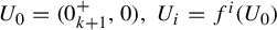 $U_0=(0^+_{k+1},0),\ U_i=f^i(U_0)$
for
$U_0=(0^+_{k+1},0),\ U_i=f^i(U_0)$
for
 $0<i\leq k+2$
,
$0<i\leq k+2$
,
 $V_0=(0,0^-_{k+2}),$
and
$V_0=(0,0^-_{k+2}),$
and
 $V_i=f^i(V_0)$
for
$V_i=f^i(V_0)$
for
 $0<i\leq k+1.$
Let us comment briefly on this definition. The mappings
 $\tilde \varphi _L$
and
$\tilde \varphi _L$
and
 $\tilde \varphi _R$
are the compositions of f corresponding to the left and right branches of the renormalization
$\tilde \varphi _R$
are the compositions of f corresponding to the left and right branches of the renormalization
 $\tilde f$
, pre-composed and post-composed with affine mappings, so that they are expressed as mappings from the unit interval onto itself. To define
$\tilde f$
, pre-composed and post-composed with affine mappings, so that they are expressed as mappings from the unit interval onto itself. To define
 $\tilde {\underline {\varphi }}_L,$
we take the direct sum of terms of the form
$\tilde {\underline {\varphi }}_L,$
we take the direct sum of terms of the form
 $\varsigma _{U_i}\underline f_L.$
Each of these terms is the restriction of (a single iterate of) f to
$\varsigma _{U_i}\underline f_L.$
Each of these terms is the restriction of (a single iterate of) f to
 $U_i$
, the ith interval in the orbit of either
$U_i$
, the ith interval in the orbit of either
 $(0,b)$
or
$(0,b)$
or
 $(b-1,0)$
, depending on whether
$(b-1,0)$
, depending on whether
 $\sigma _f = -$
or
$\sigma _f = -$
or
 $+$
, respectively, pre-composed and post-composed by affine mappings, so that it is a mapping from the unit interval onto itself. The direct sum of mappings in the decomposition space corresponds to composition of mappings, so one immediately sees that after composing the decomposed mappings we obtain
$+$
, respectively, pre-composed and post-composed by affine mappings, so that it is a mapping from the unit interval onto itself. The direct sum of mappings in the decomposition space corresponds to composition of mappings, so one immediately sees that after composing the decomposed mappings we obtain
 $\tilde f.$
As we will use the structure of Banach space in
 $\text {Diff}_{+}^{3}([0, 1])$
given by the nonlinearity operator, we need the expressions for the coordinates functions
$\text {Diff}_{+}^{3}([0, 1])$
given by the nonlinearity operator, we need the expressions for the coordinates functions
 $\tilde {\varphi }_L$
and
$\tilde {\varphi }_L$
and
 $\tilde {\varphi }_R$
in terms of the zoom operator. Note that the coordinates
$\tilde {\varphi }_R$
in terms of the zoom operator. Note that the coordinates
 $\tilde {\alpha }$
,
$\tilde {\alpha }$
,
 $\tilde {\beta }$
, and
$\tilde {\beta }$
, and
 $\tilde {b}$
remain the same as in (3.11) since they are not affected by the zoom operator. In order to obtain these coordinate functions, we need to apply the zoom operator to each branch of the first return map R on the interval
$\tilde {b}$
remain the same as in (3.11) since they are not affected by the zoom operator. In order to obtain these coordinate functions, we need to apply the zoom operator to each branch of the first return map R on the interval
 $I'= [0_{k+1}^{+}, 0_{k+2}^{-}]$
, in the case where
$I'= [0_{k+1}^{+}, 0_{k+2}^{-}]$
, in the case where
 $\sigma _f=-$
, or on the interval
$\sigma _f=-$
, or on the interval
 $I'= [0_{k+2}^{+}, 0_{k+1}^{-}]$
, in the case where
$I'= [0_{k+2}^{+}, 0_{k+1}^{-}]$
, in the case where
 $\sigma _f=+$
. Then, when
$\sigma _f=+$
. Then, when
 $\sigma _f=-$
, we obtain
$\sigma _f=-$
, we obtain
 $$ \begin{align} \tilde{\eta}_L & = Z_{[0_{k+1}^{+}, 0]} \eta_{\tilde{f}_L} = |0_{k+1}^{+}| \cdot \eta_{\tilde{f}_L} {{\kern0.5pt}\circ{\kern0.5pt}} 1_{[0_{k+1}^{+}, 0]}^{-1} = |0_{k+1}^{+}| \cdot N(f_L^k {{\kern0.5pt}\circ{\kern0.5pt}} f_R {{\kern0.5pt}\circ{\kern0.5pt}} f_L) {{\kern0.5pt}\circ{\kern0.5pt}} 1_{[0_{k+1}^{+}, 0]}^{-1},\nonumber\\ \tilde{\eta}_R & = Z_{[0, 0_{k+2}^{-}]} \eta_{\tilde{f}_R} = |0_{k+2}^{-}| \cdot \eta_{\tilde{f}_R} {{\kern0.5pt}\circ{\kern0.5pt}} 1_{[0, 0_{k+2}^{-}]}^{-1} = |0_{k+2}^{-}| \cdot N(f_L^k {{\kern0.5pt}\circ{\kern0.5pt}} f_R) {{\kern0.5pt}\circ{\kern0.5pt}} 1_{[0, 0_{k+2}^{-}]}^{-1}. \end{align} $$
The formulas when
 $\sigma =+$
are similar, and to save space we do not include them.
$\sigma =+$
are similar, and to save space we do not include them.
Remark 3.4. We would like to stress that throughout the remainder of this paper, we will make use of the Banach space structure on
 $\text {Diff}_{+}^{3}([0, 1])$
given by its identification with
$\text {Diff}_{+}^{3}([0, 1])$
given by its identification with
 $\mathcal C^1([0,1])$
via the nonlinearity operator.
$\mathcal C^1([0,1])$
via the nonlinearity operator.
4 The derivative of the renormalization operator
In this section, we will estimate the derivative of the renormalization operator acting on an absorbing set under renormalization in the decomposition space of dissipative gap mappings. A little care is needed since the operator is not differentiable.
Recall that
 $\mathcal D_0\subset \mathcal C^3$
is the set of once renormalizable dissipative gap mappings. Then
$\mathcal D_0\subset \mathcal C^3$
is the set of once renormalizable dissipative gap mappings. Then
 $\mathcal R:\mathcal D_0\to \mathcal C^2$
is differentiable, and the derivative
$\mathcal R:\mathcal D_0\to \mathcal C^2$
is differentiable, and the derivative
 $D\mathcal R_f:\mathcal C^3 \to \mathcal C^2$
extends to a bounded operator
$D\mathcal R_f:\mathcal C^3 \to \mathcal C^2$
extends to a bounded operator
 $D\mathcal R_f:\mathcal C^2\to \mathcal C^2,$
which depends continuously on
$D\mathcal R_f:\mathcal C^2\to \mathcal C^2,$
which depends continuously on
 $f\in \mathcal C^3.$
In paper [Reference Martens and Palmisano27],
$f\in \mathcal C^3.$
In paper [Reference Martens and Palmisano27],
 $\mathcal R$
is called jump-out differentiable.
$\mathcal R$
is called jump-out differentiable.
If
 $\underline {f}=(\alpha , \beta , b, \underline {\varphi }_L, \underline {\varphi }_R) \in \underline {\mathcal D}_0$
, the derivative of
$\underline {f}=(\alpha , \beta , b, \underline {\varphi }_L, \underline {\varphi }_R) \in \underline {\mathcal D}_0$
, the derivative of
 $\underline {\mathcal {R}}_{\underline {f}}$
,
$\underline {\mathcal {R}}_{\underline {f}}$
,
 $D\underline {\mathcal {R}}_{\underline {f}}$
, is a matrix of the form
$D\underline {\mathcal {R}}_{\underline {f}}$
, is a matrix of the form
 $$ \begin{align} D \underline{\mathcal{R}}_{\underline{f}} = \left( \begin{array}{@{}cc@{}} A_{\underline{f}} & B_{\underline{f}} \\ C_{\underline{f}} & D_{\underline{f}} \end{array} \right) \end{align} $$
where
-
•
$A_{\underline {f}}: \mathbb {R}^3 \rightarrow \mathbb {R}^3$
, -
•
$B_{\underline {f}}: X \times X \rightarrow \mathbb {R}^3$
, -
•
$C_{\underline {f}}: \mathbb {R}^3 \rightarrow X \times X$
, -
•
$D_{\underline {f}}: X \times X \rightarrow X \times X.$
We estimate
 $A_{\underline {f}}$
in Lemma 4.6,
$A_{\underline {f}}$
in Lemma 4.6,
 $B_{\underline {f}}$
in Lemma 4.8,
$B_{\underline {f}}$
in Lemma 4.8,
 $C_{\underline {f}}$
in Lemma 4.9, and
$C_{\underline {f}}$
in Lemma 4.9, and
 $D_{\underline {f}}$
in Lemma 4.14.
$D_{\underline {f}}$
in Lemma 4.14.
In order to estimate the entries of matrices
 $A_{\underline {f}}$
,
$A_{\underline {f}}$
,
 $B_{\underline {f}}$
,
$B_{\underline {f}}$
,
 $C_{\underline {f}}$
, and
$C_{\underline {f}}$
, and
 $D_{\underline {f}}$
, we will make use of the partial derivative operator
$D_{\underline {f}}$
, we will make use of the partial derivative operator
 $\partial $
. The main properties of
$\partial $
. The main properties of
 $\partial $
are presented in the next lemma.
$\partial $
are presented in the next lemma.
Lemma 4.1. [Reference Martens and Winckler29, Lemma 9.4]
The following equations hold whenever they make sense:
 $$ \begin{align} \partial (f {{\kern0.5pt}\circ{\kern0.5pt}} g)(x) = \partial f(g(x))+f'(g(x)) \partial g(x) , \end{align} $$
 $$ \begin{align} \partial (f^{n+1})(x) = \sum_{i=0}^{n}Df^{n-i}(f^{i+1}(x)) \partial f(f^{i}(x)), \end{align} $$
 $$ \begin{align} \partial (f^{-1})(x) = - \frac{\partial f(f^{-1}(x))}{f'(f^{-1}(x))} , \end{align} $$
 $$ \begin{align} \partial (f \cdot g)(x) = \partial f(x)g(x) +f(x)\partial g(x) , \end{align} $$
 $$ \begin{align} \partial (f/g)(x) = \frac{\partial f(x)g(x)-f(x) \partial g(x)}{(g(x))^2}. \end{align} $$
From now on, we will make use of the notation
 $$ \begin{align*} g(x) \asymp y \end{align*} $$
to mean that there exists a positive constant
 $K < \infty $
not depending on g such that
$K < \infty $
not depending on g such that
 $K^{-1}y \leq g(x) \leq K y$
, for all x in the domain of g.
$K^{-1}y \leq g(x) \leq K y$
, for all x in the domain of g.
Recall that the inverse of the nonlinearity operator
 $N: \text {Diff}_+^3([0,1]) \rightarrow \mathcal {C}^1([0,1])$
is given by
$N: \text {Diff}_+^3([0,1]) \rightarrow \mathcal {C}^1([0,1])$
is given by
 $$ \begin{align} \varphi (x) = \varphi_{\eta}(x)=N^{-1} \eta (x) = \frac{\int_0^x e^{\int_0^s \eta (t)dt}ds}{\int_0^1 e^{\int_0^s \eta (t)dt}ds}, \end{align} $$
where
 $\eta \in \mathcal {C}^1([0,1]).$
Lemma 4.2. Let
 $x \in [0, 1]$
. The evaluation operator
$x \in [0, 1]$
. The evaluation operator
 $E: \mathrm{Diff}_{+}^2([0,1]) = \mathcal {C}^0([0,1]) \rightarrow \mathbb {R}$
 $$ \begin{align*} E: \eta \mapsto \varphi_{\eta}(x) \end{align*} $$
is differentiable with derivative
 $\displaystyle {\partial \varphi (x)}/{\partial \eta }: \mathcal {C}^0([0,1]) \rightarrow \mathbb {R}$
given by
$\displaystyle {\partial \varphi (x)}/{\partial \eta }: \mathcal {C}^0([0,1]) \rightarrow \mathbb {R}$
given by
 $$ \begin{align} \displaystyle \frac{\partial \varphi (x)}{\partial \eta}(\Delta \eta ) = \bigg( \displaystyle \frac{\int_{0}^{x} \big[ \int_{0}^{s} \Delta \eta \big] e^{\int_{0}^{s} \eta }ds}{ \int_{0}^{x}e^{\int_{0}^{s}\eta} ds} - \displaystyle \frac{\int_{0}^{1} \big[ \int_{0}^{s} \Delta \eta \big] e^{\int_{0}^{s} \eta }ds}{ \int_{0}^{1}e^{\int_{0}^{s}\eta} ds}\bigg) \varphi (x). \end{align} $$
There exists
 $\varepsilon _0>0$
so that for all
$\varepsilon _0>0$
so that for all
 $\varepsilon \in (0,\varepsilon _0),$
if
$\varepsilon \in (0,\varepsilon _0),$
if
 $\| D^2\varphi \|_{\mathcal {C}^0} < \varepsilon ,$
we have that
$\| D^2\varphi \|_{\mathcal {C}^0} < \varepsilon ,$
we have that
 $$ \begin{align} \frac{1}{8}\min\{ \varphi (x), 1-\varphi (x)\}\leq \bigg| \displaystyle \frac{\partial \varphi (x)}{\partial \eta} \bigg| \leq 2 \min\{ \varphi (x), 1-\varphi (x)\}. \end{align} $$
Proof In order to prove that the evaluation operator E is (Fréchet) differentiable and obtain (4.8), we just need to use the Gateaux variation to look for a candidate T for its derivative, that is,
 $$ \begin{align} \begin{array}{@{}r@{}c@{}l} \displaystyle T(\eta) \Delta \eta &\, =\, & \displaystyle \frac{d}{dt}E(\eta + t \Delta \eta ) |_{t=0}. \\ & & \\ \end{array} \end{align} $$
Since this calculation is not difficult, we have left it to the reader. Now we will prove (4.9). Using techniques of integration, we obtain
 $$ \begin{align} \displaystyle \int_{0}^{x} \bigg[ \int_{0}^{s} \Delta \eta \bigg] e^{\int_{0}^{s} \eta }ds = \displaystyle \bigg( \int_{0}^{x} \Delta \eta \bigg) \cdot \int_{0}^{x} e^{\int_{0}^{t} \eta }ds - \int_{0}^{x} \bigg[ \Delta \eta \cdot \int_{0}^{s} e^{\int_{0}^{t} \eta } \bigg] ds. \end{align} $$
From (4.11), (4.8), and (4.7), and after some manipulations, we obtain
 $$ \begin{align} \bigg| \displaystyle \frac{\partial \varphi (x)}{\partial \eta}(\Delta \eta ) \bigg| = \varphi (x) \cdot \int_{x}^{1} \Delta \eta\, ds - \varphi (x) \cdot \int_{0}^{1} \Delta \eta \cdot \varphi(s)\, ds + \int_{0}^{x} \Delta \eta \cdot \varphi(s)\, ds. \end{align} $$
From the definition of the norm
 $$ \begin{align*} \bigg| \displaystyle \frac{\partial \varphi (x)}{\partial \eta}(\Delta \eta ) \bigg| = \sup_{\|\Delta \eta\| = 1} \bigg| \displaystyle \frac{\partial \varphi (x)}{\partial \eta} \bigg|, \end{align*} $$
we can substitute
 $\Delta \eta = 1$
into (4.12) and obtain
$\Delta \eta = 1$
into (4.12) and obtain
 $$ \begin{align*} \bigg| \displaystyle \frac{\partial \varphi (x)}{\partial \eta}(\Delta \eta ) \bigg| = \varphi (x) \cdot (1-x) - \varphi (x) \cdot \int_{0}^{1} \varphi(s)\, ds + \int_{0}^{x} \varphi(s)\, ds. \end{align*} $$
Using the fact that for deep renormalizations, the map
 $\varphi $
is close to identity, that is,
$\varphi $
is close to identity, that is,
 $\|\varphi (x) - x\|_{\mathcal C^0}$
is small, we get
$\|\varphi (x) - x\|_{\mathcal C^0}$
is small, we get
 $$ \begin{align} \bigg| \displaystyle \frac{\partial \varphi (x)}{\partial \eta}(\Delta \eta ) \bigg| & \asymp x \cdot (1-x) - x \cdot \int_{0}^{1} s\, ds + \int_{0}^{x} s\, ds \nonumber\\ & = \displaystyle \frac{x}{2} \cdot (1-x). \end{align} $$
Since
 $$ \begin{align*} \displaystyle T_{{1}/{4}}(x) \leq \frac{x}{2}(1-x) \leq T_{2}(x) \end{align*} $$
for all
 $x \in [0, 1]$
, where
$x \in [0, 1]$
, where
 $T_c(x)$
is the tent map family
$T_c(x)$
is the tent map family
 $T_c:[0,1]\to [0,1]$
, defined by
$T_c:[0,1]\to [0,1]$
, defined by
 $$ \begin{align*}T_c(x)=\left\{ \begin{array}{@{}ll} cx & \text{ for } x\in[0,1/2],\\ -cx+c & \text{ for } x\in(1/2,1]. \end{array}\right. \end{align*} $$
The result follows.
Corollary 4.3. [Reference Martens and Palmisano27, Corollary 8.17]
Let
 $\psi ^+, \psi ^- \in \mathrm{Diff}_{+}^2([0, 1])$
and
$\psi ^+, \psi ^- \in \mathrm{Diff}_{+}^2([0, 1])$
and
 $x \in [0, 1]$
. The evaluation operator
$x \in [0, 1]$
. The evaluation operator
 $$ \begin{align} \begin{array}{l@{}lll} E^{\psi_+, \psi^-} :\,\, & \mathrm{Diff}_{+}^2([0, 1]) = \mathcal{C}^0([0,1]) & \rightarrow & \mathbb{R} \\ \,\,& \eta & \mapsto & E^{\psi^+, \psi^-} (\eta) = \psi^+ {{\kern0.5pt}\circ{\kern0.5pt}} \varphi_{\eta} {{\kern0.5pt}\circ{\kern0.5pt}} \psi^- (x) \\ \end{array} \end{align} $$
is differentiable with derivative
 $\displaystyle {\partial ( \psi ^+ {{\kern0.5pt}\circ{\kern0.5pt}} \varphi _{\eta } {{\kern0.5pt}\circ{\kern0.5pt}} \psi ^- (x) ) }/{\partial \eta } : \mathcal {C}^0([0,1]) \rightarrow \mathbb {R}$
given by
$\displaystyle {\partial ( \psi ^+ {{\kern0.5pt}\circ{\kern0.5pt}} \varphi _{\eta } {{\kern0.5pt}\circ{\kern0.5pt}} \psi ^- (x) ) }/{\partial \eta } : \mathcal {C}^0([0,1]) \rightarrow \mathbb {R}$
given by
 $$ \begin{align} \displaystyle \frac{\partial ( \psi^+ {{\kern0.5pt}\circ{\kern0.5pt}} \varphi_{\eta} {{\kern0.5pt}\circ{\kern0.5pt}} \psi^- (x) ) }{\partial \eta } ( \Delta \eta ) = D \psi^+ (\varphi_{\eta} {{\kern0.5pt}\circ{\kern0.5pt}} \psi^- (x)) \cdot \frac{\partial \varphi_{\eta} (\psi^-(x))}{\partial \eta } ( \Delta \eta ). \end{align} $$
The next result follows from a straightforward calculation, and its proof is left to the reader.
Lemma 4.4. The branches
 $f_L$
and
$f_L$
and
 $f_R$
of f defined in (3.5) are differentiable and their partial derivatives are given by
$f_R$
of f defined in (3.5) are differentiable and their partial derivatives are given by
 $$ \begin{align} \begin{aligned}[b] \displaystyle \hspace{5pt}\frac{\partial f_L}{\partial \alpha }(x) & = (1-b) \cdot \displaystyle \bigg[ \varphi_L \bigg( \frac{x-b+1}{1-b} \bigg) - 1 \bigg], \quad \displaystyle \frac{\partial f_L}{\partial \beta }(x) =0, \\ \displaystyle \frac{\partial f_L}{\partial b }(x) & = 1+ \alpha \cdot \displaystyle \bigg[1- \varphi_L \bigg( \frac{x-b+1}{1-b} \bigg) \bigg] + \frac{\alpha x}{1-b} D \varphi_L \bigg( \frac{x-b+1}{1-b} \bigg), \\ \displaystyle \frac{\partial f_L}{\partial \eta_L }(x) & = \displaystyle |T_{0, L}| \cdot \frac{\partial \varphi_L (1_{I_{0, L}}^{-1}(x))}{\partial \eta_L}, \quad \displaystyle \frac{\partial f_L}{\partial \eta_R }(x) = 0, \end{aligned}\\ \begin{aligned}[b] \displaystyle &\kern-105pt\frac{\partial f_R}{\partial \alpha }(x) = 0, \quad \displaystyle \frac{\partial f_R}{\partial \beta }(x) = b \varphi_R \bigg( \frac{x}{b} \bigg),\\ \displaystyle &\kern-105pt\frac{\partial f_R}{\partial b }(x) = 1+ \beta \cdot \displaystyle \varphi_R \bigg( \frac{x}{b} \bigg) - \frac{\beta x}{b} D \varphi_R \bigg( \frac{x}{b} \bigg),\\ \displaystyle &\kern-105pt\frac{\partial f_R}{\partial \eta_L }(x) = 0, \quad \displaystyle \frac{\partial f_R}{\partial \eta_R }(x) = \displaystyle |T_{0, R}| \cdot \frac{\partial \varphi_R (1_{I_{0, R}}^{-1}(x))}{\partial \eta_R}. \end{aligned} \end{align} $$
Furthermore, all these partial derivatives are bounded.
Let
 $f=(f_L, f_R, b) \in \mathcal {D}$
be a renormalizable dissipative gap map. The boundaries of the the interval
$f=(f_L, f_R, b) \in \mathcal {D}$
be a renormalizable dissipative gap map. The boundaries of the the interval
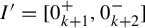 $I'=[0_{k+1}^{+}, 0_{k+2}^{-}]$
for
$I'=[0_{k+1}^{+}, 0_{k+2}^{-}]$
for
 $\sigma _f=-$
, and
$\sigma _f=-$
, and
 $I'=[0_{k+2}^{+}, 0_{k+1}^{-}]$
for
$I'=[0_{k+2}^{+}, 0_{k+1}^{-}]$
for
 $\sigma _f=+$
, can be interpreted as evaluation operators, that is,
$\sigma _f=+$
, can be interpreted as evaluation operators, that is,
 $$ \begin{align} \begin{array}{l@{}lll} E :\,\, & M & \rightarrow & \mathbb{R} \\ \,\,& (\alpha, \beta, b, \varphi_L, \varphi_R)& \mapsto & 0_{j}^{\pm} \end{array} \end{align} $$
where
 $j \in \{ k+1, k+2 \}$
depending on the sign of f. For convenience, we will call
$j \in \{ k+1, k+2 \}$
depending on the sign of f. For convenience, we will call
 $0_{j}^{\pm }$
as boundary operators. The next result gives us some properties about the boundary operators.
$0_{j}^{\pm }$
as boundary operators. The next result gives us some properties about the boundary operators.
Lemma 4.5. The boundary operators
 $0_{j}^{\pm }$
are differentiable and the partial derivatives
$0_{j}^{\pm }$
are differentiable and the partial derivatives
 $\displaystyle {\partial 0_{j}^{\pm }}/{\partial *}$
are bounded, where
$\displaystyle {\partial 0_{j}^{\pm }}/{\partial *}$
are bounded, where
 $* \in \{ \alpha , \beta , b, \eta _L, \eta _R \}$
and
$* \in \{ \alpha , \beta , b, \eta _L, \eta _R \}$
and
 $j \in \{ k+1, k+2 \}$
, depending on the sign of f.
$j \in \{ k+1, k+2 \}$
, depending on the sign of f.
Proof Consider the boundary operators
 $0_{k+2}^{-}$
and
$0_{k+2}^{-}$
and
 $0_{k+1}^{+}$
, which are explicitly given by
$0_{k+1}^{+}$
, which are explicitly given by
 $$ \begin{align*} 0_{k+1}^{+} = f_L^k(b-1) \quad \text{and} \quad 0_{k+2}^{-} = f_L^k {{\kern0.5pt}\circ{\kern0.5pt}} f_R (b), \end{align*} $$
when
 $\sigma _f=-$
, and where
$\sigma _f=-$
, and where
 $f_L = 1_{T_{0,L}} {{\kern0.5pt}\circ{\kern0.5pt}} \varphi _L {{\kern0.5pt}\circ{\kern0.5pt}} 1_{I_{0,L}}^{-1}$
and
$f_L = 1_{T_{0,L}} {{\kern0.5pt}\circ{\kern0.5pt}} \varphi _L {{\kern0.5pt}\circ{\kern0.5pt}} 1_{I_{0,L}}^{-1}$
and
 $f_R = 1_{T_{0,R}} {{\kern0.5pt}\circ{\kern0.5pt}} \varphi _R {{\kern0.5pt}\circ{\kern0.5pt}} 1_{I_{0,R}}^{-1}$
. Using (4.3) and taking
$f_R = 1_{T_{0,R}} {{\kern0.5pt}\circ{\kern0.5pt}} \varphi _R {{\kern0.5pt}\circ{\kern0.5pt}} 1_{I_{0,R}}^{-1}$
. Using (4.3) and taking
 $* \in \{ \alpha , \beta , b, \eta _L, \eta _R \}$
we get
$* \in \{ \alpha , \beta , b, \eta _L, \eta _R \}$
we get
 $$ \begin{align} \begin{array}{@{}r@{}c@{}l@{}} \displaystyle \frac{\partial }{\partial *} ( 0_{k+1}^{+} ) &\, = \displaystyle \frac{\partial}{\partial *} ( f_L^k (b-1) ) =& \displaystyle \sum_{i=0}^{k-1}Df_L^{k-1-i}(f_L^{i+1} (b-1)) \cdot \frac{\partial f_L}{\partial *} (f_L^i (b-1)), \end{array} \end{align} $$
and
 $$ \begin{align} \displaystyle \frac{\partial }{\partial *} ( 0_{k+2}^{-} ) = \displaystyle \frac{\partial}{\partial *} ( f_L^k {{\kern0.5pt}\circ{\kern0.5pt}} f_R (b) ) &= \displaystyle \sum_{i=0}^{k-1}Df_L^{k-1-i}(f_L^{i+1} {{\kern0.5pt}\circ{\kern0.5pt}} f_R(b)) \cdot \frac{\partial f_L}{\partial *} (f_L^i {{\kern0.5pt}\circ{\kern0.5pt}} f_R(b))\nonumber\\ &\quad \displaystyle +\, Df_L^k {{\kern0.5pt}\circ{\kern0.5pt}} f_R (b) \cdot \frac{\partial f_R}{\partial *}(b). \end{align} $$
Using the fact that
 $0 < f'(x) \leq \nu < 1$
, for all
$0 < f'(x) \leq \nu < 1$
, for all
 $x \in [b-1,b] \setminus \{ 0 \}$
, and Lemma 4.4, we get that
$x \in [b-1,b] \setminus \{ 0 \}$
, and Lemma 4.4, we get that
 $\displaystyle {\partial }/{\partial *} ( 0_{k+2}^{-} )$
and
$\displaystyle {\partial }/{\partial *} ( 0_{k+2}^{-} )$
and
 $\displaystyle {\partial }/{\partial *} ( 0_{k+1}^{+} )$
are bounded. With similar arguments and reasoning, we prove that the other boundary operators have bounded partial derivatives.
$\displaystyle {\partial }/{\partial *} ( 0_{k+1}^{+} )$
are bounded. With similar arguments and reasoning, we prove that the other boundary operators have bounded partial derivatives.
4.1 The
$A_{\underline {f}}$
matrix

 $$ \begin{align} A_{\underline{f}} = \left( \begin{array}{@{}ccc@{}} \displaystyle \frac{\partial \tilde{\alpha}}{\partial \alpha } & \displaystyle \frac{\partial \tilde{\alpha}}{\partial \beta } & \displaystyle \frac{\partial \tilde{\alpha}}{\partial b } \\ & & \\ \displaystyle \frac{\partial \tilde{\beta}}{\partial \alpha } & \displaystyle \frac{\partial \tilde{\beta}}{\partial \beta } & \displaystyle \frac{\partial \tilde{\beta}}{\partial b } \\ & & \\ \displaystyle \frac{\partial \tilde{b}}{\partial \alpha } & \displaystyle \frac{\partial \tilde{b}}{\partial \beta } & \displaystyle \frac{\partial \tilde{b}}{\partial b } \\ \end{array} \right). \end{align} $$
All the entries of matrix
 $A_{\underline {f}}$
can be calculated explicitly by using Lemma 4.1. In order to clarify the calculations, we will compute some of them in the next lemma.
$A_{\underline {f}}$
can be calculated explicitly by using Lemma 4.1. In order to clarify the calculations, we will compute some of them in the next lemma.
Lemma 4.6. Let
 $ \underline {f}=(\alpha ,\beta ,b,\underline {\varphi }_R, \underline {\varphi }_L) \in \underline {\mathcal D}_0$
. The map
$ \underline {f}=(\alpha ,\beta ,b,\underline {\varphi }_R, \underline {\varphi }_L) \in \underline {\mathcal D}_0$
. The map
 $$ \begin{align} \begin{array}{@{}r@{}c@{}l} (0, 1)^3 \ni (\alpha, \beta, b) &\, \mapsto\, & (\tilde{\alpha}, \tilde{\beta}, \tilde{b}) \in (0, 1)^3\\ \end{array} \end{align} $$
is differentiable. Furthermore, for any
 $\varepsilon>0, K>0$
if
$\varepsilon>0, K>0$
if
 $\underline g\in \underline {\mathcal {D}}_0$
is infinitely renormalizable, there exists
$\underline g\in \underline {\mathcal {D}}_0$
is infinitely renormalizable, there exists
 $n_0\in \mathbb N,$
so that if
$n_0\in \mathbb N,$
so that if
 $n\geq n_0$
and
$n\geq n_0$
and
 $\underline f=\underline {\mathcal {R}}^n \underline g,$
then the partial derivatives
$\underline f=\underline {\mathcal {R}}^n \underline g,$
then the partial derivatives
 $\displaystyle |({\partial }/{\partial \alpha }) \tilde {\alpha }|$
,
$\displaystyle |({\partial }/{\partial \alpha }) \tilde {\alpha }|$
,
 $\displaystyle | ({\partial }/{\partial \beta }) \tilde {\alpha }|$
,
$\displaystyle | ({\partial }/{\partial \beta }) \tilde {\alpha }|$
,
 $\displaystyle | ({\partial }/{\partial b }) \tilde {\alpha }|$
,
$\displaystyle | ({\partial }/{\partial b }) \tilde {\alpha }|$
,
 $\displaystyle | ({\partial }/{\partial \alpha }) \tilde {\beta }|$
,
$\displaystyle | ({\partial }/{\partial \alpha }) \tilde {\beta }|$
,
 $\displaystyle |({\partial }/{\partial \beta }) \tilde {\beta }|$
, and
$\displaystyle |({\partial }/{\partial \beta }) \tilde {\beta }|$
, and
 $\displaystyle |({\partial }/{\partial b }) \tilde {\beta }|$
are all bounded from above by
$\displaystyle |({\partial }/{\partial b }) \tilde {\beta }|$
are all bounded from above by
 $\varepsilon $
, and the partial derivatives
$\varepsilon $
, and the partial derivatives
 $\displaystyle |({\partial }/{\partial \alpha }) \tilde {b}|$
,
$\displaystyle |({\partial }/{\partial \alpha }) \tilde {b}|$
,
 $\displaystyle | ({\partial }/{\partial \beta }) \tilde {b}|$
and
$\displaystyle | ({\partial }/{\partial \beta }) \tilde {b}|$
and
 $\displaystyle | ({\partial }/{\partial b }) \tilde {b}|$
are bounded from below by K. In particular,
$\displaystyle | ({\partial }/{\partial b }) \tilde {b}|$
are bounded from below by K. In particular,
 $\displaystyle | ({\partial }/{\partial b }) \tilde {b}|\asymp {1}/{|I'|}.$
(See §3.3 for the definition of
$\displaystyle | ({\partial }/{\partial b }) \tilde {b}|\asymp {1}/{|I'|}.$
(See §3.3 for the definition of
 $I'$
.)
$I'$
.)
Proof We will prove this lemma in the case where
 $\sigma _f=-$
. The case
$\sigma _f=-$
. The case
 $\sigma _f=+$
is similar and we will leave it to the reader. From (3.11) we obtain the partial derivatives
$\sigma _f=+$
is similar and we will leave it to the reader. From (3.11) we obtain the partial derivatives
 $$ \begin{align} \begin{array}[c]{@{}r@{\,}c@{\,}l} \displaystyle \frac{\partial }{\partial *} \tilde{\alpha } &\; =\; & \displaystyle \frac{1}{(0_{k+1}^{+})^2} \cdot \bigg\{ 0_{k+1}^{+} \cdot \displaystyle \frac{\partial }{\partial *} ( f_L^k {{\kern0.5pt}\circ{\kern0.5pt}} f_R {{\kern0.5pt}\circ{\kern0.5pt}} f_L (0_{k+1}^{+}) ) - 0_{k+1}^{+} \cdot \displaystyle \frac{\partial }{\partial *} ( 0_{k+2}^{-} ) \\ && -\; \displaystyle [ f_L^k {{\kern0.5pt}\circ{\kern0.5pt}} f_R {{\kern0.5pt}\circ{\kern0.5pt}} f_L (0_{k+1}^{+}) - 0_{k+2}^{-} ] \cdot \displaystyle \frac{\partial }{\partial *} ( 0_{k+1}^{+} ) \bigg\}, \\ \displaystyle \frac{\partial }{\partial *} \tilde{\beta } &\; =\; & \displaystyle \frac{1}{(0_{k+2}^{-})^2} \cdot \bigg\{ 0_{k+2}^{-} \cdot \displaystyle \frac{\partial }{\partial *} ( f_L^k {{\kern0.5pt}\circ{\kern0.5pt}} f_R (0_{k+2}^{-}) ) - 0_{k+2}^{-} \cdot \displaystyle \frac{\partial }{\partial *} ( 0_{k+1}^{+} ),\\ && -\; \displaystyle [ f_L^k {{\kern0.5pt}\circ{\kern0.5pt}} f_R (0_{k+2}^{-}) - 0_{k+1}^{+} ] \cdot \displaystyle \frac{\partial }{\partial *} ( 0_{k+2}^{-} ) \bigg\} \\ \displaystyle \frac{\partial }{\partial *} \tilde{b} & \;=\; & (1-\tilde{b}) \cdot |I'|^{-1} \cdot \displaystyle \frac{\partial }{\partial *} ( f_L^k {{\kern0.5pt}\circ{\kern0.5pt}} f_R(b) ) + |I'|^{-1} \cdot \tilde{b} \cdot \displaystyle \frac{\partial }{\partial *} ( f_L^k (b-1) ),\\ \end{array} \end{align} $$
where
 $* \in \{ \alpha , \beta , b \}$
. Let us start to deal with the first line of
$* \in \{ \alpha , \beta , b \}$
. Let us start to deal with the first line of
 $A_{\underline {f}}$
, that is, with the partial derivatives
$A_{\underline {f}}$
, that is, with the partial derivatives
 $$ \begin{align*} \displaystyle \frac{\partial \tilde{\alpha}}{\partial *} \end{align*} $$
where
 $* \in \{ \alpha , \beta , b\}$
. Taking
$* \in \{ \alpha , \beta , b\}$
. Taking
 $* = \alpha $
, we obtain
$* = \alpha $
, we obtain
 $$ \begin{align} \begin{array}[b]{@{}r@{}c@{}l} \displaystyle \frac{\partial }{\partial \alpha} \tilde{\alpha } &\,=\, & \displaystyle \frac{1}{(0_{k+1}^{+})^2} \cdot \bigg\{ 0_{k+1}^{+} \cdot \displaystyle \frac{\partial }{\partial \alpha} ( f_L^k {{\kern0.5pt}\circ{\kern0.5pt}} f_R {{\kern0.5pt}\circ{\kern0.5pt}} f_L (0_{k+1}^{+}) ) - 0_{k+1}^{+} \cdot \displaystyle \frac{\partial }{\partial \alpha} ( 0_{k+2}^{-} ) \\ && -\; \displaystyle [ f_L^k {{\kern0.5pt}\circ{\kern0.5pt}} f_R {{\kern0.5pt}\circ{\kern0.5pt}} f_L (0_{k+1}^{+}) - 0_{k+2}^{-} ] \cdot \displaystyle \frac{\partial }{\partial \alpha} ( 0_{k+1}^{+} ) \bigg\}. \end{array} \end{align} $$
From (4.2) and using the fact that
 $f_R$
does not depend on
$f_R$
does not depend on
 $\alpha $
, we have
$\alpha $
, we have
 $$ \begin{align} \displaystyle \frac{\partial }{\partial \alpha} ( f_L^k {{\kern0.5pt}\circ{\kern0.5pt}} f_R {{\kern0.5pt}\circ{\kern0.5pt}} f_L (0_{k+1}^{+}) ) &\, =\, \displaystyle \frac{\partial }{\partial \alpha} ( f_L^k ) {{\kern0.5pt}\circ{\kern0.5pt}} f_R {{\kern0.5pt}\circ{\kern0.5pt}} f_L (0_{k+1}^{+})\nonumber \\ &\quad \ +\, D ( f_L^k {{\kern0.5pt}\circ{\kern0.5pt}} f_R ) {{\kern0.5pt}\circ{\kern0.5pt}} f_L(0_{k+1}^{+}) \cdot \displaystyle \frac{\partial }{\partial \alpha} ( f_L(0_{k+1}^{+}) ) \end{align} $$
Since
 $0_{k+1}^{+}=f_L^k(b-1)$
, we can apply (4.3) and get
$0_{k+1}^{+}=f_L^k(b-1)$
, we can apply (4.3) and get
 $$ \begin{align} \displaystyle \frac{\partial }{\partial \alpha} ( f_L(0_{k+1}^{+}) )\! =\! \displaystyle \frac{\partial }{\partial \alpha} ( f_L^{k+1}(b-1) )\! =\! \displaystyle \sum_{i=0}^{k} Df_L^{k-i}(f_L^{i+1}(b-1)) \cdot \displaystyle \frac{\partial f_L}{\partial \alpha} (f_L^i(b-1)). \end{align} $$
Since
 $0_{k+2}^{-} = f_L^k {{\kern0.5pt}\circ{\kern0.5pt}} f_R(b)$
by applying the mean value theorem to the difference
$0_{k+2}^{-} = f_L^k {{\kern0.5pt}\circ{\kern0.5pt}} f_R(b)$
by applying the mean value theorem to the difference
 $f_L^k {{\kern0.5pt}\circ{\kern0.5pt}} f_R {{\kern0.5pt}\circ{\kern0.5pt}} f_L (0_{k+1}^{+}) - 0_{k+2}^{-} $
, we obtain a point
$f_L^k {{\kern0.5pt}\circ{\kern0.5pt}} f_R {{\kern0.5pt}\circ{\kern0.5pt}} f_L (0_{k+1}^{+}) - 0_{k+2}^{-} $
, we obtain a point
 $\xi \in (f_L(0_{k+1}^{+}),b)$
such that
$\xi \in (f_L(0_{k+1}^{+}),b)$
such that
 $$ \begin{align} \displaystyle f_L^k {{\kern0.5pt}\circ{\kern0.5pt}} f_R {{\kern0.5pt}\circ{\kern0.5pt}} f_L (0_{k+1}^{+}) - 0_{k+2}^{-} &= f_L^k {{\kern0.5pt}\circ{\kern0.5pt}} f_R {{\kern0.5pt}\circ{\kern0.5pt}} f_L (0_{k+1}^{+})-f_L^k {{\kern0.5pt}\circ{\kern0.5pt}} f_R (b)\nonumber\\ &= D ( f_L^k {{\kern0.5pt}\circ{\kern0.5pt}} f_R )(\xi) \cdot [ f_L(0_{k+1}^{+})- b ]. \end{align} $$
Since
 $b=f_L(0^-)$
, by applying the mean value theorem once more, we obtain another point
$b=f_L(0^-)$
, by applying the mean value theorem once more, we obtain another point
 $\zeta \in (0_{k+1}^{+}, 0)$
such that
$\zeta \in (0_{k+1}^{+}, 0)$
such that
 $$ \begin{align} f_L(0_{k+1}^{+})- b = f_L(0_{k+1}^{+})- f_L(0^-) = D f_L (\zeta ) \cdot 0_{k+1}^{+}. \end{align} $$
Substituting (4.27), (4.26), and (4.24) into (4.23), and after some manipulations, we get
 $$ \begin{align} \displaystyle \frac{\partial }{\partial \alpha} \tilde{\alpha } & = \displaystyle \frac{1}{(0_{k+1}^{+})} \cdot \bigg\{ \displaystyle \frac{\partial }{\partial \alpha} ( f_L^k ) {{\kern0.5pt}\circ{\kern0.5pt}} f_R {{\kern0.5pt}\circ{\kern0.5pt}} f_L (0_{k+1}^{+}) - \displaystyle \frac{\partial }{\partial \alpha} ( f_L^k ) {{\kern0.5pt}\circ{\kern0.5pt}} f_R(b) \nonumber\\ & \quad + D(f_L^k {{\kern0.5pt}\circ{\kern0.5pt}} f_R) {{\kern0.5pt}\circ{\kern0.5pt}} f_L(0_{k+1}^{+}) \cdot \displaystyle \frac{\partial }{\partial \alpha} ( f_L(0_{k+1}^{+}) ) \nonumber\\ & \quad - \displaystyle [ D ( f_L^k {{\kern0.5pt}\circ{\kern0.5pt}} f_R )(\xi) \cdot D f_L (\zeta ) ] \cdot \displaystyle \frac{\partial }{\partial \alpha} ( 0_{k+1}^{+} ) \bigg\}. \end{align} $$
By (4.3), we obtain
 $$ \begin{align} &\displaystyle \frac{\partial }{\partial \alpha} ( f_L^k ) {{\kern0.5pt}\circ{\kern0.5pt}} f_R {{\kern0.5pt}\circ{\kern0.5pt}} f_L (0_{k+1}^{+}) - \frac{\partial }{\partial \alpha} ( f_L^k ) {{\kern0.5pt}\circ{\kern0.5pt}} f_R (b) \nonumber\\ &\quad= \displaystyle \sum_{i=0}^{k-1}Df_L^{k-1-i} ( f_L^{i+1} {{\kern0.5pt}\circ{\kern0.5pt}} f_R {{\kern0.5pt}\circ{\kern0.5pt}} f_L(0_{k+1}^{+})) \cdot \displaystyle \frac{\partial f_L}{\partial \alpha}( f_L^i {{\kern0.5pt}\circ{\kern0.5pt}} f_R {{\kern0.5pt}\circ{\kern0.5pt}} f_L(0_{k+1}^{+})) \nonumber\\ &\quad\quad- \displaystyle \sum_{i=0}^{k-1}Df_L^{k-1-i} ( f_L^{i+1} {{\kern0.5pt}\circ{\kern0.5pt}} f_R(b)) \cdot \displaystyle \frac{\partial f_L}{\partial \alpha} ( f_L^i {{\kern0.5pt}\circ{\kern0.5pt}} f_R (b)). \end{align} $$
From Lemma 4.4, we know that
 $\displaystyle ({\partial f_L}/{\partial \alpha })(x)$
is bounded, then putting
$\displaystyle ({\partial f_L}/{\partial \alpha })(x)$
is bounded, then putting
 $$ \begin{align*} C_1 = \max_{0 \leq i < k } \bigg\{ \displaystyle \bigg| \frac{\partial f_L}{\partial \alpha }(f_L^i {{\kern0.5pt}\circ{\kern0.5pt}} f_R {{\kern0.5pt}\circ{\kern0.5pt}} f_L(0_{k+1}^{+})) \bigg|, \bigg| \frac{\partial f_L}{\partial \alpha }(f_L^i {{\kern0.5pt}\circ{\kern0.5pt}} f_R (b)) \bigg| \bigg\}, \end{align*} $$
we obtain
 $$ \begin{align} &\displaystyle \bigg| \frac{\partial }{\partial \alpha} ( f_L^k ) {{\kern0.5pt}\circ{\kern0.5pt}} f_R {{\kern0.5pt}\circ{\kern0.5pt}} f_L (0_{k+1}^{+}) - \frac{\partial }{\partial \alpha} ( f_L^k ) {{\kern0.5pt}\circ{\kern0.5pt}} f_R (b) \bigg| \nonumber\\ &\quad\leq C_1 \cdot \displaystyle \sum_{i=0}^{k-1} \bigg| Df_L^{k-1-i} ( f_L^{i+1} {{\kern0.5pt}\circ{\kern0.5pt}} f_R {{\kern0.5pt}\circ{\kern0.5pt}} f_L(0_{k+1}^{+})) - Df_L^{k-1-i} ( f_L^{i+1} {{\kern0.5pt}\circ{\kern0.5pt}} f_R(b)) \bigg|. \end{align} $$
Applying the mean value theorem twice, we obtain a point
 $\xi _i \in (f_{L}^{i+1} {{\kern0.5pt}\circ{\kern0.5pt}} f_R {{\kern0.5pt}\circ{\kern0.5pt}} f_L(0_{k+1}^{+}), f_{L}^{i+1} {{\kern0.5pt}\circ{\kern0.5pt}} f_R(b))$
, and a point
$\xi _i \in (f_{L}^{i+1} {{\kern0.5pt}\circ{\kern0.5pt}} f_R {{\kern0.5pt}\circ{\kern0.5pt}} f_L(0_{k+1}^{+}), f_{L}^{i+1} {{\kern0.5pt}\circ{\kern0.5pt}} f_R(b))$
, and a point
 $\theta _i \in (f_L(0_{k+1}^{+}), b)$
such that
$\theta _i \in (f_L(0_{k+1}^{+}), b)$
such that
 $$ \begin{align} &| Df_L^{k-1-i} ( f_L^{i+1} {{\kern0.5pt}\circ{\kern0.5pt}} f_R {{\kern0.5pt}\circ{\kern0.5pt}} f_L(0_{k+1}^{+})) - Df_L^{k-1-i} ( f_L^{i+1} {{\kern0.5pt}\circ{\kern0.5pt}} f_R(b)) | \notag \\ &\quad= | D^2 f_L^{k-1-i}(\xi_i)| \cdot | D(f_L^{i+1} {{\kern0.5pt}\circ{\kern0.5pt}} f_R) (\theta_i)| \cdot | Df_L(\zeta)| \cdot |0_{k+1}^{+}|. \end{align} $$
From this we obtain
 $$ \begin{align} &\displaystyle \bigg| \frac{\partial }{\partial \alpha} ( f_L^k ) {{\kern0.5pt}\circ{\kern0.5pt}} f_R {{\kern0.5pt}\circ{\kern0.5pt}} f_L (0_{k+1}^{+}) - \frac{\partial }{\partial \alpha} ( f_L^k ) {{\kern0.5pt}\circ{\kern0.5pt}} f_R (b) \bigg|\notag \\ &\quad\leq C_1 \cdot |0_{k+1}^{+}| \cdot \displaystyle \sum_{i=0}^{k-1} | D^2 f_L^{k-1-i}(\xi_i)| \cdot | D(f_L^{i+1} {{\kern0.5pt}\circ{\kern0.5pt}} f_R) (\theta_i)| \cdot | Df_L(\zeta)|\notag \\ &\quad= C_1 \cdot |0_{k+1}^{+}| \cdot | Df_L(\zeta)| \cdot \displaystyle \sum_{i=0}^{k-1} | D^2 f_L^{k-1-i}(\xi_i)| \notag\\ &\quad\quad\cdot\; | Df_L^{i} {{\kern0.5pt}\circ{\kern0.5pt}} f_L {{\kern0.5pt}\circ{\kern0.5pt}} f_R (\theta_i)| \cdot | Df_L {{\kern0.5pt}\circ{\kern0.5pt}} f_R (\theta_i) | \cdot | Df_R(\theta_i) |. \end{align} $$
For the other difference in (4.28), we start by observing that
 $\displaystyle ({\partial }/{\partial \alpha }) ( f_L(0_{k+1}^{+}))$
and
$\displaystyle ({\partial }/{\partial \alpha }) ( f_L(0_{k+1}^{+}))$
and
 $\displaystyle ({\partial }/{\partial \alpha }) ( 0_{k+1}^{+} )$
are either simultaneously positive or negative. Furthermore, from Lemma 4.5, we have that
$\displaystyle ({\partial }/{\partial \alpha }) ( 0_{k+1}^{+} )$
are either simultaneously positive or negative. Furthermore, from Lemma 4.5, we have that
 $\displaystyle ({\partial }/{\partial \alpha }) ( 0_{k+1}^{+} )$
is bounded, and arguing similarly, we have that
$\displaystyle ({\partial }/{\partial \alpha }) ( 0_{k+1}^{+} )$
is bounded, and arguing similarly, we have that
 $\displaystyle {\partial }/{\partial \alpha } ( f_L(0_{k+1}^{+}))$
is also bounded. Thus, there exists a constant
$\displaystyle {\partial }/{\partial \alpha } ( f_L(0_{k+1}^{+}))$
is also bounded. Thus, there exists a constant
 $\displaystyle C_2>0$
such that
$\displaystyle C_2>0$
such that
 $$ \begin{align} &\bigg| \displaystyle D(f_L^k {{\kern0.5pt}\circ{\kern0.5pt}} f_R) {{\kern0.5pt}\circ{\kern0.5pt}} f_L(0_{k+1}^{+}) \cdot \frac{\partial }{\partial \alpha} ( f_L(0_{k+1}^{+})) - \displaystyle [ D ( f_L^k {{\kern0.5pt}\circ{\kern0.5pt}} f_R )(\xi) \cdot D f_L (\zeta ) ] \cdot \displaystyle \frac{\partial }{\partial \alpha} ( 0_{k+1}^{+} ) \bigg| \notag\\ &\quad\leq C_2 \cdot | D(f_L^k {{\kern0.5pt}\circ{\kern0.5pt}} f_R) {{\kern0.5pt}\circ{\kern0.5pt}} f_L(0_{k+1}^{+}) - D(f_L^k {{\kern0.5pt}\circ{\kern0.5pt}} f_R) (\xi) | \notag\\ &\quad\leq C_2 \cdot | D^2(f_L^k {{\kern0.5pt}\circ{\kern0.5pt}} f_R)(w)| \cdot | Df_L (\zeta) | \cdot |0_{k+1}^{+}| \end{align} $$
where
 $w \in (f_L(0_{k+1}^{+}), \xi )$
is a point given by the mean value theorem.
$w \in (f_L(0_{k+1}^{+}), \xi )$
is a point given by the mean value theorem.
Substituting (4.32) and (4.33) into (4.28), we obtain
 $$ \begin{align} \displaystyle \bigg| \frac{\partial }{\partial \alpha} \tilde{\alpha}\bigg| & \leq C_1 \cdot | Df_L(\zeta)| \cdot \displaystyle \sum_{i=0}^{k-1} | D^2 f_L^{k-1-i}(\xi_i)| \cdot | Df_L^{i} {{\kern0.5pt}\circ{\kern0.5pt}} f_L {{\kern0.5pt}\circ{\kern0.5pt}} f_R (\theta_i)| \notag\\ & \quad\cdot\; | Df_L {{\kern0.5pt}\circ{\kern0.5pt}} f_R (\theta_i) | \cdot | Df_R(\theta_i) | + C_2 \cdot | D^2(f_L^k {{\kern0.5pt}\circ{\kern0.5pt}} f_R)(w)| \cdot | Df_L (\zeta) |. \end{align} $$
Since the first and second derivatives of f go to zero when the level of renormalization goes to infinity, we conclude that
 $ \displaystyle | ({\partial }/{\partial \alpha }) \tilde {\alpha } | \longrightarrow 0$
when the level of renormalization goes to infinity. With same arguments and reasoning, we can prove that
$ \displaystyle | ({\partial }/{\partial \alpha }) \tilde {\alpha } | \longrightarrow 0$
when the level of renormalization goes to infinity. With same arguments and reasoning, we can prove that
 $\displaystyle | ({\partial }/{\partial \beta }) \tilde {\alpha } |$
,
$\displaystyle | ({\partial }/{\partial \beta }) \tilde {\alpha } |$
,
 $\displaystyle | ({\partial }/{\partial b}) \tilde {\alpha } |$
,
$\displaystyle | ({\partial }/{\partial b}) \tilde {\alpha } |$
,
 $\displaystyle | ({\partial }/{\partial \alpha }) \tilde {\beta } |$
,
$\displaystyle | ({\partial }/{\partial \alpha }) \tilde {\beta } |$
,
 $\displaystyle | ({\partial }/{\partial \beta }) \tilde {\beta } |$
, and
$\displaystyle | ({\partial }/{\partial \beta }) \tilde {\beta } |$
, and
 $\displaystyle | ({\partial }/{\partial b}) \tilde {\beta } |$
all tend to zero as the level of renormalization tends to infinity.
$\displaystyle | ({\partial }/{\partial b}) \tilde {\beta } |$
all tend to zero as the level of renormalization tends to infinity.
Now we will prove that
 $\displaystyle | {\partial \tilde {b} }/{\partial b} |$
is big. From (4.22), we have
$\displaystyle | {\partial \tilde {b} }/{\partial b} |$
is big. From (4.22), we have
 $$ \begin{align} \displaystyle \bigg| \frac{\partial \tilde{b}}{\partial b} \bigg| & = \displaystyle \frac{1}{|I'|^2} \cdot \bigg\{ 0_{k+2}^{-} \cdot \frac{\partial }{\partial b} ( 0_{k+1}^{+} ) - 0_{k+1}^{+} \cdot \frac{\partial }{\partial b} ( 0_{k+2}^{-} ) \bigg\} \notag\\ & \geq \displaystyle \frac{1}{|I'|} \cdot \text{min} \bigg\{ \frac{\partial }{\partial b} ( 0_{k+1}^{+} ), \frac{\partial }{\partial b} ( 0_{k+2}^{-} ) \bigg\} \notag \\ & \geq \displaystyle \frac{1}{|I'|} \cdot \text{min} \bigg\{ \frac{\partial f_L}{\partial b} ( f_L^{k-1}(b-1) ), \frac{\partial f_L}{\partial b} ( f_L^{k-1} {{\kern0.5pt}\circ{\kern0.5pt}} f_R(b) ) \bigg\} \end{align} $$
which is big since the size of
 $I'$
goes to 0 when the level of renormalization is deeper, and from Lemma 4.4 we get that
$I'$
goes to 0 when the level of renormalization is deeper, and from Lemma 4.4 we get that
 $\displaystyle ({\partial f_L}/{\partial b}) ( f_L^{k-1} {{\kern0.5pt}\circ{\kern0.5pt}} f_R(b) )$
and
$\displaystyle ({\partial f_L}/{\partial b}) ( f_L^{k-1} {{\kern0.5pt}\circ{\kern0.5pt}} f_R(b) )$
and
 $\displaystyle ({\partial f_L}/{\partial b}) ( f_L^{k-1}(b-1) )$
are both greater than a positive constant
$\displaystyle ({\partial f_L}/{\partial b}) ( f_L^{k-1}(b-1) )$
are both greater than a positive constant
 $c>1/3$
. With the same arguments, we prove that
$c>1/3$
. With the same arguments, we prove that
 $\displaystyle | {\partial \tilde {b} }/{\partial \alpha } |$
and
$\displaystyle | {\partial \tilde {b} }/{\partial \alpha } |$
and
 $\displaystyle | {\partial \tilde {b} }/{\partial \beta } |$
are big.
$\displaystyle | {\partial \tilde {b} }/{\partial \beta } |$
are big.
Remark 4.7. We note that all the calculations used to get
 $({\partial \tilde {\alpha }}/{\partial \alpha })(x)$
in the above proof of Lemma 4.6 we can use to get the others partial derivatives
$({\partial \tilde {\alpha }}/{\partial \alpha })(x)$
in the above proof of Lemma 4.6 we can use to get the others partial derivatives
 $({\partial \tilde {\alpha }}/{\partial \beta })(x)$
,
$({\partial \tilde {\alpha }}/{\partial \beta })(x)$
,
 $ ({\partial \tilde {\alpha }}/{\partial b })(x)$
,
$ ({\partial \tilde {\alpha }}/{\partial b })(x)$
,
 ${\partial \tilde {\alpha }}/{\partial \eta _L} $
, and
${\partial \tilde {\alpha }}/{\partial \eta _L} $
, and
 $({\partial \tilde {\alpha }}/{\partial \eta _R })(x)$
, just observing that in each case the constants will depend on the specific partial derivative we are calculating, that is, in the calculation of
$({\partial \tilde {\alpha }}/{\partial \eta _R })(x)$
, just observing that in each case the constants will depend on the specific partial derivative we are calculating, that is, in the calculation of
 $({\partial \tilde {\alpha }}/{\partial \eta _L })(x)$
the constants
$({\partial \tilde {\alpha }}/{\partial \eta _L })(x)$
the constants
 $C_1$
and
$C_1$
and
 $C_2$
will depend on
$C_2$
will depend on
 ${\partial f_L}/{\partial \eta _L }$
.
${\partial f_L}/{\partial \eta _L }$
.
4.2 The
$B_{\underline {f}}$
matrix

 $$ \begin{align} B_{\underline{f}} = \left( \begin{array}{@{}cc@{}} \displaystyle \frac{\partial \tilde{\alpha}}{\partial \eta_L } & \displaystyle \frac{\partial \tilde{\alpha}}{\partial \eta_R } \\ & \\ \displaystyle \frac{\partial \tilde{\beta}}{\partial \eta_L } & \displaystyle \frac{\partial \tilde{\beta}}{\partial \eta_R } \\ & \\ \displaystyle \frac{\partial \tilde{b}}{\partial \eta_L } & \displaystyle \frac{\partial \tilde{b}}{\partial \eta_R } \\ \end{array} \right). \end{align} $$
Lemma 4.8. Let
 $\underline {f} \in \underline {\mathcal D}_0$
. The maps
$\underline {f} \in \underline {\mathcal D}_0$
. The maps
 $$ \begin{align}\begin{aligned} {\mathcal C}^1([0, 1]) \ni \eta_L & \mapsto (\tilde{\alpha}, \tilde{\beta}, \tilde{b}) \in (0, 1)^3, \\ {\mathcal C}^1([0, 1]) \ni \eta_R & \mapsto (\tilde{\alpha}, \tilde{\beta}, \tilde{b}) \in (0, 1)^3 \end{aligned}\end{align} $$
are differentiable. Moreover, for any
 $\varepsilon>0$
, if
$\varepsilon>0$
, if
 $\underline g\in \underline {\mathcal {D}}$
is infinitely renormalizable, and
$\underline g\in \underline {\mathcal {D}}$
is infinitely renormalizable, and
 $\underline f=\underline {\mathcal {R}}^n\underline g$
, then there exists
$\underline f=\underline {\mathcal {R}}^n\underline g$
, then there exists
 $n_0\in \mathbb N$
so that for
$n_0\in \mathbb N$
so that for
 $n\geq n_0$
, we have that
$n\geq n_0$
, we have that
 $\displaystyle | {\partial \tilde {\alpha }}/{\partial \eta _L }|, \displaystyle |{\partial \tilde {\alpha }}/{\partial \eta _R }|, \displaystyle | {\partial \tilde {\beta }}/{\partial \eta _L }|, \displaystyle |{\partial \tilde {\beta }}/{\partial \eta _R }|<\varepsilon $
,
$\displaystyle | {\partial \tilde {\alpha }}/{\partial \eta _L }|, \displaystyle |{\partial \tilde {\alpha }}/{\partial \eta _R }|, \displaystyle | {\partial \tilde {\beta }}/{\partial \eta _L }|, \displaystyle |{\partial \tilde {\beta }}/{\partial \eta _R }|<\varepsilon $
,
 $\displaystyle |{\partial \tilde {b}}/{\partial \eta _R }|=0,$
and
$\displaystyle |{\partial \tilde {b}}/{\partial \eta _R }|=0,$
and
 $\displaystyle | {\partial \tilde {b}}/{\partial \eta _L }|\asymp {b}/{|I'|}$
, where
$\displaystyle | {\partial \tilde {b}}/{\partial \eta _L }|\asymp {b}/{|I'|}$
, where
 $I'$
is as defined in §3.3.
$I'$
is as defined in §3.3.
Proof From (3.11), the expressions of the partial derivatives of
 $\tilde {\alpha }$
,
$\tilde {\alpha }$
,
 $\tilde {\beta }$
, and
$\tilde {\beta }$
, and
 $\tilde {b}$
are given by
$\tilde {b}$
are given by
 $$ \begin{align} \begin{aligned} \displaystyle \frac{\partial }{\partial *} \tilde{\alpha } & = \displaystyle \frac{1}{(0_{k+1}^{+})^2} \cdot \bigg\{ 0_{k+1}^{+} \cdot \displaystyle \frac{\partial }{\partial *} ( f_L^k \circ f_R \circ f_L (0_{k+1}^{+}) ) - 0_{k+1}^{+} \cdot \displaystyle \frac{\partial }{\partial *} ( 0_{k+2}^{-} ) \\ & \quad \,-\; \displaystyle [ f_L^k \circ f_R \circ f_L (0_{k+1}^{+}) - 0_{k+2}^{-} ] \cdot \displaystyle \frac{\partial }{\partial *} ( 0_{k+1}^{+} ) \bigg\}, \\ \displaystyle \frac{\partial }{\partial *} \tilde{\beta } & = \displaystyle \frac{1}{(0_{k+2}^{-})^2} \cdot \bigg\{ 0_{k+2}^{-} \cdot \displaystyle \frac{\partial }{\partial *} ( f_L^k \circ f_R (0_{k+2}^{-}) ) - 0_{k+2}^{-} \cdot \displaystyle \frac{\partial }{\partial *} ( 0_{k+1}^{+} ) \\ &\quad\, -\;\displaystyle [ f_L^k \circ f_R (0_{k+2}^{-}) - 0_{k+1}^{+} ] \cdot \displaystyle \frac{\partial }{\partial *} ( 0_{k+2}^{-} ) \bigg\},\\ \displaystyle \frac{\partial }{\partial *} \tilde{b} & = (1-\tilde{b}) \cdot |I'|^{-1} \cdot \displaystyle \frac{\partial }{\partial *} ( f_L^k \circ f_R(b) ) + |I'|^{-1} \cdot \tilde{b} \cdot \displaystyle \frac{\partial }{\partial *} ( f_L^k (b-1) ), \end{aligned} \end{align} $$
where
 $* \in \{ \eta _L, \eta _R \}$
. With similar arguments used in the proof of Lemma 4.6, we can prove that
$* \in \{ \eta _L, \eta _R \}$
. With similar arguments used in the proof of Lemma 4.6, we can prove that
 $$ \begin{align*} \displaystyle \frac{\partial \tilde{\alpha}}{\partial \eta_L}, \;\; \frac{\partial \tilde{\alpha}}{\partial \eta_R}, \;\; \frac{\partial \tilde{\beta}}{\partial \eta_L}, \;\; \frac{\partial \tilde{\beta}}{\partial \eta_R} \end{align*} $$
are as small as we want.
Now let us estimate
 $$ \begin{align*} \displaystyle \frac{\partial }{\partial \eta_L} \tilde{b} \quad \text{and} \quad \frac{\partial }{\partial \eta_R} \tilde{b}. \end{align*} $$
Observe that at deep levels of renormalization, the diffeomorphic parts
 $\varphi _L$
and
$\varphi _L$
and
 $\varphi _R$
are very close to the identity function, so we can assume that
$\varphi _R$
are very close to the identity function, so we can assume that
 $$ \begin{align*} \varphi_L(x) = x + o(\epsilon), \quad \varphi_R(x) = x + o(\epsilon) \end{align*} $$
where
 $\epsilon>0$
is arbitrarily small. With some manipulations, we get from (4.38)
$\epsilon>0$
is arbitrarily small. With some manipulations, we get from (4.38)
 $$ \begin{align} \displaystyle \frac{\partial }{\partial \eta_L} \tilde{b} & = \displaystyle \frac{1}{|I'|^2} \cdot \bigg\{ 0_{k+2}^{-} \cdot \frac{\partial }{\partial \eta_L} ( 0_{k+1}^{+} ) -0_{k+1}^{+} \cdot \frac{\partial }{\partial \eta_L} ( 0_{k+2}^{-}) \bigg\}. \end{align} $$
Let us analyze each term inside the braces separately. Since
 $$ \begin{align*}0_{k+1}^{+} = f_L^k(b-1) = f_L (f_L^{k-1}(b-1))\text{ and }f_L = 1_{T_{0,L}} {{\kern0.5pt}\circ{\kern0.5pt}} \varphi_L {{\kern0.5pt}\circ{\kern0.5pt}} 1_{I_{0,L}}^{-1},\end{align*} $$
we obtain
 $$ \begin{align} \displaystyle \frac{\partial }{\partial \eta_L} ( 0_{k+1}^{+} ) & = \displaystyle \frac{\partial }{\partial \eta_L} ( f_L (f_L^{k-1}(b-1)) ) \notag \\[5pt] & = D 1_{T_{0,L}} {{\kern0.5pt}\circ{\kern0.5pt}} ( \varphi_L {{\kern0.5pt}\circ{\kern0.5pt}} 1_{I_{0,L}}^{-1} {{\kern0.5pt}\circ{\kern0.5pt}} f_L^{k-1}(b-1) ) \cdot \displaystyle \frac{\partial }{\partial \eta_L} ( \varphi_L {{\kern0.5pt}\circ{\kern0.5pt}} 1_{I_{0,L}}^{-1} (f_L^{k-1}(b-1)) ) \notag \\[5pt] & \asymp |T_{0,L}| \cdot \min\{ \varphi_L {{\kern0.5pt}\circ{\kern0.5pt}} 1_{I_{0,L}}^{-1} (f_L^{k-1}(b-1)), 1- \varphi_L {{\kern0.5pt}\circ{\kern0.5pt}} 1_{I_{0,L}}^{-1} (f_L^{k-1}(b-1)) \}\notag \\[5pt] & \asymp |T_{0,L}| \cdot \min\{ 1_{I_{0,L}}^{-1} (f_L^{k-1}(b-1)), 1- 1_{I_{0,L}}^{-1} (f_L^{k-1}(b-1)) \} \notag\\[5pt] & = |T_{0,L}| \cdot (1-1_{I_{0,L}}^{-1} (f_L^{k-1}(b-1)) ). \end{align} $$
By using analogous arguments, we get
 $$ \begin{align} \displaystyle \frac{\partial }{\partial \eta_L} ( 0_{k+2}^{-} ) & = \displaystyle \frac{\partial }{\partial \eta_L} ( f_L (f_L^{k-1}(f_R(b))) )\notag\\[5pt] & \asymp |T_{0,L}| \cdot (1-1_{I_{0,L}}^{-1} (f_L^{k-1}(f_R(b))) ). \end{align} $$
Substituting (4.41) and (4.40) into (4.39), we get
 $$ \begin{align} \displaystyle \frac{\partial }{\partial \eta_L} \tilde{b} & \! \asymp \displaystyle \frac{|T_{0,L}|}{|I'|^2}\! \cdot\! \{ 0_{k+2}^{-} \!\cdot\! (1-1_{I_{0,L}}^{-1} (f_L^{k-1}(b-1)) )\! - \! 0_{k+1}^{+} \cdot (1-1_{I_{0,L}}^{-1} (f_L^{k-1}(f_R(b))) ) \}\notag\\[5pt] & = \displaystyle \frac{|T_{0,L}|}{|I'|^2} \cdot [ 0_{k+2}^{-} - 0_{k+1}^{+} ] + \displaystyle \frac{|T_{0,L}|}{|I'|^2} \cdot 0_{k+1}^{+} \cdot 1_{I_{0,L}}^{-1} (f_L^{k-1}(f_R(b))) \notag \\[5pt] & \quad- \displaystyle \frac{ |T_{0,L}| }{|I'|^2} \cdot 0_{k+2}^{-} \cdot 1_{I_{0,L}}^{-1} (f_L^{k-1}(b-1)). \end{align} $$
Since the size of the renormalization interval
 $I'$
goes to zero when the level of renormalization goes to infinity, we can assume that
$I'$
goes to zero when the level of renormalization goes to infinity, we can assume that
 $b-0_{k+2}^{-} \asymp b$
, and then we have
$b-0_{k+2}^{-} \asymp b$
, and then we have
 $$ \begin{align} |0_{k+1}^{-}|=0-f_L^{k-1}(f_R(b)) = \frac{b-0_{k+2}^{-}}{Df_L(c_1)} \asymp \frac{b}{Df_L(c_1)} \asymp b \cdot \frac{|I_{0,L}|}{|T_{0,L}|}, \end{align} $$
where we use the assumption that
 $$ \begin{align} \left. \begin{array}{@{}r@{}c@{}l} f_L &\; = \; & 1_{T_{0,L}} {{\kern0.5pt}\circ{\kern0.5pt}} \varphi_L {{\kern0.5pt}\circ{\kern0.5pt}} 1_{I_{0,L}}^{-1} \\ \varphi_L & \; \approx \; & \text{identity function} \\ \end{array} \right\} \Rightarrow Df_L = \frac{|T_{0,L}|}{|I_{0,L}|} \cdot D \varphi_L \asymp \frac{|T_{0,L}|}{|I_{0,L}|}. \end{align} $$
By using the approximation (4.44), we have
 $$ \begin{align} |0_{k}^{+}|=0-f_L^{k-1}(b-1) = \frac{b-0_{k+1}^{+}}{Df_L(c_2)} \asymp (b-0_{k+1}^{+}) \cdot \frac{|I_{0,L}|}{|T_{0,L}|}. \end{align} $$
Using (4.45), (4.44), and the definition of the affine map
 $1_{I_{0,L}}^{-1}$
by (4.42), we obtain
$1_{I_{0,L}}^{-1}$
by (4.42), we obtain
 $$ \begin{align} \displaystyle \frac{\partial }{\partial \eta_L} \tilde{b} \asymp \displaystyle \frac{-b}{|I'|} + \frac{0_{k+1}^{+} \cdot 0_{k+2}^{-}}{|I'|^2}. \end{align} $$
Since
 $I'= [0_{k+1}^{+}, 0_{k+2}^{-}]$
and
$I'= [0_{k+1}^{+}, 0_{k+2}^{-}]$
and
 $|I'| \leq \alpha \cdot \beta \cdot b$
for all
$|I'| \leq \alpha \cdot \beta \cdot b$
for all
 $k \geq 1$
, we can conclude that
$k \geq 1$
, we can conclude that
 $\displaystyle ({0_{k+1}^{+} \cdot 0_{k+2}^{-}})/{|I'|^2}$
is bounded and thus
$\displaystyle ({0_{k+1}^{+} \cdot 0_{k+2}^{-}})/{|I'|^2}$
is bounded and thus
 $\displaystyle | ({\partial }/{\partial \eta _L}) \tilde {b} | \asymp {-b}/{|I'|}.$
For the derivative of
$\displaystyle | ({\partial }/{\partial \eta _L}) \tilde {b} | \asymp {-b}/{|I'|}.$
For the derivative of
 $\tilde {b}$
with respect to
$\tilde {b}$
with respect to
 $\eta _R$
, we start by noting that
$\eta _R$
, we start by noting that
 $0_{k+1}^{+} = f_L^{k}(b-1)$
does not depend on
$0_{k+1}^{+} = f_L^{k}(b-1)$
does not depend on
 $\eta _R$
. Hence, with similar arguments used to get (4.39), we obtain
$\eta _R$
. Hence, with similar arguments used to get (4.39), we obtain
 $$ \begin{align} \displaystyle \frac{\partial }{\partial \eta_R} \tilde{b} & = \displaystyle \frac{1}{|I'|^2} \cdot \bigg\{ 0_{k+2}^{-} \cdot \frac{\partial }{\partial \eta_R} ( 0_{k+1}^{+} ) -0_{k+1}^{+} \cdot \frac{\partial }{\partial \eta_R} ( 0_{k+2}^{-}) \bigg\} \nonumber\\ & = \displaystyle \frac{-0_{k+1}^{+}}{|I'|^2} \cdot Df_L^k {{\kern0.5pt}\circ{\kern0.5pt}} f_R (b) \cdot \frac{\partial }{\partial \eta_R} ( f_R(b) ). \end{align} $$
Since
 $\displaystyle f_R = 1_{T_{o,R}} {{\kern0.5pt}\circ{\kern0.5pt}} \varphi _R {{\kern0.5pt}\circ{\kern0.5pt}} 1_{I_{0,R}}^{-1}$
and the point
$\displaystyle f_R = 1_{T_{o,R}} {{\kern0.5pt}\circ{\kern0.5pt}} \varphi _R {{\kern0.5pt}\circ{\kern0.5pt}} 1_{I_{0,R}}^{-1}$
and the point
 $1_{I_{0,R}}^{-1}(b)$
is always fixed by any
$1_{I_{0,R}}^{-1}(b)$
is always fixed by any
 $\varphi _R \in \text {Diff}_{+}^{3}[0,1]$
, we obtain
$\varphi _R \in \text {Diff}_{+}^{3}[0,1]$
, we obtain
 $$ \begin{align*} \displaystyle \frac{\partial }{\partial \eta_R} ( \varphi_R {{\kern0.5pt}\circ{\kern0.5pt}} 1_{I_{0,R}}^{-1}(b) ) =0 \end{align*} $$
and then
 $$ \begin{align*} \displaystyle \frac{\partial }{\partial \eta_R} ( f_R(b) ) = D1_{T_{0,R}} {{\kern0.5pt}\circ{\kern0.5pt}} ( \varphi_R {{\kern0.5pt}\circ{\kern0.5pt}} 1_{I_{0,R}}^{-1}(b) ) \cdot \frac{\partial }{\partial \eta_R} ( \varphi_R {{\kern0.5pt}\circ{\kern0.5pt}} 1_{I_{0,R}}^{-1}(b) ) = 0 \end{align*} $$
which implies in
 $$ \begin{align*} \displaystyle \frac{\partial }{\partial \eta_R} \tilde{b}=0 \end{align*} $$
as desired.
4.3 The
$C_{\underline {f}}$
matrix

 $$ \begin{align} C_{\underline{f}} = \left( \begin{array}{@{}ccc@{}} \displaystyle \frac{\partial \tilde{\eta}_L}{\partial \alpha } & \displaystyle \frac{\partial \tilde{\eta}_L}{\partial \beta } & \displaystyle \frac{\partial \tilde{\eta}_L}{\partial b } \\[-5pt] & & \\ \displaystyle \frac{\partial \tilde{\eta}_R}{\partial \alpha } & \displaystyle \frac{\partial \tilde{\eta}_R}{\partial \beta } & \displaystyle \frac{\partial \tilde{\eta}_R}{\partial b } \end{array} \right). \end{align} $$
Lemma 4.9. Let
 $ \underline {f} \in \underline {\mathcal D}_0 $
. The maps
$ \underline {f} \in \underline {\mathcal D}_0 $
. The maps
 $$ \begin{align}\begin{aligned} (0,1)^3 \ni (\alpha, \beta, b) & \mapsto \tilde{\eta}_L \in {\mathcal C}^{1}([0, 1]), \\ {(0, 1)^3} \ni (\alpha, \beta, b) & \mapsto \tilde{\eta}_R \in {\mathcal C}^{1}([0, 1]) \end{aligned} \end{align} $$
are differentiable and the partial derivatives are bounded. Furthermore, for any
 $\varepsilon>0$
, if
$\varepsilon>0$
, if
 $\underline g\in \underline {\mathcal {D}}_0$
is an infinitely renormalizable mapping, there exists
$\underline g\in \underline {\mathcal {D}}_0$
is an infinitely renormalizable mapping, there exists
 $n_0\in \mathbb N$
so that if
$n_0\in \mathbb N$
so that if
 $n\geq n_0$
and
$n\geq n_0$
and
 $\underline f=\underline {\mathcal {R}}^n \underline g$
, we have that
$\underline f=\underline {\mathcal {R}}^n \underline g$
, we have that
 $ \displaystyle | {\partial \tilde {\eta }_L}/{\partial \beta }|$
and
$ \displaystyle | {\partial \tilde {\eta }_L}/{\partial \beta }|$
and
 $\displaystyle | {\partial \tilde {\eta }_R}/{\partial \beta }|<\varepsilon $
, when
$\displaystyle | {\partial \tilde {\eta }_R}/{\partial \beta }|<\varepsilon $
, when
 $\sigma _f=-$
, and when
$\sigma _f=-$
, and when
 $\sigma _f=+$
we have that
$\sigma _f=+$
we have that
 $ \displaystyle |{\partial \tilde {\eta }_L}/{\partial \alpha }|$
and
$ \displaystyle |{\partial \tilde {\eta }_L}/{\partial \alpha }|$
and
 $\displaystyle |{\partial \tilde {\eta }_R}/{\partial \alpha }|<\varepsilon .$
We will require some preliminary results before proving this lemma. For the next calculations we deal only with the case
 $\sigma _f=-$
, since case
$\sigma _f=-$
, since case
 $\sigma _f=+$
is analogous. From (3.12), the partial derivatives of
$\sigma _f=+$
is analogous. From (3.12), the partial derivatives of
 $\tilde {\eta }_L$
with respect to
$\tilde {\eta }_L$
with respect to
 $\alpha $
,
$\alpha $
,
 $\beta $
, and b are given by
$\beta $
, and b are given by
 $$ \begin{align} \displaystyle \frac{\partial \tilde{\eta}_L}{\partial \alpha} & = \displaystyle \frac{\partial }{\partial \alpha} ( Z_{[0_{k+1}^+,0]} \eta_{\tilde{f}_L} ) \nonumber\\[4pt] & = \displaystyle \frac{\partial }{\partial 0_{k+1}^+} ( Z_{[0_{k+1}^+,0]} \eta_{\tilde{f}_L} ) \cdot \displaystyle \frac{\partial }{\partial \alpha} ( 0_{k+1}^+ ) + \displaystyle \frac{\partial }{\partial \eta_{\tilde{f}_L}} ( Z_{[0_{k+1}^+,0]} \eta_{\tilde{f}_L} ) \cdot \displaystyle \frac{\partial }{\partial \alpha} ( \eta_{\tilde{f}_L} ), \end{align} $$
 $$ \begin{align} \displaystyle \frac{\partial \tilde{\eta}_L}{\partial \beta} & = \displaystyle \frac{\partial }{\partial \beta} ( Z_{[0_{k+1}^+,0]} \eta_{\tilde{f}_L} ) \nonumber\\[4pt] & = \displaystyle \frac{\partial }{\partial 0_{k+1}^+} ( Z_{[0_{k+1}^+,0]} \eta_{\tilde{f}_L} ) \cdot \displaystyle \frac{\partial }{\partial \beta} ( 0_{k+1}^+ ) + \displaystyle \frac{\partial }{\partial \eta_{\tilde{f}_L}} ( Z_{[0_{k+1}^+,0]} \eta_{\tilde{f}_L} ) \cdot \displaystyle \frac{\partial }{\partial \beta} ( \eta_{\tilde{f}_L} ), \end{align} $$
 $$ \begin{align} \displaystyle \frac{\partial \tilde{\eta}_L}{\partial b} & = \displaystyle \frac{\partial }{\partial b} ( Z_{[0_{k+1}^+,0]} \eta_{\tilde{f}_L} ) \nonumber\\[4pt] & = \displaystyle \frac{\partial }{\partial 0_{k+1}^+} ( Z_{[0_{k+1}^+,0]} \eta_{\tilde{f}_L} ) \cdot \displaystyle \frac{\partial }{\partial b} ( 0_{k+1}^+ ) + \displaystyle \frac{\partial }{\partial \eta_{\tilde{f}_L}} ( Z_{[0_{k+1}^+,0]} \eta_{\tilde{f}_L} ) \cdot \displaystyle \frac{\partial }{\partial b} ( \eta_{\tilde{f}_L} ). \end{align} $$
We have similar expressions for the partial derivatives of
 $\tilde {\eta }_R$
with respect to
$\tilde {\eta }_R$
with respect to
 $\alpha , \beta $
, and b; however, we omit them at this point.
$\alpha , \beta $
, and b; however, we omit them at this point.
In order to prove that all the six entries of the
 $C_{\underline {f}}$
matrix are bounded, we need to analyze the terms
$C_{\underline {f}}$
matrix are bounded, we need to analyze the terms
 $$ \begin{align*} \displaystyle \frac{\partial }{\partial 0_{k+1}^+} ( Z_{[0_{k+1}^+,0]} \eta_{\tilde{f}_L} ), \;\; \displaystyle \frac{\partial }{\partial \eta_{\tilde{f}_L}} ( Z_{[0_{k+1}^+,0]} \eta_{\tilde{f}_L} ), \;\; \frac{\partial }{\partial *} ( 0_{k+1}^+ ), \;\; \displaystyle \frac{\partial }{\partial *} ( \eta_{\tilde{f}_L} ) \end{align*} $$
with
 $* \in \{ \alpha , \beta , b\}$
for
$* \in \{ \alpha , \beta , b\}$
for
 $\tilde {\eta }_L$
, and the corresponding ones for
$\tilde {\eta }_L$
, and the corresponding ones for
 $\tilde {\eta }_R$
. This analysis will be done in the following lemmas.
$\tilde {\eta }_R$
. This analysis will be done in the following lemmas.
Lemma 4.10. [Reference Martens and Palmisano27, Lemma 8.20]
Let
 $\varphi \in \mathrm{Diff}_{\kern0.5pt+}^{\kern2pt3}([0,1])$
. The zoom curve
$\varphi \in \mathrm{Diff}_{\kern0.5pt+}^{\kern2pt3}([0,1])$
. The zoom curve
 $Z:[0,1]^2 \ni (a,b) \mapsto Z_{[a,b]} \varphi \in \mathrm{Diff}_{+}^2([0,1])$
is differentiable with partial derivatives given by
$Z:[0,1]^2 \ni (a,b) \mapsto Z_{[a,b]} \varphi \in \mathrm{Diff}_{+}^2([0,1])$
is differentiable with partial derivatives given by
 $$ \begin{align} \begin{aligned} \displaystyle \frac{\partial Z_{[a,b]} \varphi }{\partial a} & = (b-a)(1-x)D \eta ((b-a)x+a)-\eta ((b-a)x+a), \\ \displaystyle \frac{\partial Z_{[a,b]} \varphi }{\partial b} & = (b-a)xD \eta ((b-a)x+a)+\eta ((b-a)x+a). \end{aligned} \end{align} $$
The norms are bounded by
 $$ \begin{align} \bigg| \displaystyle \frac{\partial Z_{[a,b]} \varphi }{\partial a} \bigg|_{2}, \bigg| \displaystyle \frac{\partial Z_{[a,b]} \varphi }{\partial b} \bigg|_{2} \leq 2|\varphi|_3. \end{align} $$
Furthermore, by considering a fixed interval
 $I \subset [0,1]$
, the zoom operator
$I \subset [0,1]$
, the zoom operator
 $$ \begin{align} \begin{array}{lllll} Z_I & \!\!\!:\!\!\! &\!\!\!\! \mathcal{C}^1([0,1])& \rightarrow & \mathcal{C}^1([0,1]) \\ & & \varphi & \mapsto & Z_I \varphi, \end{array} \end{align} $$
where
 $Z_I \varphi (x)$
is defined in (3.10), is differentiable with respect to
$Z_I \varphi (x)$
is defined in (3.10), is differentiable with respect to
 $\eta $
and its derivative is given by
$\eta $
and its derivative is given by
 $$ \begin{align*} \displaystyle \frac{\partial }{\partial \varphi } ( Z_I \varphi ) (\Delta g) = |I| \cdot \Delta g {{\kern0.5pt}\circ{\kern0.5pt}} 1_I, \end{align*} $$
and its norm is given by
 $$ \begin{align*} \Bigg\| \displaystyle \frac{\partial }{\partial \varphi } ( Z_I \varphi ) \Bigg\| = |I|. \end{align*} $$
Since the nonlinearity of affine maps is zero, it is not difficult to check that the nonlinearity of the branches
 $f_L = 1_{T_{0,L}} {{\kern0.5pt}\circ{\kern0.5pt}} \varphi _L {{\kern0.5pt}\circ{\kern0.5pt}} 1_{I_{0,L}}^{-1}$
and
$f_L = 1_{T_{0,L}} {{\kern0.5pt}\circ{\kern0.5pt}} \varphi _L {{\kern0.5pt}\circ{\kern0.5pt}} 1_{I_{0,L}}^{-1}$
and
 $f_R = 1_{T_{0,R}} {{\kern0.5pt}\circ{\kern0.5pt}} \varphi _R {{\kern0.5pt}\circ{\kern0.5pt}} 1_{I_{0,R}}^{-1}$
are
$f_R = 1_{T_{0,R}} {{\kern0.5pt}\circ{\kern0.5pt}} \varphi _R {{\kern0.5pt}\circ{\kern0.5pt}} 1_{I_{0,R}}^{-1}$
are
 $$ \begin{align} \begin{aligned} N f_L & = \displaystyle \frac{1}{|I_{0,L}|} \cdot N \varphi_L {{\kern0.5pt}\circ{\kern0.5pt}} 1_{I_{0,L}}^{-1}, \\ N f_R & =\displaystyle \frac{1}{|I_{0,R}|} \cdot N \varphi_R {{\kern0.5pt}\circ{\kern0.5pt}} 1_{I_{0,R}}^{-1}. \end{aligned} \end{align} $$
Hence, we note that
 $N f_L$
depends only on b and
$N f_L$
depends only on b and
 $\varphi _L$
, while
$\varphi _L$
, while
 $Nf_R$
depends only on b and
$Nf_R$
depends only on b and
 $\varphi _R$
. Thus, we can derive
$\varphi _R$
. Thus, we can derive
 $N f_L$
with respect to b and
$N f_L$
with respect to b and
 $\varphi _L$
, and we can derive
$\varphi _L$
, and we can derive
 $N f_R$
with respect to b and
$N f_R$
with respect to b and
 $\varphi _R$
. This is treated in the next result.
$\varphi _R$
. This is treated in the next result.
Lemma 4.11. Let
 $\underline {f} \in \underline {\mathcal D}_0$
and let g be a
$\underline {f} \in \underline {\mathcal D}_0$
and let g be a
 $\mathcal {C}^1$
function. If the partial derivatives of g with respect to
$\mathcal {C}^1$
function. If the partial derivatives of g with respect to
 $\alpha $
,
$\alpha $
,
 $\beta $
, and b are bounded, then whenever the expressions make sense, the compositions
$\beta $
, and b are bounded, then whenever the expressions make sense, the compositions
 $Nf_L {{\kern0.5pt}\circ{\kern0.5pt}} g (x)$
and
$Nf_L {{\kern0.5pt}\circ{\kern0.5pt}} g (x)$
and
 $Nf_R {{\kern0.5pt}\circ{\kern0.5pt}} g(x)$
are differentiable, and the corresponding partial derivatives are bounded.
$Nf_R {{\kern0.5pt}\circ{\kern0.5pt}} g(x)$
are differentiable, and the corresponding partial derivatives are bounded.
Proof From (4.56) and Lemma 4.1, we get
 $$ \begin{align} \displaystyle \frac{\partial }{\partial b} [ Nf_L {{\kern0.5pt}\circ{\kern0.5pt}} g(x) ] & = \displaystyle \frac{- ({\partial }/{\partial b})|I_{0,L}|}{|I_{0,L}|^2} \cdot N \varphi_L {{\kern0.5pt}\circ{\kern0.5pt}} 1_{I_{0,L}}^{-1} {{\kern0.5pt}\circ{\kern0.5pt}} g(x) \notag\\ &\quad + \displaystyle \frac{1}{|I_{0,L}|} \cdot D N \varphi_L {{\kern0.5pt}\circ{\kern0.5pt}} 1_{I_{0,L}}^{-1} {{\kern0.5pt}\circ{\kern0.5pt}} g(x) \cdot \displaystyle \frac{\partial }{\partial b} ( 1_{I_{0,L}}^{-1} {{\kern0.5pt}\circ{\kern0.5pt}} g(x)). \end{align} $$
For
 $Nf_R {{\kern0.5pt}\circ{\kern0.5pt}} g(x)$
, we have a similar expression for its derivative with respect to b just changing
$Nf_R {{\kern0.5pt}\circ{\kern0.5pt}} g(x)$
, we have a similar expression for its derivative with respect to b just changing
 $I_{0,L}$
by
$I_{0,L}$
by
 $I_{0,R}$
and
$I_{0,R}$
and
 $\varphi _L$
by
$\varphi _L$
by
 $\varphi _R$
. The other partial derivatives are
$\varphi _R$
. The other partial derivatives are
 $$ \begin{align} \begin{aligned} \displaystyle \frac{\partial }{\partial *} [ Nf_L {{\kern0.5pt}\circ{\kern0.5pt}} g(x) ] &= \displaystyle DNf_L {{\kern0.5pt}\circ{\kern0.5pt}} g(x) \cdot \displaystyle \frac{\partial }{\partial *} g(x), \\ \displaystyle \frac{\partial }{\partial *} [ Nf_R {{\kern0.5pt}\circ{\kern0.5pt}} g(x) ] &= \displaystyle DNf_R {{\kern0.5pt}\circ{\kern0.5pt}} g(x) \cdot \displaystyle \frac{\partial }{\partial * } g(x), \end{aligned} \end{align} $$
where
 $* \in \{ \alpha , \beta \}$
. Since our gap mappings
$* \in \{ \alpha , \beta \}$
. Since our gap mappings
 $f=(f_L, f_R, b)$
have Schwarzian derivative
$f=(f_L, f_R, b)$
have Schwarzian derivative
 $Sf$
and nonlinearity
$Sf$
and nonlinearity
 $Nf$
bounded, by the formula of the Schwarzian derivative
$Nf$
bounded, by the formula of the Schwarzian derivative
 $$ \begin{align*} \displaystyle Sf = D(Nf) - \tfrac{1}{2}(Nf)^2, \end{align*} $$
we obtain that the derivative of the nonlinearity
 $D(Nf)$
is bounded. Using the hypothesis that the function g has bounded partial derivatives, the result follows as desired.
$D(Nf)$
is bounded. Using the hypothesis that the function g has bounded partial derivatives, the result follows as desired.
The next result is about a property that the nonlinearity operator satisfies and which we will need. A proof for it can be found in paper [Reference Martens and Winckler29].
Lemma 4.12. The chain rule for the nonlinearity operator. If
 $\phi , \psi \in \mathcal {D}^2$
, then
$\phi , \psi \in \mathcal {D}^2$
, then
 $$ \begin{align} N(\psi {{\kern0.5pt}\circ{\kern0.5pt}} \phi) = N \psi {{\kern0.5pt}\circ{\kern0.5pt}} \phi \cdot D \phi + N \phi. \end{align} $$
An immediate consequence of Lemma 4.12 is the following result.
Corollary 4.13. The operators
 $$ \begin{align} \begin{aligned} (\alpha, \beta, b) & \mapsto \eta_{\tilde{f}_L}:=N(\tilde{f}_L)=N(f_L^k {{\kern0.5pt}\circ{\kern0.5pt}} f_R {{\kern0.5pt}\circ{\kern0.5pt}} f_L),\\ (\alpha, \beta, b) & \mapsto \eta_{\tilde{f}_R}:=N(\tilde{f}_R)=N(f_L^k {{\kern0.5pt}\circ{\kern0.5pt}} f_R), \end{aligned} \end{align} $$
are differentiable. Furthermore, their partial derivatives are bounded.
Proof From Lemma 4.12, we obtain
 $$ \begin{align} \begin{aligned} \eta_{\tilde{f}_L} & = N(\tilde{f}_L) = N(f_L^k {{\kern0.5pt}\circ{\kern0.5pt}} f_R {{\kern0.5pt}\circ{\kern0.5pt}} f_L) \\ & = \displaystyle \sum_{i=1}^{k}Nf_L ( f_L^{k-i} {{\kern0.5pt}\circ{\kern0.5pt}} f_R {{\kern0.5pt}\circ{\kern0.5pt}} f_L ) \cdot Df_{L}^{k-i} {{\kern0.5pt}\circ{\kern0.5pt}} f_R {{\kern0.5pt}\circ{\kern0.5pt}} f_L \cdot D(f_R {{\kern0.5pt}\circ{\kern0.5pt}} f_L) \\ &\quad + Nf_R {{\kern0.5pt}\circ{\kern0.5pt}} f_L \cdot Df_L + Nf_L, \\ \eta_{\tilde{f}_R} & = N(\tilde{f}_R) = N(f_L^k {{\kern0.5pt}\circ{\kern0.5pt}} f_R) \\ & = \displaystyle \sum_{i=1}^{k}Nf_L ( f_L^{k-i} {{\kern0.5pt}\circ{\kern0.5pt}} f_R ) \cdot Df_{L}^{k-i} {{\kern0.5pt}\circ{\kern0.5pt}} f_R \cdot Df_R +Nf_R. \end{aligned} \end{align} $$
Taking
 $* \in \{ \alpha , \beta , b \}$
, we have
$* \in \{ \alpha , \beta , b \}$
, we have
 $$ \begin{align} \displaystyle \frac{\partial }{\partial *} \eta_{\tilde{f}_L} & = \displaystyle \sum_{i=1}^{k} \frac{\partial }{\partial *} [ Nf_L ( f_L^{k-i} {{\kern0.5pt}\circ{\kern0.5pt}} f_R {{\kern0.5pt}\circ{\kern0.5pt}} f_L ) \cdot Df_{L}^{k-i} {{\kern0.5pt}\circ{\kern0.5pt}} f_R {{\kern0.5pt}\circ{\kern0.5pt}} f_L \cdot D(f_R {{\kern0.5pt}\circ{\kern0.5pt}} f_L) ]\nonumber \\ &\quad + \displaystyle \frac{\partial }{\partial *} [ Nf_R {{\kern0.5pt}\circ{\kern0.5pt}} f_L \cdot Df_L ] + \frac{\partial }{\partial *} [ Nf_L ] \end{align} $$
and
 $$ \begin{align} \displaystyle \frac{\partial }{\partial *} \eta_{\tilde{f}_R} = \displaystyle \sum_{i=1}^{k} \frac{\partial }{\partial *} [ Nf_L ( f_L^{k-i} {{\kern0.5pt}\circ{\kern0.5pt}} f_R ) \cdot Df_{L}^{k-i} {{\kern0.5pt}\circ{\kern0.5pt}} f_R \cdot Df_R ] + \displaystyle \frac{\partial }{\partial *} [ Nf_R ]. \end{align} $$
Since
 $f_L = 1_{T_{0,L}} {{\kern0.5pt}\circ{\kern0.5pt}} \varphi _L {{\kern0.5pt}\circ{\kern0.5pt}} 1_{I_{0,L}}^{-1}$
,
$f_L = 1_{T_{0,L}} {{\kern0.5pt}\circ{\kern0.5pt}} \varphi _L {{\kern0.5pt}\circ{\kern0.5pt}} 1_{I_{0,L}}^{-1}$
,
 $f_R = 1_{T_{0,R}} {{\kern0.5pt}\circ{\kern0.5pt}} \varphi _R {{\kern0.5pt}\circ{\kern0.5pt}} 1_{I_{0,R}}^{-1}$
,
$f_R = 1_{T_{0,R}} {{\kern0.5pt}\circ{\kern0.5pt}} \varphi _R {{\kern0.5pt}\circ{\kern0.5pt}} 1_{I_{0,R}}^{-1}$
,
 $T_{0,L}= [\alpha (b-1)+b, b]$
,
$T_{0,L}= [\alpha (b-1)+b, b]$
,
 $T_{0,R}= [b-1, \beta b + b-1]$
,
$T_{0,R}= [b-1, \beta b + b-1]$
,
 $I_{0,L}= [b-1, 0]$
, and
$I_{0,L}= [b-1, 0]$
, and
 $I_{0,R}= [0, b]$
, we obtain
$I_{0,R}= [0, b]$
, we obtain
 $$ \begin{align*} Df_L = \displaystyle \frac{|T_{0,L}|}{|I_{0, L}|} \cdot D \varphi_L = \alpha \cdot D \varphi_L \quad \text{and} \quad Df_R = \displaystyle \frac{|T_{0,R}|}{|I_{0, R}|} \cdot D \varphi_R = \beta \cdot D \varphi_R. \end{align*} $$
Hence, we get that
 $$ \begin{align*} \displaystyle \frac{\partial }{\partial * } Df_L \quad \text{and} \quad \frac{\partial }{\partial * } Df_R \end{align*} $$
are bounded for
 $* \in \{ \alpha , \beta , b \}$
. From this and from Lemma 4.11, the result follows.
$* \in \{ \alpha , \beta , b \}$
. From this and from Lemma 4.11, the result follows.
Proof of Lemma 4.9 Let us assume that
 $\sigma =-;$
the proof for
$\sigma =-;$
the proof for
 $\sigma =+$
is similar. By the last four results, we have that the partial derivatives of
$\sigma =+$
is similar. By the last four results, we have that the partial derivatives of
 $\tilde \eta _L$
and
$\tilde \eta _L$
and
 $\tilde \eta _R$
, with respect to
$\tilde \eta _R$
, with respect to
 $\alpha $
and b, are bounded. It remains for us to show that
$\alpha $
and b, are bounded. It remains for us to show that
 $ \displaystyle | {\partial \tilde {\eta }_L}/{\partial \beta }|$
and
$ \displaystyle | {\partial \tilde {\eta }_L}/{\partial \beta }|$
and
 $\displaystyle |{\partial \tilde {\eta }_R}/{\partial \beta }|$
are arbitrarily small at sufficiently deep renormalization levels. Notice that we have
$\displaystyle |{\partial \tilde {\eta }_R}/{\partial \beta }|$
are arbitrarily small at sufficiently deep renormalization levels. Notice that we have
 $0_{k+1}^{+}= f_L^k(b-1)$
and
$0_{k+1}^{+}= f_L^k(b-1)$
and
 $0_{k+2}^{-}= f_L^k {{\kern0.5pt}\circ{\kern0.5pt}} f_R (b)$
, then
$0_{k+2}^{-}= f_L^k {{\kern0.5pt}\circ{\kern0.5pt}} f_R (b)$
, then
 $ \displaystyle ({\partial 0_{k+1}^{+}})/{\partial \beta } = 0 $
and
$ \displaystyle ({\partial 0_{k+1}^{+}})/{\partial \beta } = 0 $
and
 $$ \begin{align*} \displaystyle \frac{\partial 0_{k+2}^{-}}{\partial \beta} = D f_L^k {{\kern0.5pt}\circ{\kern0.5pt}} f_R(b) \cdot \frac{\partial f_R}{\partial \beta }(b) = b \cdot D f_L^k {{\kern0.5pt}\circ{\kern0.5pt}} f_R(b), \end{align*} $$
which goes to zero when the renormalization level goes to infinity.
4.4 The
$D_{\underline {f}}$
matrix

 $$ \begin{align} D_{\underline{f}} = \left( \begin{array}{@{}cc@{}} \displaystyle \frac{\partial \tilde{\eta}_L}{\partial \eta_L } & \displaystyle \frac{\partial \tilde{\eta}_L}{\partial \eta_R } \\[-5pt] & \\ \displaystyle \frac{\partial \tilde{\eta}_R}{\partial \eta_L } & \displaystyle \frac{\partial \tilde{\eta}_R}{\partial \eta_R } \end{array} \right). \end{align} $$
Lemma 4.14. Let
 $\underline {f} \in \underline {\mathcal D}_0$
. The maps
$\underline {f} \in \underline {\mathcal D}_0$
. The maps
 $$ \begin{align} \begin{aligned} {\mathcal C}^1([0, 1])^1 \ni (\eta_L, \eta_R) & \mapsto \tilde{\eta}_L \in {\mathcal C}^1([0, 1]), \\ {\mathcal C}^1([0, 1])^1 \ni (\eta_L, \eta_R) & \mapsto \tilde{\eta}_R \in {\mathcal C}^1([0, 1]) \end{aligned} \end{align} $$
are differentiable. Furthermore, for any
 $\varepsilon>0$
and infinitely renormalizable
$\varepsilon>0$
and infinitely renormalizable
 $\underline g\in \underline {\mathcal {D}}_0,$
we have that there exists
$\underline g\in \underline {\mathcal {D}}_0,$
we have that there exists
 $n_0\in \mathbb N,$
so that if
$n_0\in \mathbb N,$
so that if
 $n\geq n_0$
and
$n\geq n_0$
and
 $\underline f=\underline {\mathcal {R}}^n \underline g,$
we have that each
$\underline f=\underline {\mathcal {R}}^n \underline g,$
we have that each
 $\displaystyle |{\partial \tilde \eta _i}/{\partial \eta _j}|<\varepsilon ,$
for
$\displaystyle |{\partial \tilde \eta _i}/{\partial \eta _j}|<\varepsilon ,$
for
 $i,j\in \{L,R\}.$
We will prove this lemma after some preparatory results.
Lemma 4.15. Let
 $$ \begin{align} \begin{array}{@{}lllll} G & \!\!\!:\!\!\! &\!\!\!\! \mathrm{Diff}_+^1([0, 1]) & \rightarrow & \mathcal{C}^1([0, 1]) \\ & & \eta & \mapsto & G(\eta) \\ \end{array} \end{align} $$
be a
 $\mathcal {C}^1$
operator with bounded derivative. Let
$\mathcal {C}^1$
operator with bounded derivative. Let
 $\underline {f} \in \underline {\mathcal D}_0 $
. The operators
$\underline {f} \in \underline {\mathcal D}_0 $
. The operators
 $$ \begin{align} \begin{array}{@{}lllll} H_1, H_2 & \!\!\!:\!\!\! &\!\!\!\! \mathrm{Diff}_+^3([0, 1]) & \rightarrow & \mathcal{C}^1([0, 1]), \\ & & \eta_{\star} & \mapsto & \left\{ \begin{array}{@{}l} H_1(\eta_{\star})=Nf_{L} {{\kern0.5pt}\circ{\kern0.5pt}} G(\eta_{\star}), \\ H_2(\eta_{\star})=Nf_{R} {{\kern0.5pt}\circ{\kern0.5pt}} G(\eta_{\star}), \end{array} \right. \\ \end{array} \end{align} $$
where
 $\star \in \{ L, R \}$
, are differentiable.
$\star \in \{ L, R \}$
, are differentiable.
Proof Using the partial derivative operator
 $\partial $
, we obtain
$\partial $
, we obtain
 $$ \begin{align*} \displaystyle \frac{\partial }{\partial \eta_{\star}} [ H_{1}(\eta_{\star})] = \displaystyle \frac{\partial }{\partial \eta_{\star}} [ Nf_{L}] {{\kern0.5pt}\circ{\kern0.5pt}} G (\eta_{\star}) + D(Nf_{L}) {{\kern0.5pt}\circ{\kern0.5pt}} G(\eta_{\star}) \cdot \frac{\partial }{\partial \eta_{\star}} [ G(\eta_{\star}) ] \end{align*} $$
and
 $$ \begin{align*} \displaystyle \frac{\partial }{\partial \eta_{\star}} [ H_{2}(\eta_{\star})] = \displaystyle \frac{\partial }{\partial \eta_{\star}} [ Nf_{R}] {{\kern0.5pt}\circ{\kern0.5pt}} G (\eta_{\star}) + D(Nf_{R}) {{\kern0.5pt}\circ{\kern0.5pt}} G(\eta_{\star}) \cdot \frac{\partial }{\partial \eta_{\star}} [ G(\eta_{\star}) ], \end{align*} $$
with
 $\star \in \{ L, R \}$
.
$\star \in \{ L, R \}$
.
Lemma 4.16. The operator
 $ F : \mathrm{Diff}_{+}^{3}([0, 1])= {\mathcal C}^1([0, 1]) \rightarrow {\mathcal C}^1([0, 1])$
 $$ \begin{align*} \begin{array}{@{}lllll} F & \!\!\!:\!\!\! & \eta & \mapsto & F(\eta) = D \varphi_{\eta}(x)\\ \end{array} \end{align*} $$
is differentiable and its derivative is bounded.
Proof Since the nonlinearity is a bijection, given a nonlinearity
 $\eta \in {\mathcal C}^1([0, 1])$
, its corresponding diffeomorphism is given explicitly by
$\eta \in {\mathcal C}^1([0, 1])$
, its corresponding diffeomorphism is given explicitly by
 $$ \begin{align*} \varphi_{\eta}(x) = \displaystyle \frac{\int_{0}^{x}e^{\int_{0}^{s} \eta (t) dt}ds}{\int_{0}^{1}e^{\int_{0}^{s} \eta (t) dt}ds}, \end{align*} $$
and the derivative of
 $\varphi _{\eta }(x)$
is
$\varphi _{\eta }(x)$
is
 $$ \begin{align*} D \varphi_{\eta}(x) = \displaystyle \frac{e^{\int_{0}^{x} \eta (t) dt}}{\int_{0}^{1}e^{\int_{0}^{s} \eta (t) dt}ds}. \end{align*} $$
Thus, the derivative of F can be calculated and is
 $$ \begin{align*} \displaystyle \frac{\partial }{\partial \eta} ( D \varphi_{\eta}(x)) \Delta \eta = \frac{e^{\int_{0}^{x} \eta}}{\big( \int_{0}^{1}e^{\int_{0}^{s} \eta} ds \big)^2} \cdot \bigg[ \int_{0}^{1} e^{\int_{0}^{s} \eta } ds \cdot \int_{0}^{x} \Delta \eta - \int_{0}^{1} \bigg[e^{\int_{0}^{s} \eta } \cdot \int_{0}^{s} \Delta \eta\bigg]\,ds \bigg]. \end{align*} $$
From this expression, it is possible to check and conclude that
 $$ \begin{align*} \displaystyle \frac{\partial }{\partial \eta} ( D \varphi_{\eta}(x)) \Delta \eta \end{align*} $$
is bounded as we desire.
Corollary 4.17. Let
 $$ \begin{align} \begin{array}{@{}lllll} G & \!\!\!:\!\!\! &\!\!\!\! \mathrm{Diff}_+^1([0, 1]) & \rightarrow & \mathcal{C}^1([0, 1]) \\ & & \eta & \mapsto & G(\eta) \\ \end{array} \end{align} $$
be a
 $\mathcal {C}^1$
operator with bounded derivative. Let
$\mathcal {C}^1$
operator with bounded derivative. Let
 $\underline {f} \in \underline {\mathcal D}_0 $
. The operators
$\underline {f} \in \underline {\mathcal D}_0 $
. The operators
 $$ \begin{align} \begin{array}{@{}lllll} H_{1}, H_2 & \!\!\!:\!\!\! &\!\!\!\! \mathrm{Diff}_+^3([0, 1]) & \rightarrow & \mathcal{C}^1([0, 1]), \\ & & \eta_{\star} & \mapsto & \left\{ \begin{array}{@{}l} H_{1}(\eta_{\star})=Df_{L} {{\kern0.5pt}\circ{\kern0.5pt}} G(\eta_{\star}), \\ H_{2}(\eta_{\star})=Df_{R} {{\kern0.5pt}\circ{\kern0.5pt}} G(\eta_{\star}), \\ \end{array} \right. \end{array} \end{align} $$
where
 $\star \in \{ L, R \}$
, are differentiable and their derivatives are bounded.
$\star \in \{ L, R \}$
, are differentiable and their derivatives are bounded.
Now we can make the proof of Lemma 4.14.
Proof of Lemma 4.14 The proof will be done just for the case where
 $\sigma _f = -$
. The case where
$\sigma _f = -$
. The case where
 $\sigma _f=+$
is analogous and we leave it to the reader. From (3.11), the partial derivatives of
$\sigma _f=+$
is analogous and we leave it to the reader. From (3.11), the partial derivatives of
 $\tilde {\eta }_L$
with respect to
$\tilde {\eta }_L$
with respect to
 $\eta _L$
and
$\eta _L$
and
 $\eta _R$
are given by
$\eta _R$
are given by
 $$ \begin{align} \displaystyle \frac{\partial \tilde{\eta}_L}{\partial \eta_L} & = \displaystyle \frac{\partial }{\partial \eta_L} ( Z_{[0_{k+1}^+,0]} \eta_{\tilde{f}_L} )\notag \\ & = \displaystyle \frac{\partial }{\partial 0_{k+1}^+} ( Z_{[0_{k+1}^+,0]} \eta_{\tilde{f}_L} ) \cdot \displaystyle \frac{\partial }{\partial \eta_L} ( 0_{k+1}^+ ) + \displaystyle \frac{\partial }{\partial \eta_{\tilde{f}_L}} ( Z_{[0_{k+1}^+,0]} \eta_{\tilde{f}_L} ) \cdot \displaystyle \frac{\partial }{\partial \eta_L} ( \eta_{\tilde{f}_L} ) \end{align} $$
and
 $$ \begin{align} \displaystyle \frac{\partial \tilde{\eta}_L}{\partial \eta_R} & = \displaystyle \frac{\partial }{\partial \eta_R} ( Z_{[0_{k+1}^+,0]} \eta_{\tilde{f}_L} ) \notag\\ & = \displaystyle \frac{\partial }{\partial 0_{k+1}^+} ( Z_{[0_{k+1}^+,0]} \eta_{\tilde{f}_L} ) \cdot \displaystyle \frac{\partial }{\partial \eta_R} ( 0_{k+1}^+ ) + \displaystyle \frac{\partial }{\partial \eta_{\tilde{f}_L}} ( Z_{[0_{k+1}^+,0]} \eta_{\tilde{f}_L} ) \cdot \displaystyle \frac{\partial }{\partial \eta_R} ( \eta_{\tilde{f}_L} ), \end{align} $$
respectively. From Lemma 4.10, we know that
 $$ \begin{align*} \displaystyle \frac{\partial }{\partial 0_{k+1}^+} ( Z_{[0_{k+1}^+,0]} \eta_{\tilde{f}_L} ) \end{align*} $$
is bounded and
 $$ \begin{align*} \Bigg\| \displaystyle \frac{\partial }{\partial \eta_{\tilde{f}_L}} ( Z_{[0_{k+1}^+,0]} \eta_{\tilde{f}_L} ) \Bigg\| = |0_{k+1}^{+}| \rightarrow 0 \end{align*} $$
when the level of renormalization tends to infinity. Hence,
 $\| \displaystyle {\partial }/{\partial \eta _{\tilde {f}_L}} ( Z_{[0_{k+1}^+,0]} \eta _{\tilde {f}_L} ) \|$
is as small as we desire. From (4.40) (in the proof of Lemma 4.8), we have
$\| \displaystyle {\partial }/{\partial \eta _{\tilde {f}_L}} ( Z_{[0_{k+1}^+,0]} \eta _{\tilde {f}_L} ) \|$
is as small as we desire. From (4.40) (in the proof of Lemma 4.8), we have
 $$ \begin{align*} \displaystyle \frac{\partial }{\partial \eta_L} ( 0_{k+1}^{+} ) \asymp |T_{0,L}| \cdot ( 1- 1_{I_{0,L}}^{-1}(f_L^{k-1}(b-1)) ), \end{align*} $$
which is also as small as we desire. Since
 $0_{k+1}^{+}=f_L^k(b-1)$
does not depend on
$0_{k+1}^{+}=f_L^k(b-1)$
does not depend on
 $\varphi _R$
, we have
$\varphi _R$
, we have
 $$ \begin{align*} \displaystyle \frac{\partial }{\partial \eta_R} ( 0_{k+1}^{+} )=0. \end{align*} $$
Hence, in order to prove that
 $$ \begin{align*} \displaystyle \frac{\partial \tilde{\eta}_L}{\partial \eta_L} \quad \text{and} \quad \displaystyle \frac{\partial \tilde{\eta}_L}{\partial \eta_R} \end{align*} $$
are tiny, we just need to prove that
 $$ \begin{align*} \displaystyle |0_{k+1}^{+}| \cdot \bigg| \frac{\partial }{\partial \eta_L} ( \eta_{\tilde{f}_L} )\bigg| \quad \text{and} \quad \displaystyle |0_{k+1}^{+}| \cdot \bigg| \frac{\partial }{\partial \eta_R} ( \eta_{\tilde{f}_L} ) \bigg| \end{align*} $$
are tiny. Since
 $\eta _{\tilde {f}_L}=N(\tilde {f}_L)=N(f_L^k {{\kern0.5pt}\circ{\kern0.5pt}} f_R {{\kern0.5pt}\circ{\kern0.5pt}} f_L) $
from (4.62), we obtain
$\eta _{\tilde {f}_L}=N(\tilde {f}_L)=N(f_L^k {{\kern0.5pt}\circ{\kern0.5pt}} f_R {{\kern0.5pt}\circ{\kern0.5pt}} f_L) $
from (4.62), we obtain
 $$ \begin{align} \begin{array}{@{}r@{\,}c@{\,}l} \displaystyle \frac{\partial }{\partial \eta_L} ( \eta_{\tilde{f}_L} ) &\; =\; & \displaystyle \sum_{i=1}^{k} \bigg\{ \frac{\partial }{\partial \eta_L} [ N f_L (f_L^{k-i} {{\kern0.5pt}\circ{\kern0.5pt}} f_R {{\kern0.5pt}\circ{\kern0.5pt}} f_L) ] \cdot Df_L^{k-i} {{\kern0.5pt}\circ{\kern0.5pt}} f_R {{\kern0.5pt}\circ{\kern0.5pt}} f_L \cdot D(f_R {{\kern0.5pt}\circ{\kern0.5pt}} f_L) \\[-5pt] & & \\ & & \displaystyle +\; N f_L (f_L^{k-i} {{\kern0.5pt}\circ{\kern0.5pt}} f_R {{\kern0.5pt}\circ{\kern0.5pt}} f_L) \cdot \frac{\partial }{\partial \eta_L} [ Df_L^{k-i} {{\kern0.5pt}\circ{\kern0.5pt}} f_R {{\kern0.5pt}\circ{\kern0.5pt}} f_L ] \cdot D(f_R {{\kern0.5pt}\circ{\kern0.5pt}} f_L) \\[-5pt] & & \\ & & \displaystyle +\; N f_L (f_L^{k-i} {{\kern0.5pt}\circ{\kern0.5pt}} f_R {{\kern0.5pt}\circ{\kern0.5pt}} f_L) \cdot Df_L^{k-i} {{\kern0.5pt}\circ{\kern0.5pt}} f_R {{\kern0.5pt}\circ{\kern0.5pt}} f_L \cdot \frac{\partial }{\partial \eta_L} [ D(f_R {{\kern0.5pt}\circ{\kern0.5pt}} f_L) ] \bigg\} \\ & & \\ & & +\; \displaystyle \frac{\partial }{\partial \eta_L} [ Nf_R {{\kern0.5pt}\circ{\kern0.5pt}} f_L ] \cdot Df_L + Nf_R {{\kern0.5pt}\circ{\kern0.5pt}} f_L \cdot \frac{\partial }{\partial \eta_L} [ Df_L ] + \frac{\partial }{\partial \eta_L} [ Nf_L ]. \\ \end{array} \end{align} $$
Since our gap mappings
 $f=(f_L, f_R, b)$
have bounded Schwarzian derivative
$f=(f_L, f_R, b)$
have bounded Schwarzian derivative
 $Sf$
and bounded nonlinearity
$Sf$
and bounded nonlinearity
 $Nf$
, by the formula for the Schwarzian derivative of f
$Nf$
, by the formula for the Schwarzian derivative of f
 $$ \begin{align*} \displaystyle Sf = D(Nf)- \tfrac{1}{2}(Nf)^2, \end{align*} $$
we obtain that
 $D(Nf_{L})$
and
$D(Nf_{L})$
and
 $D(Nf_{R})$
are bounded. As
$D(Nf_{R})$
are bounded. As
 $$ \begin{align*} Nf_{L} = \displaystyle \frac{1}{|I_{0, {L}}|} \cdot N \varphi_{L} {{\kern0.5pt}\circ{\kern0.5pt}} 1_{I_{0, {L}}} ^{-1} \quad \text{and} \quad Nf_{R} = \displaystyle \frac{1}{|I_{0, {R}}|} \cdot N \varphi_{R} {{\kern0.5pt}\circ{\kern0.5pt}} 1_{I_{0, {R}}} ^{-1} \end{align*} $$
we have
 $$ \begin{align*} \displaystyle \frac{\partial }{\partial \eta_{\star}} [ Nf_{L}] = \frac{1}{|I_{0, {L}}|} \cdot \frac{\partial }{\partial \eta_{\star}} [ N \varphi_{L} ] {{\kern0.5pt}\circ{\kern0.5pt}} 1_{I_{0, {L}}} ^{-1} = \frac{1}{|I_{0, {L}}|} \cdot \frac{\partial }{\partial \eta_{\star}} [ \eta_{\varphi_{L} } ] {{\kern0.5pt}\circ{\kern0.5pt}} 1_{I_{0, {L}}} ^{-1}, \end{align*} $$
and
 $$ \begin{align*} \displaystyle \frac{\partial }{\partial \eta_{\star}} [ Nf_{R}] = \frac{1}{|I_{0, {R}}|} \cdot \frac{\partial }{\partial \eta_{\star}} [ N \varphi_{R} ] {{\kern0.5pt}\circ{\kern0.5pt}} 1_{I_{0, {R}}} ^{-1} = \frac{1}{|I_{0, {R}}|} \cdot \frac{\partial }{\partial \eta_{\star}} [ \eta_{\varphi_{R} } ] {{\kern0.5pt}\circ{\kern0.5pt}} 1_{I_{0, {R}}} ^{-1}, \end{align*} $$
where
 $\star \in \{ L, R \}$
and, at this point, we are calling
$\star \in \{ L, R \}$
and, at this point, we are calling
 $\eta _{\star } = \eta _{\varphi _{\star }}$
for sake of simplicity. As
$\eta _{\star } = \eta _{\varphi _{\star }}$
for sake of simplicity. As
 $$ \begin{align*} \displaystyle Df_L = \frac{|T_{0,L}|}{|I_{0,L}|} \cdot D \varphi_L \quad \text{and} \quad \displaystyle Df_R = \frac{|T_{0,R}|}{|I_{0,R}|} \cdot D \varphi_L, \end{align*} $$
we obtain that the product
 $$ \begin{align*} \displaystyle \frac{\partial }{\partial \eta_L} [ N f_L (f_L^{k-i} {{\kern0.5pt}\circ{\kern0.5pt}} f_R {{\kern0.5pt}\circ{\kern0.5pt}} f_L) ] \cdot D(f_R {{\kern0.5pt}\circ{\kern0.5pt}} f_L) \end{align*} $$
is bounded. From Corollary 4.17, we obtain that all the terms
 $$ \begin{align*} \displaystyle \frac{\partial }{\partial \eta_L} [ Df_L^{k-i} {{\kern0.5pt}\circ{\kern0.5pt}} f_R {{\kern0.5pt}\circ{\kern0.5pt}} f_L ], \;\; \frac{\partial }{\partial \eta_L} [ D(f_R {{\kern0.5pt}\circ{\kern0.5pt}} f_L) ] \;\; \text{and} \;\;\frac{\partial }{\partial \eta_L} [ Df_L ] \end{align*} $$
are also bounded. From Lemma 4.4, we obtain that
 $$ \begin{align*} \displaystyle \frac{\partial }{\partial \eta_L} ( f_L ) \end{align*} $$
is bounded. Furthermore, we know that
 $$ \begin{align*} \displaystyle |0_{k+1}^{+}| \cdot \frac{\partial }{\partial \eta_L} [ Nf_L ] \longrightarrow 0 \end{align*} $$
when the level of renormalization tends to infinity. Hence, using Lemma 4.4, Lemma 4.15, Lemma 4.16, and Corollary 4.17, we conclude that
 $$ \begin{align*} \displaystyle |0_{k+1}^{+}| \cdot \bigg| \frac{\partial }{\partial \eta_L} ( \eta_{\tilde{f}_L} ) \bigg| \end{align*} $$
is tiny. Analogously, we obtain that
 $$ \begin{align*} \displaystyle |0_{k+1}^{+}| \cdot \bigg| \frac{\partial }{\partial \eta_L} ( \eta_{\tilde{f}_R} ) \bigg| \end{align*} $$
is also tiny, which completes the proof of Lemma 4.14, as desired.
5 Manifold structure of the conjugacy classes
5.1 Expanding and contracting directions of
$D\underline {\mathcal {R}}_{\underline f}$

Let
 $\underline f_n$
be the nth renormalization of an infinitely renormalizable dissipative gap mapping in the decomposition space. In this section, we will assume that
$\underline f_n$
be the nth renormalization of an infinitely renormalizable dissipative gap mapping in the decomposition space. In this section, we will assume that
 $\sigma _{f_n}=-$
. The case when
$\sigma _{f_n}=-$
. The case when
 $\sigma _{f_n}=+$
is similar. For any
$\sigma _{f_n}=+$
is similar. For any
 $\varepsilon>0$
, there exists
$\varepsilon>0$
, there exists
 $n_0\in \mathbb N$
so that for
$n_0\in \mathbb N$
so that for
 $n\geq n_0$
, we have that
$n\geq n_0$
, we have that
 $$ \begin{align*}D\underline{\mathcal{R}}_{\underline f_n}\asymp\left[\begin{array}{@{}ccccc@{}} \varepsilon & \varepsilon & \varepsilon & \varepsilon &\varepsilon\\ \varepsilon & \varepsilon & \varepsilon & \varepsilon &\varepsilon\\ K_1 & K_2 & \displaystyle\frac{\partial \tilde b}{\partial b} & \displaystyle\frac{\partial \tilde b}{\partial \eta_L} & 0 \\ [4pt] C_1 & \varepsilon & \displaystyle\frac{\partial\tilde \eta_L}{\partial b} &\varepsilon &\varepsilon \\ [4pt] C_2 & C_3 & \displaystyle\frac{\partial\tilde \eta_R}{\partial b} &\varepsilon &\varepsilon \\ \end{array}\right],\end{align*} $$
where
 $K_i$
are large for
$K_i$
are large for
 $i\in \{1,2\}$
and
$i\in \{1,2\}$
and
 $C_j$
are bounded for
$C_j$
are bounded for
 $j\in \{1,2,3\}.$
We highlight the partial derivatives that will be important in the following calculations. Let
$j\in \{1,2,3\}.$
We highlight the partial derivatives that will be important in the following calculations. Let
 $$ \begin{align*} K_3=\partial \tilde b/\partial b, \quad K_4={\partial \tilde b}/{\partial \eta_L} \end{align*} $$
 $$ \begin{align*} M_1=\partial\tilde \eta_L/\partial b,\quad \text{ and } \quad M_2=\partial\tilde \eta_R/\partial b. \end{align*} $$
Proposition 5.1. For any
 $\delta>0$
, there exists
$\delta>0$
, there exists
 $n_0\in \mathbb N,$
so that for all
$n_0\in \mathbb N,$
so that for all
 $n\geq n_0$
, we have the following.
$n\geq n_0$
, we have the following.
-
•
$T_{\underline {\mathcal {R}}_{\underline {\mathcal {R}}^n\underline f}} \underline {\mathcal {D}}=E^u\oplus E^s,$
and the subspace
$E^u$
is one-dimensional. -
• For any vector
$v\in E^u$
, we have that
$\|D\underline {\mathcal {R}}_{\underline {\mathcal {R}}^n\underline f}v\|\geq \unicode{x3bb} _1\|v\|$
, where
$|\unicode{x3bb} _1|>1/\delta $
. -
• For any
$v\in E^s$
, we have that
$\|D\underline {\mathcal {R}}_{\underline {\mathcal {R}}^n\underline f}v\|\leq \unicode{x3bb} \|v\|$
, where
$|\unicode{x3bb} |<\delta $
.


Proof By taking n large, we can assume that
 $\varepsilon $
is arbitrarily small. To see that for
$\varepsilon $
is arbitrarily small. To see that for
 $\varepsilon $
sufficiently small the tangent space admits a hyperbolic splitting, it is enough to check that this holds for the matrix:
$\varepsilon $
sufficiently small the tangent space admits a hyperbolic splitting, it is enough to check that this holds for the matrix:
 $$ \begin{align*}\left[\begin{array}{@{}ccccc@{}} 0 & 0 & 0 & 0& 0\\ 0& 0 & 0& 0& 0\\ K_1 & K_2 & K_3 & K_4 & 0\\ C_1 & 0 & M_1 &0&0\\ C_2 & C_3 & M_2 &0&0 \\ \end{array}\right].\end{align*} $$
Calculating
 $$ \begin{align*} \mathrm{det}\left[\begin{array}{@{}ccccc@{}} \unicode{x3bb} & 0 & 0 & 0& 0\\ 0& \unicode{x3bb} & 0& 0& 0\\ -K_1 & -K_2 & \unicode{x3bb}-K_3 & -K_4 & 0\\ C_1 & 0 & -M_1 &\unicode{x3bb}&0\\ C_2 & C_3 & -M_2 &0&\unicode{x3bb} \\ \end{array}\right] &=\unicode{x3bb}^2\mathrm{det} \left[\begin{array}{@{}ccc} \unicode{x3bb}-K_3& -K_4 & 0\\ -M_1 &\unicode{x3bb}&0\\ -M_2 &0&\unicode{x3bb} \\ \end{array}\right]\notag \\ &= \unicode{x3bb}^2((\unicode{x3bb}-K_3)\unicode{x3bb}^2+K_4(-M_1\unicode{x3bb})) \notag\\ &=\unicode{x3bb}^3 ((\unicode{x3bb}-K_3)\unicode{x3bb}+K_4(-M_1) )\end{align*} $$
has zero as a root with multiplicity three, and the remaining roots are the zeros of the quadratic polynomial
 $\unicode{x3bb} ^2- K_3\unicode{x3bb} -K_4 M_1,$
which are given by
$\unicode{x3bb} ^2- K_3\unicode{x3bb} -K_4 M_1,$
which are given by
 $$ \begin{align*}\frac{K_3\pm\sqrt{K_3^2+4K_4 M_1}}{2}.\end{align*} $$
We immediately see that
 $({K_3+\sqrt {K_3^2+4K_4 M_1}})/{2}$
is much bigger than one, when
$({K_3+\sqrt {K_3^2+4K_4 M_1}})/{2}$
is much bigger than one, when
 $K_3=\partial \tilde b/\partial b$
is large.
$K_3=\partial \tilde b/\partial b$
is large.
Now, we show that
 $$ \begin{align*}\bigg|\frac{K_3-\sqrt{K_3^2+4K_4 M_1}}{2}\bigg| =\frac{\sqrt{K_3^2+4K_4 M_1}-K_3}{2} \end{align*} $$
is small.
We have that
 $$ \begin{align*}\frac{\sqrt{K_3^2+4K_4 M_1}-K_3}{2}= \frac{K_3}{2}\bigg(\sqrt{1+4\frac{K_4 M_1}{K_3^2}}-1\bigg).\end{align*} $$
By (4.35) and (4.46), we have that
 $$ \begin{align*}\bigg|\frac{K_4}{K_3}\bigg|\leq \frac{b/|I'|+C'}{1/3|I|'}\leq C b,\end{align*} $$
where
 $C,C'$
are bounded. For deep renormalizations, we have that b is arbitrarily close to zero, for otherwise
$C,C'$
are bounded. For deep renormalizations, we have that b is arbitrarily close to zero, for otherwise
 $0$
is contained in the gap
$0$
is contained in the gap
 $(f_R(b), f_L(b-1)),$
which is close to
$(f_R(b), f_L(b-1)),$
which is close to
 $(b~-~1,b)$
at deep renormalization levels.
$(b~-~1,b)$
at deep renormalization levels.
Thus we have that
 $$ \begin{align*}\frac{K_3}{2}\bigg(\sqrt{1+4\frac{K_4 M_1}{K_3^2}}-1\bigg) \leq \frac{K_3}{2}\bigg(\sqrt{1+4Cb\frac{M_1 +M_2}{K_3}}-1\bigg).\end{align*} $$
For large
 $K_3$
, by L’Hopital’s rule, we have that this is approximately
$K_3$
, by L’Hopital’s rule, we have that this is approximately
 $$ \begin{align*}Cb \frac{M_1 + M_2}{\sqrt{1+4Cb \frac{M_1+M_2}{K_3}}}.\end{align*} $$
Finally by Corollary 4.13, we have that
 $M_1+M_2$
is bounded. Hence for deep renormalizations,
$M_1+M_2$
is bounded. Hence for deep renormalizations,
 $$ \begin{align*}\bigg|\frac{K_3-\sqrt{K_3^2+4K_4 M_1}}{2}\bigg|\end{align*} $$
is close to zero.
5.2 Cone field
Recall our expression of
 $$ \begin{align*}D\underline{\mathcal{R}}_{\underline f_n}\quad\text{as}\quad \left[\begin{array}{@{}cc@{}} A_{\underline f_n} & B_{\underline f_n}\\ C_{\underline f_n} & D_{\underline f_n} \end{array} \right].\end{align*} $$
We will omit the subscripts when it will not cause confusion.
For
 $r\in (0,1)$
, we define the cone
$r\in (0,1)$
, we define the cone
 $$ \begin{align*}C_r=\{(\Delta\alpha,\Delta\beta,\Delta b)\in(0,1)^3:\Delta\alpha+\Delta\beta\leq r\Delta b \}.\end{align*} $$
Note that we regard cones as being contained in the tangent space of the decomposition space.
Lemma 5.2. For any
 $\unicode{x3bb} _0>1$
and every
$\unicode{x3bb} _0>1$
and every
 $r\in (0,1),$
there exists
$r\in (0,1),$
there exists
 $n_0$
, so that for all
$n_0$
, so that for all
 $n\geq n_0$
, the cone
$n\geq n_0$
, the cone
 $C_r$
is invariant and expansive, that is:
$C_r$
is invariant and expansive, that is:
-
•
$A_{\underline f_n}(C_r)\subset C_{r/3}$
; and -
• if
$v\in C_r$
, then
$|A_{\underline f_n}v|>\unicode{x3bb} _0|v|.$

Proof For all n sufficiently large, we have that
 $A_{\underline f_n}$
is of the order
$A_{\underline f_n}$
is of the order
 $$ \begin{align*}\left[\begin{array}{@{}ccc@{}} \varepsilon & \varepsilon & \varepsilon \\ \varepsilon & \varepsilon & \varepsilon \\ K_1 & K_2 & \displaystyle\frac{\partial \tilde b}{\partial b} \end{array}\right] \end{align*} $$
Let
 $\Delta v=(\Delta \alpha ,\Delta \beta ,\Delta b)\in C_r,$
and
$\Delta v=(\Delta \alpha ,\Delta \beta ,\Delta b)\in C_r,$
and
 $\Delta \tilde v=(\Delta \tilde \alpha ,\Delta \tilde \beta ,\Delta \tilde b)=A_{\underline f_n}\Delta v$
.
$\Delta \tilde v=(\Delta \tilde \alpha ,\Delta \tilde \beta ,\Delta \tilde b)=A_{\underline f_n}\Delta v$
.
To see that the cone is invariant, we estimate
 $$ \begin{align*}\frac{|(\Delta \tilde\alpha,\Delta\tilde\beta)|}{|\Delta \tilde b|}\leq \frac{2\varepsilon(|\Delta\alpha +\Delta\beta+\Delta b| )}{K_3|\Delta b|}\leq r/3,\end{align*} $$
provided that
 $$ \begin{align*}\frac{1+r}{r}\leq \frac{K_3}{6\varepsilon}.\end{align*} $$
To see that the cone is expansive, we estimate

when
 $K_3$
is sufficiently large.
$K_3$
is sufficiently large.
Lemma 5.3. For all
 $0<r<1/2$
and every
$0<r<1/2$
and every
 $\unicode{x3bb}>0$
, there exists
$\unicode{x3bb}>0$
, there exists
 $\delta>0$
such that
$\delta>0$
such that
 $$ \begin{align*}C_{r,\delta}=\{\underline f\in\underline{\mathcal{D}}:|\Delta\eta_{L}|,|\Delta\eta_R|\leq \delta\Delta b, \Delta\alpha+\Delta\beta<r\Delta b\}\end{align*} $$
is a cone field in the decomposition space. Moreover, if
 $\underline f\in \underline {\mathcal {D}}$
is an infinitely renormalizable dissipative gap mapping, then for all n sufficiently big:
$\underline f\in \underline {\mathcal {D}}$
is an infinitely renormalizable dissipative gap mapping, then for all n sufficiently big:
-
•
$D\underline {\mathcal {R}}_{\underline f_n}(C_{r,\delta })\subset C_{r/2,\delta /2}$
; and -
• if
$v\in C_{r,\delta }$
, then
$|D\underline {\mathcal {R}}_{\underline f}v|>\unicode{x3bb} |v|.$

Proof Set
 $\Delta v=(\Delta \alpha , \Delta \beta , \Delta b, \Delta \eta _L,\Delta \eta _R)$
,
$\Delta v=(\Delta \alpha , \Delta \beta , \Delta b, \Delta \eta _L,\Delta \eta _R)$
,
 $\Delta X=(\Delta \alpha , \Delta \beta , \Delta b),$
and
$\Delta X=(\Delta \alpha , \Delta \beta , \Delta b),$
and
 $\Delta \Phi =(\Delta \eta _L,\Delta \eta _R).$
As before, we mark the corresponding objects under renormalization with a tilde. Then we have that
$\Delta \Phi =(\Delta \eta _L,\Delta \eta _R).$
As before, we mark the corresponding objects under renormalization with a tilde. Then we have that
 $$ \begin{align*}D\underline{\mathcal{R}}_{\underline f_n}(\Delta v)= \left[\begin{array}{@{}cc@{}} A & B\\ C & D \end{array}\right] \left[\begin{array}{@{}c@{}} \Delta X \\ \Delta\Phi\end{array}\right]= \left[\begin{array}{@{}c@{}} A\Delta X + B\Delta\Phi\\ C\Delta X+ D\Delta\Phi\end{array}\right].\end{align*} $$
We let
 $(\Delta \hat \alpha , \Delta \hat \beta , \Delta \hat b)=A\Delta X.$
First, we show that
 $|\Delta \tilde b|$
is much bigger than
$|\Delta \tilde b|$
is much bigger than
 $\Delta b.$
By Lemma 5.2, we have that
$\Delta b.$
By Lemma 5.2, we have that
where we can take
 $\unicode{x3bb} _0>0$
arbitrarily large. Thus we have that
$\unicode{x3bb} _0>0$
arbitrarily large. Thus we have that
 $(1+r/3)|\Delta \hat b|\geq \unicode{x3bb} _0|\Delta b|,$
and so, since
$(1+r/3)|\Delta \hat b|\geq \unicode{x3bb} _0|\Delta b|,$
and so, since
 $r\in (0,1),$
To see that
 $|\Delta \tilde b|$
is much bigger than
$|\Delta \tilde b|$
is much bigger than
 $\Delta b$
, observe that
$\Delta b$
, observe that
 $|\Delta \tilde b-\Delta \hat b|\leq \varepsilon (\Delta \eta _L+\Delta \eta _R)<2\varepsilon \delta |\Delta b|.$
So
$|\Delta \tilde b-\Delta \hat b|\leq \varepsilon (\Delta \eta _L+\Delta \eta _R)<2\varepsilon \delta |\Delta b|.$
So

when
 $\unicode{x3bb} _0$
is large enough.
$\unicode{x3bb} _0$
is large enough.
Now, we prove that the cone is invariant. First of all, we have

for
 $\unicode{x3bb} _0$
large enough. Second, we have that
$\unicode{x3bb} _0$
large enough. Second, we have that
 $$ \begin{align*} \Delta \tilde \Phi = C\Delta X +D\Delta\Phi, \end{align*} $$
where the entries of C and D are bounded, say by
 $K>0$
, so that
$K>0$
, so that

for
 $\unicode{x3bb} _0$
sufficiently large.
$\unicode{x3bb} _0$
sufficiently large.
Now let us show that the cone is expansive.

for
 $\delta $
small enough. We also have that
$\delta $
small enough. We also have that
 $$ \begin{align*} |\Delta v|\leq |\Delta\alpha| +|\Delta \beta|+|\Delta b| +|\Delta \eta_L|+|\Delta\eta_R| \leq (r+1+\delta)|\Delta b|. \end{align*} $$
Hence
which we can take as large as we like.
Lemma 5.4. Let
 $\underline {f} \in \underline {\mathcal {D}}$
be a renormalizable dissipative gap mapping. If
$\underline {f} \in \underline {\mathcal {D}}$
be a renormalizable dissipative gap mapping. If
 $\Delta \tilde {v} = D \underline {\mathcal {R}}_{\underline {f}} ( \Delta v ) \notin C_{r, \delta }$
, then there exists a constant
$\Delta \tilde {v} = D \underline {\mathcal {R}}_{\underline {f}} ( \Delta v ) \notin C_{r, \delta }$
, then there exists a constant
 $K>0$
such that
$K>0$
such that
-
(i)
$| \Delta b | \leq K \cdot |I '| \cdot \|\Delta v \|$
, -
(ii)
$\| \Delta \tilde {v} \| \leq K \|\Delta v\|$
,
where
 $I'$
is the domain of the renormalization
$I'$
is the domain of the renormalization
 $\underline {\mathcal {R}}_{\underline {f}}$
before rescaling.
$\underline {\mathcal {R}}_{\underline {f}}$
before rescaling.
Proof For convenience, in this proof we express
 $\underline {f}$
in new coordinates,
$\underline {f}$
in new coordinates,
 $\underline {f} = (b,x)$
, where
$\underline {f} = (b,x)$
, where
 $x=(\alpha , \beta , \eta _L, \eta _R )$
. We use the same notation for a vector
$x=(\alpha , \beta , \eta _L, \eta _R )$
. We use the same notation for a vector
 $\Delta v =(\Delta b, \Delta x)$
, where
$\Delta v =(\Delta b, \Delta x)$
, where
 $\Delta x = (\Delta \alpha , \Delta \beta , \Delta \eta _L, \Delta \eta _R)$
. Since
$\Delta x = (\Delta \alpha , \Delta \beta , \Delta \eta _L, \Delta \eta _R)$
. Since
 $\Delta \tilde {v} = D \underline {\mathcal {R}}_{\underline {f}} ( \Delta v )$
it is not difficult to check that
$\Delta \tilde {v} = D \underline {\mathcal {R}}_{\underline {f}} ( \Delta v )$
it is not difficult to check that
 $$ \begin{align*} \displaystyle \Delta \tilde{b} = K_1 \cdot \Delta \alpha + K_2 \cdot \Delta \beta + \frac{\partial \tilde{b}}{\partial b} \cdot \Delta b + \frac{\partial \tilde{b}}{\partial \eta_L} \cdot \eta_L +0 \cdot \Delta \eta_R. \end{align*} $$
Using Lemmas 4.6 and 4.8, we get
 $$ \begin{align} \displaystyle \frac{|\Delta \tilde{b}|}{|\Delta b|} \asymp \frac{1}{|I'|}. \end{align} $$
From the hypothesis
 $\Delta \tilde {v} = ( \Delta \tilde {b}, \Delta \tilde {x} ) = D \underline {\mathcal {R}}_{\underline {f}} ( \Delta v ) \notin C_{r, \delta }$
we have
$\Delta \tilde {v} = ( \Delta \tilde {b}, \Delta \tilde {x} ) = D \underline {\mathcal {R}}_{\underline {f}} ( \Delta v ) \notin C_{r, \delta }$
we have
 $$ \begin{align} |\Delta \tilde{b}| \leq C \cdot \|\Delta \tilde{x}\| \end{align} $$
for some constant
 $C>0$
. This inequality together with (5.1) imply in
$C>0$
. This inequality together with (5.1) imply in
 $$ \begin{align*} |\Delta b| \asymp C \cdot |I'| \cdot \| \Delta v\|, \end{align*} $$
which proves statement (i). For statement (ii), we just observe that except for two entries on the third line of matrix
 $$ \begin{align*} D\underline{\mathcal{R}}_{\underline f_n} = \left[\begin{array}{@{}cc@{}} A_{\underline f_n} & B_{\underline f_n}\\ C_{\underline f_n} & D_{\underline f_n} \end{array} \right], \end{align*} $$
all the others entries are bounded. Then we obtain
 $$ \begin{align} \| \Delta \tilde{x} \| = O ( \| \Delta v\| ). \end{align} $$
Since
 $$ \begin{align*} \| \Delta \tilde{v} \| = |\Delta \tilde{b}| + \| \Delta \tilde{x}, \| \end{align*} $$
from (5.2), we obtain
 $$ \begin{align*} \| \Delta \tilde{v} \| \leq C \cdot \| \Delta \tilde{x} \| + \|\Delta \tilde{x} \| \end{align*} $$
and from (5.3), we are done.
5.3 Conjugacy classes are
$\mathcal C^1$
manifolds

Let
 $\underline f\in \underline {\mathcal {D}}$
be an infinitely renormalizable gap mapping, regarded as an element of the decomposition space. Let
$\underline f\in \underline {\mathcal {D}}$
be an infinitely renormalizable gap mapping, regarded as an element of the decomposition space. Let
 $\underline {\mathcal {T}}_{\underline f}\subset \underline {\mathcal {D}}$
be the topological conjugacy class of
$\underline {\mathcal {T}}_{\underline f}\subset \underline {\mathcal {D}}$
be the topological conjugacy class of
 $\underline f$
in
$\underline f$
in
 $\underline {\mathcal {D}}$
.
$\underline {\mathcal {D}}$
.
Observe that for
 $M>0$
sufficiently large and
$M>0$
sufficiently large and
 $\varepsilon>0$
sufficiently small,
$\varepsilon>0$
sufficiently small,
 $$ \begin{align*}B_0=\{(\alpha, \beta,\eta_L,\eta_R):|\eta_L|,|\eta_R|<M;\alpha, \beta<\varepsilon\}\end{align*} $$
is an absorbing set for the renormalization operator acting on the decomposition space; that is, for every infinitely renormalizable
 $\underline f\in \underline {\mathcal {D}},$
there exists
$\underline f\in \underline {\mathcal {D}},$
there exists
 $M>0$
with the property that for any
$M>0$
with the property that for any
 $\varepsilon>0,$
there exists
$\varepsilon>0,$
there exists
 $n_0\in \mathbb N,$
so that for any for
$n_0\in \mathbb N,$
so that for any for
 $n\geq n_0$
,
$n\geq n_0$
,
 $\underline {\mathcal {R}}^n\underline f\in B_0.$
To conclude the proof of Theorem 1.1, we make use of the graph transform. We refer the reader to §2 of paper [Reference Martens and Palmisano27], for the proofs of some of the results in this section. Let
 $$ \begin{align*} X_0=\{w\in C(B,[0,1]): \text{for all } p,q\in \text{graph}(w), q-p\notin C_{r,\delta}\}. \end{align*} $$
A
 $\mathcal C^1$
curve
$\mathcal C^1$
curve
 $\gamma :[0,1]\to \mathcal D$
is called almost horizontal if the tangent vector
$\gamma :[0,1]\to \mathcal D$
is called almost horizontal if the tangent vector
 $ T_{\gamma (\xi )}\gamma (\xi )\in C_{r,\delta }$
, for all
$ T_{\gamma (\xi )}\gamma (\xi )\in C_{r,\delta }$
, for all
 $\xi \in (0,1)$
with
$\xi \in (0,1)$
with
 $\gamma (0)=(\alpha ,\beta ,0,\eta _L,\eta _R)$
, and
$\gamma (0)=(\alpha ,\beta ,0,\eta _L,\eta _R)$
, and
 $\gamma (1)=(\alpha ,\beta ,1,\eta _L,\eta _R)$
. Notice that for any almost horizontal curve
$\gamma (1)=(\alpha ,\beta ,1,\eta _L,\eta _R)$
. Notice that for any almost horizontal curve
 $\gamma $
, and
$\gamma $
, and
 $w\in X_0$
, there is a unique point
$w\in X_0$
, there is a unique point
 $w^\gamma =\gamma \cap \mathrm {graph}(w)$
. For any
$w^\gamma =\gamma \cap \mathrm {graph}(w)$
. For any
 $p,q\in \gamma $
, we set
$p,q\in \gamma $
, we set
 $\ell _{\gamma }(p,q)$
to be the length of the shortest curve in
$\ell _{\gamma }(p,q)$
to be the length of the shortest curve in
 $\gamma $
connecting p and q.
$\gamma $
connecting p and q.
For
 $w_1,w_2\in X_0$
, let
$w_1,w_2\in X_0$
, let
 $$ \begin{align*} d_0(w_1,w_2)=\sup_{\gamma}\ell_{\gamma}(w_1^\gamma,w_2^\gamma). \end{align*} $$
It is easy to see that
 $d_0$
is a complete metric on
$d_0$
is a complete metric on
 $X_0$
. Let
$X_0$
. Let
 $w\in X_0$
,
$w\in X_0$
,
 $\psi \in B_0$
and let
$\psi \in B_0$
and let
 $\gamma _{\psi }$
be the horizontal line at
$\gamma _{\psi }$
be the horizontal line at
 $\psi $
. Then there exists a subcurve of
$\psi $
. Then there exists a subcurve of
 $\gamma _\psi $
corresponding to a renormalization window that is mapped to an almost horizontal curve
$\gamma _\psi $
corresponding to a renormalization window that is mapped to an almost horizontal curve
 $\tilde \gamma $
under renormalization.
$\tilde \gamma $
under renormalization.
We define the graph transform by
 $$ \begin{align*} Tw(\psi)=\underline{\mathcal{R}}^{-1}((\underline{\mathcal{R}}w)^{\tilde\gamma}). \end{align*} $$
By paper [Reference Gouveia and Colli17], we have that if
 $\underline f_b=(\alpha , \beta , b,\eta _L,\eta _R)$
and
$\underline f_b=(\alpha , \beta , b,\eta _L,\eta _R)$
and
 $\underline f_{b'}=(\alpha , \beta , b',\eta _L,\eta _R)$
are two n-times renormalizable dissipative gap mappings with the same combinatorics, then for every
$\underline f_{b'}=(\alpha , \beta , b',\eta _L,\eta _R)$
are two n-times renormalizable dissipative gap mappings with the same combinatorics, then for every
 $\xi \in [b,b']$
, we have that
$\xi \in [b,b']$
, we have that
 $(\alpha , \beta , \xi ,\eta _L,\eta _R)$
is n-times renormalizable with the same combinatorics. It follows from the invariance of the cone field that
$(\alpha , \beta , \xi ,\eta _L,\eta _R)$
is n-times renormalizable with the same combinatorics. It follows from the invariance of the cone field that
 $Tw\in X_0$
and by Lemma 5.3, we have that T is a contraction. From these considerations, we have that T has a fixed point
$Tw\in X_0$
and by Lemma 5.3, we have that T is a contraction. From these considerations, we have that T has a fixed point
 $w^*$
and that the graph of
$w^*$
and that the graph of
 $w^*$
is contained in
$w^*$
is contained in
 $\{(\alpha , \beta ,b,\eta _L,\eta _R)\in \mathcal D:(\alpha ,\beta ,\eta _L,\eta _R)\in B_0\}$
.
$\{(\alpha , \beta ,b,\eta _L,\eta _R)\in \mathcal D:(\alpha ,\beta ,\eta _L,\eta _R)\in B_0\}$
.
Proposition 5.5. We have that
 $\underline {\mathcal {T}}_{\underline f}\cap B_0$
is a
$\underline {\mathcal {T}}_{\underline f}\cap B_0$
is a
 $\mathcal C^1$
manifold.
$\mathcal C^1$
manifold.
To prove this proposition, we use the graph transform acting to plane fields to show that
 $\underline {\mathcal {T}}_{\underline f}\cap B_0$
has a continuous field of tangent planes.
$\underline {\mathcal {T}}_{\underline f}\cap B_0$
has a continuous field of tangent planes.
A plane is a codimension-one subspace of
 $\mathbb {R} \times B_0$
which is the graph of a functional
$\mathbb {R} \times B_0$
which is the graph of a functional
 $b^* \in \mathrm {Dual}(B_0)$
. By identifying the plane with the corresponding functional
$b^* \in \mathrm {Dual}(B_0)$
. By identifying the plane with the corresponding functional
 $b^*$
, we have that
$b^*$
, we have that
 $\mathrm {Dual}(B_0)$
is the space of planes and carries a corresponding complete distance
$\mathrm {Dual}(B_0)$
is the space of planes and carries a corresponding complete distance
 $d^*_{B_0}$
.
$d^*_{B_0}$
.
Let us fix a constant
 $\chi>0$
to be chosen later.
$\chi>0$
to be chosen later.
Definition 5.6. Let
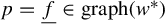 $p=\underline {f} \in \mathrm {graph}(w^*)$
. A plane
$p=\underline {f} \in \mathrm {graph}(w^*)$
. A plane
 $V_p$
is admissible for p if it has the following properties:
$V_p$
is admissible for p if it has the following properties:
-
(1) if
$(\Delta \alpha , \Delta \beta , \Delta b, \Delta \eta _L, \Delta \eta _R) \in V_p$
, then
$|\Delta b| \leq \chi b \|(\Delta \alpha , \Delta \beta , \Delta \eta _L, \Delta \eta _R )\|$
; -
(2)
$V_p$
depends continuously on p with respect to
$d^*_{B_0}$
.


The set of admissible planes for p is denoted by
 $\mathrm {Dual}_p(B_0)$
.
$\mathrm {Dual}_p(B_0)$
.
We let
 $X_1$
denote the space of all admissible plane fields. For clarity of exposition, we will express
$X_1$
denote the space of all admissible plane fields. For clarity of exposition, we will express
 $\underline {f}$
in new coordinates:
$\underline {f}$
in new coordinates:
 $\underline {f} = (b,x)$
, where
$\underline {f} = (b,x)$
, where
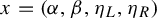 $x=(\alpha , \beta , \eta _L, \eta _R )$
. We use the same notation for a vector
$x=(\alpha , \beta , \eta _L, \eta _R )$
. We use the same notation for a vector
 $\Delta v =(\Delta b, \Delta x)$
, where
$\Delta v =(\Delta b, \Delta x)$
, where
 $\Delta x = (\Delta \alpha , \Delta \beta , \Delta \eta _L, \Delta \eta _R)$
, and although
$\Delta x = (\Delta \alpha , \Delta \beta , \Delta \eta _L, \Delta \eta _R)$
, and although
 $V_{\underline {f}}^*$
is a subspace of
$V_{\underline {f}}^*$
is a subspace of
 $\mathbb {R} \times B_0$
, for the next result we abuse notation and denote the set
$\mathbb {R} \times B_0$
, for the next result we abuse notation and denote the set
 $\{p+v | v \in V_{\underline {f}}^* \}$
also by
$\{p+v | v \in V_{\underline {f}}^* \}$
also by
 $V_{\underline {f}}^*$
.
$V_{\underline {f}}^*$
.
Let
 $p=(b,x)\in w^*$
and define a distance on
$p=(b,x)\in w^*$
and define a distance on
 $\mathrm {Dual}_p(B_0)$
as follows. For any two planes,
$\mathrm {Dual}_p(B_0)$
as follows. For any two planes,
 $V_p,V^{\prime }_p\in \mathrm {Dual}_p(B_0),$
let
$V_p,V^{\prime }_p\in \mathrm {Dual}_p(B_0),$
let
 $\mathcal S$
denote the set of all straight lines
$\mathcal S$
denote the set of all straight lines
 $\gamma $
with direction in
$\gamma $
with direction in
 $C_{r,\delta }.$
Provided that
$C_{r,\delta }.$
Provided that
 $\varepsilon $
is small enough,
$\varepsilon $
is small enough,
 $\gamma $
intersects
$\gamma $
intersects
 $V_p$
at exactly one point, and likewise for
$V_p$
at exactly one point, and likewise for
 $V^{\prime }_p$
. Let
$V^{\prime }_p$
. Let
 $\Delta q_{\gamma }=(\Delta b_{\gamma },\Delta x_{\gamma })=\gamma \cap V_p$
and
$\Delta q_{\gamma }=(\Delta b_{\gamma },\Delta x_{\gamma })=\gamma \cap V_p$
and
 $\Delta q^{\prime }_{\gamma }=(\Delta b^{\prime }_{\gamma },\Delta x^{\prime }_{\gamma })=\gamma \cap V_p'.$
We define
$\Delta q^{\prime }_{\gamma }=(\Delta b^{\prime }_{\gamma },\Delta x^{\prime }_{\gamma })=\gamma \cap V_p'.$
We define
 $$ \begin{align*}d_{1,p}(V_p,V^{\prime}_p)= \sup_{\gamma\in\mathcal S}\frac{|\Delta b_{\gamma}-\Delta b^{\prime}_{\gamma}|}{\min\{|\Delta q_{\gamma}|,|\Delta q^{\prime}_{\gamma}|\}}.\end{align*} $$
When it will not cause confusion, we will omit
 $\gamma $
from the notation. It is not hard to see that
$\gamma $
from the notation. It is not hard to see that
 $d_{1,p}$
is a complete metric. For
$d_{1,p}$
is a complete metric. For
 $V,V'\in X_1,$
we define
$V,V'\in X_1,$
we define
 $$ \begin{align*}d_1(V,V')=\sup_{p\in w^*}d_{1,p}(V_p,V^{\prime}_p).\end{align*} $$
On an absorbing set for renormalization operator, we have that
 $d_1$
is metric and
$d_1$
is metric and
 $(X_1,d_1)$
is a complete metric space. This follows just as in [Reference Martens and Palmisano27, Lemmas 2.29 and 2.30].
$(X_1,d_1)$
is a complete metric space. This follows just as in [Reference Martens and Palmisano27, Lemmas 2.29 and 2.30].
We define the graph transform
 $Q:X_1\to X_1$
by
$Q:X_1\to X_1$
by
 $$ \begin{align*}Q V_{\underline f}=D\underline{\mathcal{R}}_{\underline{\mathcal{R}}\underline f}^{-1}(V_{\underline{\mathcal{R}}\underline f}).\end{align*} $$
Lemma 5.7. Admissible plane fields are invariant under Q. Moreover, Q is contraction on the space
 $(X_1,d_1).$
Proof Let us set
 $p=\underline f.$
To show invariance, assume that
$p=\underline f.$
To show invariance, assume that
 $V_p$
is an admissible plane field, and take
$V_p$
is an admissible plane field, and take
 $(\Delta b,\Delta x)\in QV_p.$
Set
$(\Delta b,\Delta x)\in QV_p.$
Set
 $(\Delta \tilde b,\Delta \tilde x)= D\underline {\mathcal {R}}_p(\Delta b,\Delta x)\in V_{\mathcal R(p)}.$
By Lemma 5.4, we have that
$(\Delta \tilde b,\Delta \tilde x)= D\underline {\mathcal {R}}_p(\Delta b,\Delta x)\in V_{\mathcal R(p)}.$
By Lemma 5.4, we have that
 $\|\Delta b\|\leq K|I'|\|\Delta v\|,$
but now, since
$\|\Delta b\|\leq K|I'|\|\Delta v\|,$
but now, since
 $V_{\underline {\mathcal {R}}(p)}$
is an admissible plane field, we have that
$V_{\underline {\mathcal {R}}(p)}$
is an admissible plane field, we have that
 $K|I'|\|\Delta v\|\leq K_1|I'|\|\Delta x\|,$
where
$K|I'|\|\Delta v\|\leq K_1|I'|\|\Delta x\|,$
where
 $K_1=K_1(K,r,\delta ).$
Furthermore, if
$K_1=K_1(K,r,\delta ).$
Furthermore, if
 $QV_p$
is not continuous in p, then there exists a sequence
$QV_p$
is not continuous in p, then there exists a sequence
 $p_n \rightarrow p$
such that
$p_n \rightarrow p$
such that
 $QV_{p_n}$
does not converge to
$QV_{p_n}$
does not converge to
 $QV_p$
. But now, since
$QV_p$
. But now, since
 $QV_{p_n}$
and
$QV_{p_n}$
and
 $QV_p$
are all codimension-one subspaces, there exists
$QV_p$
are all codimension-one subspaces, there exists
 $\Delta v \in QV_{p}$
such that
$\Delta v \in QV_{p}$
such that
 $\Delta v$
is transverse to
$\Delta v$
is transverse to
 $QV_{p_n}$
for all n sufficiently large. Since
$QV_{p_n}$
for all n sufficiently large. Since
 $V_{\underline {\mathcal {R}}(p)}$
is admissible,
$V_{\underline {\mathcal {R}}(p)}$
is admissible,
 $D \underline {\mathcal R} \Delta v \in V_{\underline {\mathcal {R}}(p)}$
. On the other hand, we can express
$D \underline {\mathcal R} \Delta v \in V_{\underline {\mathcal {R}}(p)}$
. On the other hand, we can express
 $\Delta v=\Delta z'\oplus \Delta z$
with
$\Delta v=\Delta z'\oplus \Delta z$
with
 $\Delta z\in C_{r,\delta }.$
By the invariance of the cone field, we have that
$\Delta z\in C_{r,\delta }.$
By the invariance of the cone field, we have that
 $\Delta \tilde v=\Delta y'\oplus \Delta y$
with
$\Delta \tilde v=\Delta y'\oplus \Delta y$
with
 $\Delta y\in C_{r,\delta }$
. But now,
$\Delta y\in C_{r,\delta }$
. But now,
 $\Delta \tilde v$
is transverse to
$\Delta \tilde v$
is transverse to
 $V_{\underline {\mathcal {R}}(p_n)}$
for all n sufficiently big, which contradicts the admissibility of
$V_{\underline {\mathcal {R}}(p_n)}$
for all n sufficiently big, which contradicts the admissibility of
 $V_p.$
Hence we have that
$V_p.$
Hence we have that
 $QV_p$
depends continuously on p.
$QV_p$
depends continuously on p.
To see that Q is a contraction, take two admissible plane fields
 $V,V'$
, and line
$V,V'$
, and line
 $\gamma \in \mathcal S.$
Define
$\gamma \in \mathcal S.$
Define
 $\Delta q=(\Delta b,\Delta x)\in V$
and
$\Delta q=(\Delta b,\Delta x)\in V$
and
 $\Delta q'=(\Delta b',\Delta x')\in V$
be as in the definition of
$\Delta q'=(\Delta b',\Delta x')\in V$
be as in the definition of
 $d_{1,p}.$
Let
$d_{1,p}.$
Let
 $\Delta \tilde q=(\Delta \tilde b,\Delta \tilde x)=D\underline {\mathcal {R}}_{p}\Delta q$
, and likewise for the objects marked with a prime. Observe that by Lemma 5.4, we have that
$\Delta \tilde q=(\Delta \tilde b,\Delta \tilde x)=D\underline {\mathcal {R}}_{p}\Delta q$
, and likewise for the objects marked with a prime. Observe that by Lemma 5.4, we have that
 $\|\Delta q\|\geq ({1}/{C_1})\tilde \|\Delta \tilde q\|,$
and that
$\|\Delta q\|\geq ({1}/{C_1})\tilde \|\Delta \tilde q\|,$
and that
 $|\Delta b|\leq C_2|I'\|\Delta \tilde b|$
. So
$|\Delta b|\leq C_2|I'\|\Delta \tilde b|$
. So
 $$ \begin{align*}\frac{|\Delta b-\Delta b'|}{\min\{\|\Delta q\|,\|\Delta q'\|\}}\leq C|I'|\frac{|\Delta\tilde b-\Delta\tilde b'|}{\min\{\|\Delta\tilde v\|,\|\Delta\tilde v\|\}}\leq \frac{1}{2}d_{1,\underline{\mathcal{R}}(p)}(V_{\underline{\mathcal{R}}({p)}}, V_{\underline{\mathcal{R}}(p)}').\end{align*} $$
Thus,
 $$ \begin{align*}d_{1}(QV,QV')\leq\tfrac{1}{2} d_1(V,V').\\[-32pt]\end{align*} $$
Thus we have that there is an admissible plane field
 $V^*(\underline f),$
which is an invariant plane field under Q.
$V^*(\underline f),$
which is an invariant plane field under Q.
Now we conclude the proof of the proposition. We will show that for each
 $\underline f\in \mathrm {graph}(w^*)$
,
$\underline f\in \mathrm {graph}(w^*)$
,
 $V^*(\underline f)=T_{\underline f}(\mathrm {graph}(w^*)).$
Let
 $p \in \mathrm {graph}(w^*)$
and take an almost horizontal curve
$p \in \mathrm {graph}(w^*)$
and take an almost horizontal curve
 $\gamma $
close enough to p such that
$\gamma $
close enough to p such that
 $\gamma \cap \mathrm {graph}(w^*) = q =\{ p+ \Delta q = p+ (\Delta \alpha , \Delta \beta , \Delta b, \Delta \eta _L, \Delta \eta _R) \}$
and
$\gamma \cap \mathrm {graph}(w^*) = q =\{ p+ \Delta q = p+ (\Delta \alpha , \Delta \beta , \Delta b, \Delta \eta _L, \Delta \eta _R) \}$
and
 $\gamma \cap V_{\underline {f}}^* = q'= \{ p+ \Delta q' = p+ (\Delta \alpha ', \Delta \beta ', \Delta b', \Delta \eta _L', \Delta \eta _R') \}$
. We define
$\gamma \cap V_{\underline {f}}^* = q'= \{ p+ \Delta q' = p+ (\Delta \alpha ', \Delta \beta ', \Delta b', \Delta \eta _L', \Delta \eta _R') \}$
. We define
 $$ \begin{align*} A = \sup_{p} \limsup_{\gamma \rightarrow p} \frac{|\Delta b - \Delta b'|}{|\Delta v|}. \end{align*} $$
A straightforward calculation shows that at deep renormalization levels, we have that
 $A \leq 1$
, cf. [Reference Martens and Palmisano27, Lemma 2.34].
$A \leq 1$
, cf. [Reference Martens and Palmisano27, Lemma 2.34].

Figure 3 Notation for the proof of Proposition 5.5.
Proof of Proposition 5.5 We show that at a deep level of renormalization, each point
 $\underline {f} \in \mathrm {graph(w^*)}$
has a tangent plane
$\underline {f} \in \mathrm {graph(w^*)}$
has a tangent plane
 $T_{\underline {f}}w^* = V_{\underline {f}}^*$
. To get this result, it is enough to show that
$T_{\underline {f}}w^* = V_{\underline {f}}^*$
. To get this result, it is enough to show that
 $A=0$
. We use the notation from the definition of A and we introduce the following notation:
$A=0$
. We use the notation from the definition of A and we introduce the following notation:
 $$ \begin{align*} \begin{array}{@{}r@{}c@{\,}l} \underline{\mathcal{R}}(\underline{f})& \,=\, & (\tilde{b}, \tilde{x}), \\[4pt] \underline{\mathcal{R}} (\gamma) \cap \mathrm{graph}(w^*) & \,=\, & \tilde{q} = \underline{\mathcal{R}}(q) = \underline{\mathcal{R}}(\underline{f}) + \Delta \tilde{q} = \underline{\mathcal{R}}(\underline{f}) + ( \Delta \tilde{b}, \Delta \tilde{x} ), \\[4pt] \underline{\mathcal{R}}(\gamma) \cap V_{\underline{\mathcal{R}}(\underline{f})}^{*} & \,=\, & z = \underline{\mathcal{R}}(\underline{f})+ \Delta z, \\[4pt] \underline{\mathcal{R}}(q') & \,=\, & \tilde{q}'= \underline{\mathcal{R}}(\underline{f})+ \Delta \tilde{q}' = \underline{\mathcal{R}}(\underline{f})+ ( \Delta \tilde{b}', \Delta \tilde{x}'), \\[4pt] z-\tilde{q} & \,=\, & ( \Delta h_1, \Delta u ), \\[4pt] \tilde{q}' - z & \,=\, & ( \Delta h, \Delta u_1 ), \\[4pt] \Delta \tilde{q}' & \,=\, & D \underline{\mathcal{R}}_{\underline{f}} ( \Delta q') + \Delta \epsilon, \\[4pt] D \underline{\mathcal{R}}_{\underline{f}} ( \Delta q') - \Delta z & \,=\, & ( \Delta h_2, \Delta u_2 ). \end{array} \end{align*} $$
For almost horizontal curves
 $\gamma $
such that
$\gamma $
such that
 $\gamma \cap \mathrm {graph}(w^*)$
is close enough to p, we get
$\gamma \cap \mathrm {graph}(w^*)$
is close enough to p, we get
 $$ \begin{align} |\Delta \epsilon | = o ( |\Delta q'| ), \end{align} $$
and
 $$ \begin{align} \| \Delta u_2 - \Delta u_1\| \leq |\Delta \epsilon|. \end{align} $$
Since
 $\underline {\mathcal {R}}$
has strong expansion on the b direction, and using the differentiability of
$\underline {\mathcal {R}}$
has strong expansion on the b direction, and using the differentiability of
 $\underline {\mathcal {R}}$
, we get
$\underline {\mathcal {R}}$
, we get
 $$ \begin{align} |\Delta h_1|+|\Delta h| \geq \displaystyle \frac{1}{|I'|} \cdot |\Delta b - \Delta b'|. \end{align} $$
As
 $(\Delta h_2, \Delta u_2) \in V_{\underline {f}}^*$
and
$(\Delta h_2, \Delta u_2) \in V_{\underline {f}}^*$
and
 $V_{\underline {f}}^*$
is an admissible plane, we get
$V_{\underline {f}}^*$
is an admissible plane, we get
 $$ \begin{align} |\Delta h_2| \leq 2 \chi \tilde{b} \|\Delta u_2 \|. \end{align} $$
Since
 $q'-q = (\Delta b'- \Delta b, \Delta x'- \Delta x)$
is a tangent vector to the curve
$q'-q = (\Delta b'- \Delta b, \Delta x'- \Delta x)$
is a tangent vector to the curve
 $\gamma $
, it is inside the cone
$\gamma $
, it is inside the cone
 $C_{r, \delta }$
, and then we get
$C_{r, \delta }$
, and then we get
 $$ \begin{align} \|\Delta x'- \Delta x \| < |\Delta b'- \Delta b|. \end{align} $$
As
 $(\Delta h, \Delta u_1)$
is a tangent vector to the curve
$(\Delta h, \Delta u_1)$
is a tangent vector to the curve
 $\underline {\mathcal {R}}_{\underline {f}}(\gamma )$
, by the same reason as before, we get
$\underline {\mathcal {R}}_{\underline {f}}(\gamma )$
, by the same reason as before, we get
 $$ \begin{align} \|\Delta u_1 \| < |\Delta h|. \end{align} $$
By (5.7), (5.5), and (5.9), we have
 $$ \begin{align*} |\Delta h | &\leq |\Delta \epsilon| + |\Delta h_2| \leq |\Delta \epsilon| + 2 \chi \tilde{b} \| \Delta u_2\| \\ & \leq |\Delta \epsilon| + 2 \chi \tilde{b} \| \Delta u_2-\Delta u_1\| + 2 \chi \tilde{b} \|\Delta u_1\|\\ & \leq |\Delta \epsilon| + 2 \chi \tilde{b} |\Delta \epsilon|+ 2 \chi \tilde{b} |\Delta h|. \end{align*} $$
Hence, when we are in a deep level of renormalization, we have
 $$ \begin{align} |\Delta h| \leq 2 |\Delta \epsilon|. \end{align} $$
Since
 $$ \begin{align*} |\Delta q'| \leq |\Delta q| + \|q'-q\| = |\Delta q| + \|\Delta x' - \Delta x\| + |\Delta b'- \Delta b|, \end{align*} $$
from (5.4) and (5.8), we obtain
 $$ \begin{align*} |\Delta \epsilon| = o ( |\Delta q| + 2 |\Delta b'- \Delta b| ) = o ( |\Delta q| (1+2A ) ). \end{align*} $$
Hence
 $$ \begin{align} |\Delta \epsilon| = o ( |\Delta q| ). \end{align} $$
From this and using Lemma 5.4, we have
 $$ \begin{align*} \displaystyle \frac{|\Delta b - \Delta b'|}{|\Delta v|} & \leq \displaystyle \frac{C_1 \cdot |I'| \cdot ( |\Delta h_1|+|\Delta h|) }{|\Delta v|} = C_1 \cdot |I'| \cdot \frac{|\Delta h_1| }{|\Delta v|} + C_1 \cdot |I'| \cdot \frac{|\Delta h| }{|\Delta v|} \\ & = \displaystyle C_1 \cdot |I'| \cdot \frac{|\Delta \tilde{v}|}{|\Delta v|} \cdot \frac{|\Delta h_1| }{|\Delta \tilde{v}|} + C_1 \cdot |I'| \cdot \frac{|\Delta h| }{|\Delta v|} \\ & \leq C_2 \cdot |I'| \cdot \displaystyle \frac{|\Delta h_1|}{|\Delta \tilde{v}|} + o(1), \end{align*} $$
for a constant
 $C_2>0$
. Hence, we obtain
$C_2>0$
. Hence, we obtain
 $$ \begin{align*} \displaystyle \limsup_{\gamma \rightarrow p} \frac{|\Delta b - \Delta b'|}{|\Delta v|} \leq O(|I'|) A. \end{align*} $$
Since
 $|I'|$
goes to zero when the level of renormalization goes to infinity, we conclude that
$|I'|$
goes to zero when the level of renormalization goes to infinity, we conclude that
 $A=0$
, as desired.
$A=0$
, as desired.
Thus we have proved that there is an absorbing set,
 $B_0,$
for the renormalization operator within which the topological conjugacy class of
$B_0,$
for the renormalization operator within which the topological conjugacy class of
 $\underline f$
is a
$\underline f$
is a
 $\mathcal C^1$
manifold. It remains to prove that it is globally
$\mathcal C^1$
manifold. It remains to prove that it is globally
 $\mathcal C^1$
.
$\mathcal C^1$
.
By [Reference Gouveia and Colli17, Lemma 5.1], each infinitely renormalizable gap mapping
 $f_0=(f_{R},f_L,b_0)$
can be included in a family
$f_0=(f_{R},f_L,b_0)$
can be included in a family
 $f_t,$
for
$f_t,$
for
 $t\in (-\varepsilon _0,\varepsilon _0)$
of gap mappings, which is transverse to the topological conjugacy class of
$t\in (-\varepsilon _0,\varepsilon _0)$
of gap mappings, which is transverse to the topological conjugacy class of
 $f_0.$
The construction of this family is given by varying the b parameter in a small neighborhood about
$f_0.$
The construction of this family is given by varying the b parameter in a small neighborhood about
 $b_0$
, and observing that the boundary points of the principal gaps at each renormalization level are strictly increasing functions in b. Thus, we have that the transversality of this family is preserved under renormalization. Let
$b_0$
, and observing that the boundary points of the principal gaps at each renormalization level are strictly increasing functions in b. Thus, we have that the transversality of this family is preserved under renormalization. Let
 $\Delta f$
denote a vector tangent to the family
$\Delta f$
denote a vector tangent to the family
 $f_t$
at
$f_t$
at
 $f.$
We have the following.
$f.$
We have the following.
Lemma 5.8. Let
 $n_0\in \mathbb N$
be so that
$n_0\in \mathbb N$
be so that
 $\underline {\mathcal {R}}^{n_0}( \underline f)\in B_0.$
Then
$\underline {\mathcal {R}}^{n_0}( \underline f)\in B_0.$
Then
 $D\underline {\mathcal {R}}^{n_0}(\Delta f)\notin T_{\underline {\mathcal {R}}^{n_0} f} \mathrm {graph}(w^*),$
where
$D\underline {\mathcal {R}}^{n_0}(\Delta f)\notin T_{\underline {\mathcal {R}}^{n_0} f} \mathrm {graph}(w^*),$
where
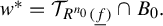 $w^*=\mathcal T_{R^{n_0}(\underline f)}\cap B_0.$
Using this lemma, we can argue as in the proof of [Reference de Faria, de Melo and Pinto10, Theorem 9.1] to conclude the proof Theorem 1.1.
Theorem 5.9.
 $\mathcal T_f\subset \mathcal D^4$
is a
$\mathcal T_f\subset \mathcal D^4$
is a
 $\mathcal C^1$
manifold.
$\mathcal C^1$
manifold.
Note that the application of the implicit function theorem in the proof is why we lose one degree of differentiability.
Acknowledgements
This work has been partially supported by ERC AdG grant no 339523 RGDD; EU Marie-Curie IRSES Brazilian–European partnership in Dynamical Systems (FP7-PEOPLE-2012-IRSES 318999 BREUDS); FAPESP grants 2017/25955-4 and 2013/24541-0, and CAPES. The authors would like to Liviana Palmisano for some helpful comments about [Reference Martens and Palmisano27]. They also thank Sebastian van Strien for his encouragement and several helpful conversations.


 Open access