


1. Introduction
Since the seminal contribution of Pigou (Reference Pigou1920), it has been known that market failures caused by negative pollution externalities can be corrected by environmental policies. Climate change has been called the ‘greatest market failure ever’ (Stern, Reference Stern2007). The method to derive policy conclusions thus appears to be standard; the mere fact that greenhouse gas emissions and their economic impacts are large should not have an impact on the basic concept. Yet, economic climate models and associated policy recommendations have suffered from different problems, notably the modelling of climate damages, the incomplete characterization of growth, or the lacking specifications of resource markets. Recently, this strand of research has even been harshly criticized (see Pindyck, Reference Pindyck2013; Farmer et al., Reference Farmer, Hepburn, Mealy and Teytelboym2015; Stern, Reference Stern2016). The reason for the critique lies in the difficulty in properly integrating climate change in economic models, in particular with respect to the interdependence between the ecological and the economic system, the long-run character of climate change, the link of emissions to natural resource depletion, and the nature and size of climate damages.
These issues pose serious challenges for developing a theory framework which includes sufficient precision to be useful while remaining clearly arranged to be intuitive. Specifically, one has to be careful when embedding ecological relationships related to climate change in an economic framework; model assumptions have to be in accordance with the results from natural sciences.Footnote 1 Moreover, climate policy assessment models should reflect the state of the art in resource economics and dynamic macroeconomic modelling. As global warming affects the world economy for a very long time, economic development and its interactions with the resource stock in the ground and the pollution stock in the atmosphere are crucial and should be determined endogenously; a purely static analysis is not applicable in climate economics (Bretschger, Reference Bretschger2017).
Recent papers have addressed important points of the critique by pushing the frontiers in economic theory, refining functional relationships and improving numerical calibration.Footnote 2 But contributions have become very technical and quite specialized; for a broader audience it is often difficult to get an overview. The same holds true for quantitative models, for which Weitzman (Reference Weitzman2010) states: ‘Because the climate change problem is so complex, there is frequent reliance on numerical computer simulations. These can be indispensable, but sometimes they do not provide a simple intuition for the processes they are modelling’. What is lacking in the literature is an illustrative general model showing the basic theoretical relationships of an economic climate model, including the most recent advances, in an intuitive manner. Such an approach can be used for educational activities and for communication, mainly within the scientific community but also with policy makers and the broader public. It can be especially useful in highlighting how different model assumptions affect the policy conclusions and how different policies are affecting the economy.
The present paper aims to fill this gap. We develop a simple flexible framework that integrates the economic approach to climate change labelled the ‘Basic Climate Economic model’; henceforth the BCE model. In order to be useful for communication and broad knowledge diffusion, the paper starts by working with figures and verbal explanations. This should underline the basic reasoning in climate economics, show the different model parts in an intuitive form, and reveal the specific effects of different model assumptions. The model elements we are using concern natural resource stock depletion, pollution stock accumulation, pollution externalities in the form of climate damage functions, capital accumulation, and endogenous growth. Policies will affect one or multiple elements and have an effect on economic development. Also we will show the main differences between the BCE model and existing economic climate models that have drawn attention in the literature, namely the DICE model (Nordhaus, Reference Nordhaus2017) and the model of Golosov et al. (Reference Golosov, Hassler, Krusell and Tsyvinski2014).
The remainder of the paper is organized as follows. Section 2 contains a graphical model analysis of the theory and of policy impacts. In section 3 we provide the theoretical foundation for the graphical approach, presenting analytical solutions and quantitative applications to replicate the figures of the previous section. Section 4 presents a comparison of our model to existing literature and section 5 concludes.
2. Graphical approach
This section develops the BCE model step by step, providing basic intuition about the different model mechanisms and their economic impact. Here we use curves and figures which will be mathematically derived in the next section of the paper. We start with a theory part and subsequently add policy effects.
2.1. Climate economics theory
The climate problem originates from the release of greenhouse gases into the atmosphere. The dominant share of these gases are carbon emissions which stem from burning fossil fuels. Stocks of these fuels are ultimately bounded so that an economic analysis should be based on the theory of optimal exhaustible resource depletion (Hotelling, Reference Hotelling1931). For the sake of clarity we abstract here from new resource discoveries and extraction costs.Footnote 3 When resources are continuously extracted, which we assume, the stock of remaining resources decreases over time. In figure 1, resource stock S starts at S 0 in time t = 0 and decreases in time t along the curved line.

Figure 1. Resource stock depletion over time.
The curvature of stock development as shown in figure 1 is based on the basic result of Hotelling (Reference Hotelling1931) which says that prices of exhaustible resources are driven by the resource rent, reflecting increasing resource scarcity over time. In standard resource models, the scarcity effect induces decreasing resource use over time so that the negative slope of the S(t) function becomes smaller with growing t (Dasgupta and Heal, Reference Dasgupta and Heal1974); see the next section for a more formal derivation.Footnote 4
The stock of carbon in the atmosphere depends on total resource use in a linear way, with a fixed coefficient representing the carbon content of used fossil fuels. Natural decay of the pollution stock has been included in various economic models with a constant depreciation rate, which is convenient. In reality, however, the decay of greenhouse gases is a very complex and long-lasting process. Part of the emission stock disappears relatively quickly while the largest share stays in the atmosphere for several hundred years.Footnote 5 Hence it is preferable to abstract from decay and to focus on a linear relationship between extracted resource stock (S 0 − S) and total pollution stock P. In figure 2 we have flipped the figure for resource stock of figure 1 around the horizontal axis and included pollution stock in the lower left quadrant measuring P from right to left. The economy starts at t = 0 and continuously depletes the resource stock which simultaneously raises pollution along the P(S) line. Since S is a function of time, this line implies the time evolution of pollution stock, i.e., P t = P(S t). As shown in the figure, in times 1,2 the pollution stocks amount to P 1 and P 2 > P 1; as the stock of resources gets depleted, pollution accumulates.
Figure 2. The relationship between pollution and resource stocks.
The next step concerns the impact of climate change, expressed in temperature, on the economy. Following recent climate physics, the relationship between pollution stock and temperature is almost linear (Hassler et al., Reference Hassler, Krusell, Smith, Taylor and Uhlig2016; Brock and Xepapadeas, Reference Brock and Xepapadeas2017; Dietz and Venmans, Reference Dietz and Venmans2017).Footnote 6 Hence we do not need to introduce a separate variable for temperature but can directly proceed with the (appropriately scaled) pollution variable. The shape and the parameterization of the function relating pollution stock to economic damages are major points of concern and dispute; see Dietz and Stern (Reference Dietz and Stern2015). To show the impacts in the model, we need to further specify the kind of economic damages. Recent weather and climate disasters like hurricanes and landslides have harmed the affected regions most by destroying significant parts of the capital stocks, especially physical capital in the form of infrastructure, buildings, roads, etc.Footnote 7 Correspondingly, in our model, part of the capital stock will be destroyed (i.e., depreciated) in each point in time due to climate change. Figure 3 shows the function for the damage rate D, expressed as a percentage of capital stock, and as a function of pollution stock P. The function is bounded between 0 and 1 and increasing in P; in principle it can be assumed convex, concave, or convex-concave (sigmoid), as shown in the figure.Footnote 8
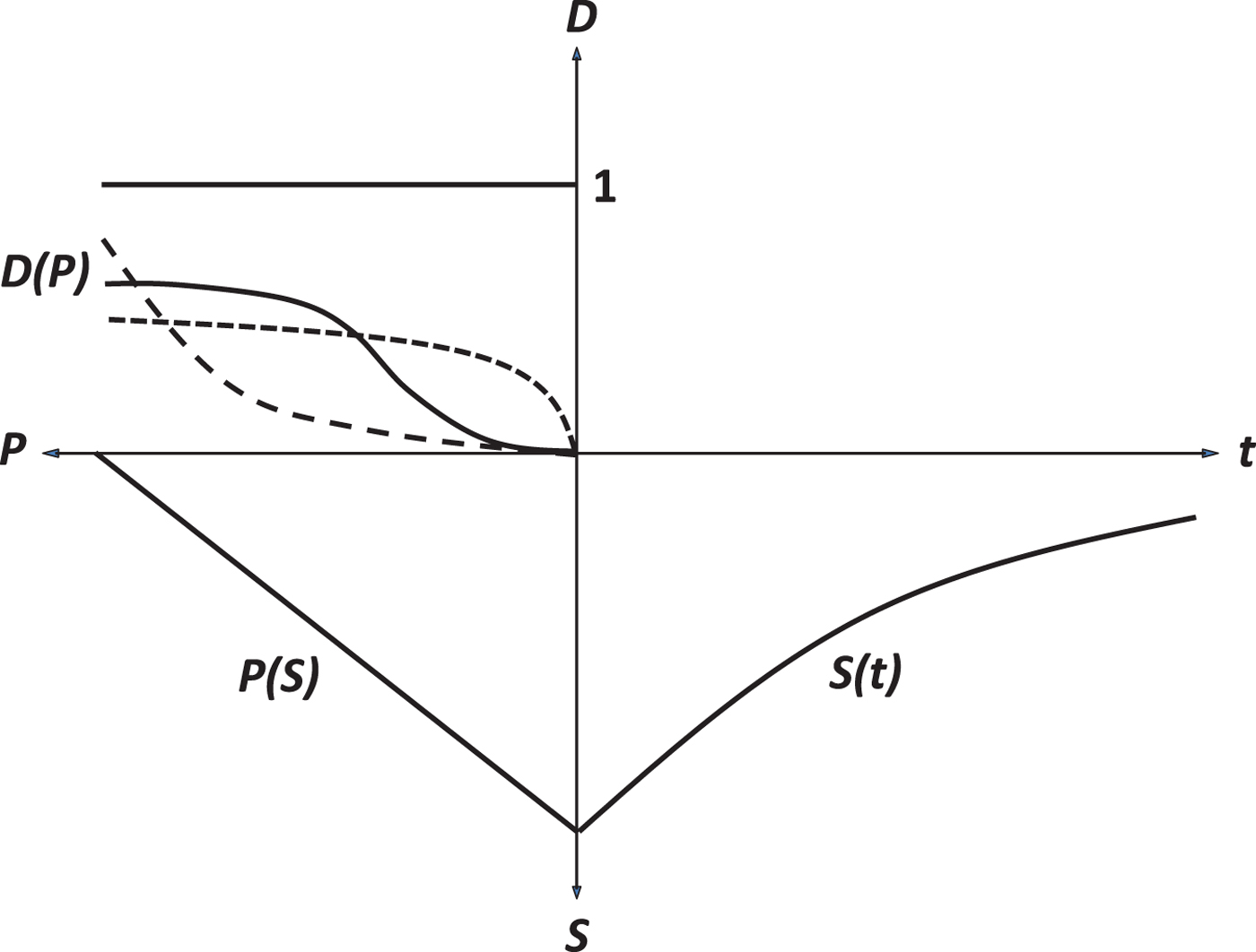
Figure 3. Different forms of the damage function D(P).
We are now ready to represent climate damages as a function of time in the first quadrant on the upper right; see figure 4 for the example of the convex-concave damage function. Each line linking the different functions translates the extracted resource stock to pollution and damages at a certain point in time. We see from the figure that the line in the first quadrant is shaped by the form of the damage function while its position depends on the size of available resource stock and pollution intensity of resource use.
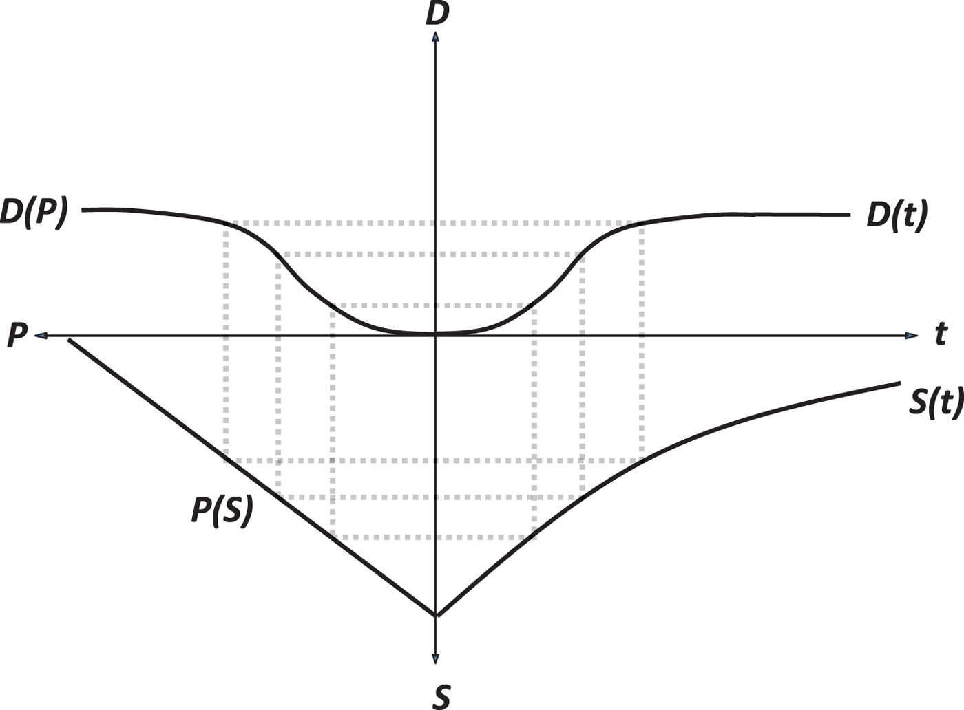
Figure 4. The convex-concave (sigmoid) damage function D(P).
To derive the impact of climate change on economic growth, climate-induced capital depreciation has to be confronted with the other dynamic elements stemming from capital accumulation. It is known from basic macroeconomics that the optimal consumption growth rate depends on the utility function of households, on marginal capital productivity, and on capital depreciation. The famous ‘Keynes-Ramsey’ rule widely used in growth theory says that consumption growth is positively affected by capital productivity, and negatively affected by discounting and the capital depreciation rate, which in our case is exacerbated by climate change. We can then represent the growth rate of consumption ($\hat {C}$ ) by the difference between the capital productivity effect, which we label Ω, and the sum of the discounting effect (Δ), and the capital depreciation effect due to natural depreciation but also climate change (Λ), i.e., growth is given by $\hat {C}= \Omega -\Delta -\Lambda$
 . As usual, we take the utility discount rate as given. Here we use our damage function to display the effect of climate-induced capital depreciation graphically.
Figure 5 shows the consumption growth rate for a convex-concave damage function as the difference between productivity net of discounting (Ω − Δ) and climate-induced depreciation (Λ). With given Ω and Δ, it is immediately seen that the growth rate of the economy depends on capital damages Λ, and may be positive or negative depending on the model parameters. As pollution accumulates and climate deteriorates, so does economic growth, which reaches its steady state when pollution reaches its maximum level (P max). The figure shows the case of a falling but positive consumption growth rate, which is likely for the world economy but may be unrealistic for a climate vulnerable region such as a small island state for which the Λ line might cross the Ω − Δ line from below, thus implying negative growth.Footnote 9

Figure 5. Effects of productivity (Ω), discounting (Δ), and depreciation (Λ) on growth.
2.2. Changing modelling conditions
The graphical model approach can now be used to discuss various core parts of the model and to show their impacts on economic development. Assuming the same shape of the damage function but a higher damage intensity of each pollution unit lowers the growth rate as shown in figure 6(a), where long-run growth becomes zero after a transition period; it may as well remain positive or become negative, this is a matter of appropriate calibration. The case of a purely convex damage function is shown in figure 6(b). In the example, the long-run growth rate remains positive due to decreasing resource use over time, but this is just one of the possible cases; the growth rate may also turn negative depending on the convexity of the damage function.Footnote 10 The case of a delay in pollution accumulation is given in figure 6(c), where pollution has a relatively lower impact at the time of emission but an additional impact at a later stage because of the time lag between resource extraction and damages.Footnote 11 Finally, changing capital productivity over time due to a sectoral change of the economy is represented in figure 6(d).Footnote 12 In the favorable case of increasing capital productivity over time, as shown in the figure, economic growth is supported by structural change so that adverse climate effects can be alleviated; when sectoral change reduces capital productivity, both the productivity and the climate effect are harming the growth rate in the economy.
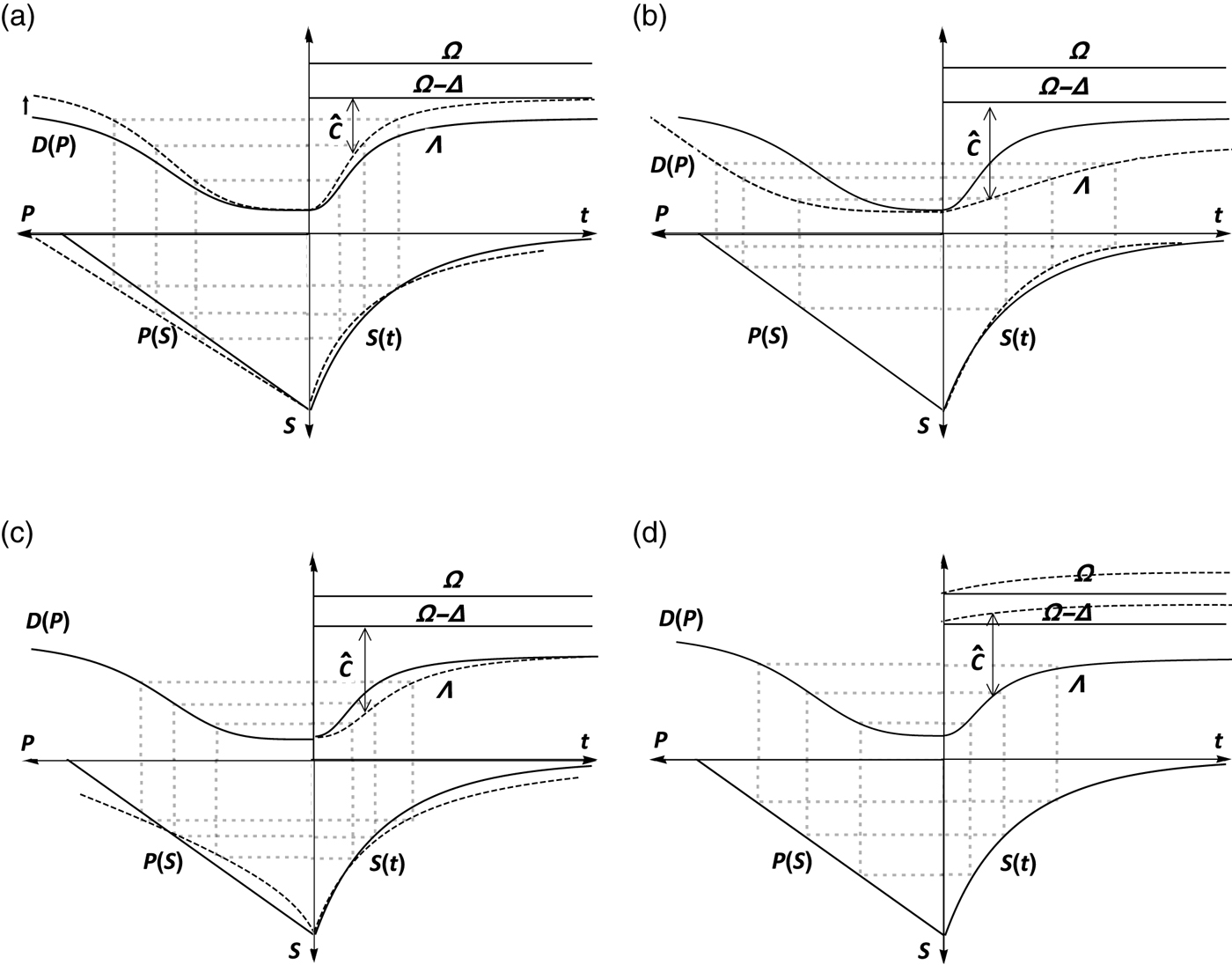
Figure 6. Changing model's parameters (solid – baseline model, dashed – new parameters). (a) Increasing pollution intensity (b) Convex damages (c) Lags in pollution accumulation (d) Increasing capital productivity.
2.3. Climate policies
The graphical model approach can be conveniently used to show the effects of different climate policies. Real-life policy-making is rarely optimal and, therefore, the policies examined are not optimal policies, i.e. they do not necessarily align the decentralized equilibrium with the social planner solution. The most widely studied policy is the use of carbon taxes, the effects of which are shown in figure 7(a). Carbon taxation delays polluting resource extraction, and thus pollution accumulation. It follows that economic growth is higher all along the transition to the steady state, which is unaffected by the policy.Footnote 13 It is an important feature of the model setup with costless extraction of exhaustible resources that taxation of resource use shifts the resource extraction profiles in time but never induces resource owners to leave resources unutilized in the ground. This would, however, exactly be needed for an effective climate policy, because climate physics predicts that the extraction of all fossil resources will cause very high damages, irrespective of the extraction profile; see Meinshausen et al. (Reference Meinshausen, Meinshausen, Hare, Raper, Frieler, Knutti, Frame and Allen2009) and McGlade and Ekins (Reference McGlade and Ekins2015). One way employed in the literature is the inclusion of increasing extraction costs and the costly development of clean backstop technologies as perfect substitutes to the incumbent resource, as in van der Ploeg and Withagen (Reference van der Ploeg and Withagen2012). Here we take a different stand and examine the case of directly decommissioning part of the polluting resource stock as a policy option.
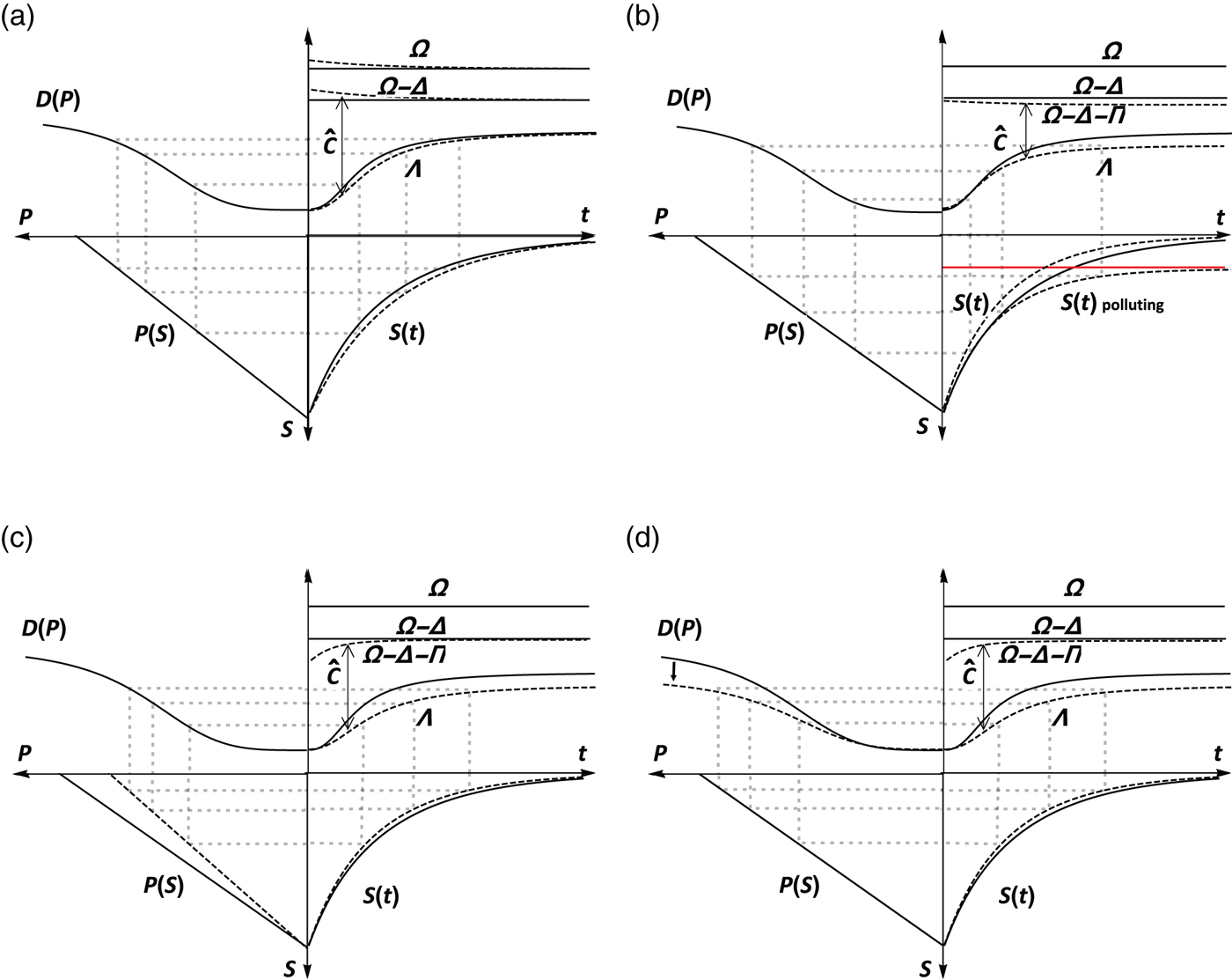
Figure 7. Effects of different policies (solid – baseline model, dashed – effects of policy). (a) Carbon taxation (b) Decommissioning (c) CCS (d) Adaptation.
Figure 7(b) shows as an example the case of decommissioning part of the available stock of fossil fuels each year; the technical section shows how the policy is implemented in the model. With S(t) we denote the available resource stock in time t, after the policy has been implemented, which naturally declines to zero over time. Variable S(t)polluting reads as the effective stock of polluting resources, which is bounded by policy. The difference between these two curves is the amount of resources decommissioned up to time t. Total decommissioning is visualized by the red limitations to resource stock which is available for the economy. The stock measured as a difference between the red line and the origin is not available for commercial use and is thus not augmenting the pollution stock. Factor Π shows the negative effect of policy on the growth rate of consumption: intuitively, since decommissioning reduces the profitability of fossil assets, this should be reflected in the rate of economic growth. In the end, if the benefit of reduced emissions (lower Λ line) outweighs the cost of the policy (factor Π), economic growth is promoted.
If a certain part of the capital stock is used for abatement activities, we obtain two effects in the model. First, because abatement is costly, we have to reduce capital productivity by a policy factor Π, which lowers the growth potential of the economy. For the second effect there are two cases. When each extracted resource unit has a lower impact on pollution stock P, as in the case of carbon capture and sequestration (CCS), the straight line in the lower left quadrant is rotated clockwise, as shown in figure 7(c). As a consequence, there is a lower (negative) impact of resource extraction on capital depreciation such that the growth rate is affected positively. When we look at adaptation to climate change, i.e., the building of dams or other specific protection, the pollution stock has a lower impact on capital depreciation as shown in the upper left quadrant of figure 7(d), which again affects economic growth positively. The total effect of the policies is given by adding the two separate impacts.
Finally, it would be instructive to see how optimal policy would look like in our setup. The social planner solution would most closely resemble the case of resource taxation, where the tax rate is set at the social cost of carbon.Footnote 14 Resource extraction would be stretched further in time (flatter extraction profile) and so would pollution accumulation. This would also induce a flatter growth profile towards the steady state, i.e., higher growth at all times during transition in comparison to the no-policy case.
3. Formal analysis
This section formally presents the theoretical foundation of the BCE model. The model builds on the two-sector AK model of endogenous growth introduced by Rebelo (Reference Rebelo1991), as modified by Bretschger and Karydas (Reference Bretschger and Karydas2018) to include polluting non-renewable resources as a productive input, and pollution-induced damages to the capital stock.Footnote 15 In comparison to the aforementioned contribution, here we abstract from lags in pollution accumulation, we include a more rigorous representation of the damage function (sigmoid instead of linear), and we examine a much larger set of climate policy alternatives. We will first present the basic model and subsequently the alterations needed to get the results for each policy option. Our analysis focuses on a closed economy in continuous time.
3.1. Theory
Climate change and damages
Before we describe the macroeconomic environment, we present our assumptions on the climate system, on pollution, and how it feeds back in the economy by destroying stocks of available capital. Polluting non-renewable resources are used as inputs in production. Let S t denote the stock of non-renewable resources available in time t and R t the resource extraction. Extracting and burning fossil fuels in time t depletes the resource stock and simultaneously adds to the existing stock of pollution P t according to:

and

with ϕ > 0 the pollution intensity of the non-renewable resource. Resource extraction is decreasing over time leading to a decreasing time profile for the resource stock as in figure 1. Combining the above two equations leads to a linear relationship between the stock of pollution and the stock of non-renewable resources; the P(S) line in figure 2:Footnote 16

As the stock of non-renewable resources gets depleted, pollution increases. When the whole stock is depleted, pollution gets its maximum value P max = P 0 + ϕ S 0. We use pollution stock as a measure of climate change. The linear relationship of equation (2), between the change in the variable responsible for climate change and greenhouse gas emissions, is well founded in the literature.Footnote 17 Natural disasters caused by man-made pollution are increasingly harming economic activity by destroying available stocks of capital. In our model, climate change damages are measured as a percentage of the available stock of capital in each period. We will assume that pollution feeds back in the economy through a sigmoid damage function D(P), according to:
with δ0 ∈ [0, 1], the natural depreciation of the capital stock, δ1 ∈ [0, 1 − δ0], δ2 > 0, scaling parameters, and η ≥ 1 a convexity parameter. A similar functional form is used in the latest DICE-2016R model but there damages reduce aggregate productivity and not capital stock; see Nordhaus (Reference Nordhaus2017). With this damage function we make sure that damages as a percentage of the stock of capital are bounded between 0 and 1, while at the same time we can calibrate it such that the mapping between pollution and damages is convex for the relevant range of available polluting resources, as typically advocated in the literature (e.g., Golosov et al., Reference Golosov, Hassler, Krusell and Tsyvinski2014).Footnote 18
Macroeconomic environment
There are two financial assets owned by households: a stock of polluting non-renewable resources S, and capital K. There are also two economic sectors: the manufacturing sector that produces goods readily available for consumption, and the corporate sector that provides goods and services for investments that augment the stock of capital.
In order to produce the consumption good Y, the manufacturing sector combines a part of physical capital K Y with non-renewable resources R in a Cobb-Douglas fashion:

Parameters $\alpha \in \lbrack 0,1]$ and A>0 represent the capital expenditure share and the productivity of the manufacturing sector, respectively. According to the Cobb-Douglas specification of (5), we assume that polluting non-renewable resources are essential inputs in the production of the consumer good. In fact, empirical evidence is inconclusive about whether the elasticity of substitution between capital and polluting energy resources is above unity or not. Van der Werf (Reference van der Werf2008) uses industry-level data from 12 OECD countries and consistently finds elasticities of substitution between energy and other inputs which are smaller than unity. Hassler et al. (Reference Hassler, Krusell and Olovsson2015) suggest very low elasticities of substitution between capital and energy in the short run, but high elasticities in the long run, while Papageorgiou et al. (Reference Papageorgiou, Saam and Schulte2017) find elasticities above unity.
Before we draw, however, any pessimistic conclusions about future economic development, note that in our framework there are two ways of substituting towards clean resources and cleaning up the pollution from the dirty resources at finite cost. First, capital K is clean and is assumed to include renewable energy capital such as solar panels, dams and windmills; the availability of renewable energies clearly requires long-run capital investments. Second, we explicitly analyze the policy of cleaning up by looking at Carbon Capture and Sequestration (CCS) as already presented in the graphical part of the paper. With CCS we have directly the possibility to clean up the pollution stock at finite costs.
In turn, the corporate sector, responsible for providing the investment good I, has a linear technology in physical capital K I:

with B>0 a productivity parameter. The pollution stock is responsible for climate change and damages to the existing stock of capital through function D(P) defined in (4).Footnote 19 Capital accumulation reads:

Finally, households receive rents from physical capital and non-renewable resources and balance their income with expenditure on the consumption good C, and on the investment good H, the latter being the equivalent of savings in the present economy. In equilibrium, households demand the total consumption and investment goods, i.e., C = Y and H = I respectively, while capital is exactly shared between the manufacturing and the investment sector, i.e., K Y + K I = K; GDP in this economy reads p YY + p II, with p Y, p I the prices of the consumption and the investment good, respectively. Let us now proceed by describing the market economy and the equilibrium.
Firms
Let the consumption good Y be the numeraire, i.e., p Y = 1. Firms in both sectors maximize instantaneous profits according to:

with p K the rental price of capital, p R the price of non-renewable resources, and p I the price of the investment good, i.e., the price of investment in new forms of capital. Let us define with ϵ ≡ K Y/K the share of total available capital employed by the manufacturing sector. With (5) and (6), this maximization gives the demand curves for non-renewable resources and capital in the two sectors:

The last two equations imply a no-arbitrage condition for the use of capital between sectors: employing the marginal unit of capital in the two sectors should yield the same return.
Households
Households allocate their rental income from physical capital and non-renewable resources between expenditure on consumption C and on additional capital formation H. Let T represent generic non-distorting lump-sum transfers. Then, the income balance reads:

Expenditure on capital formation adds to the existing stock of capital according to:

although agents do not internalize damages to capital accumulation through higher levels of pollution. Total wealth reads W = p I K + p R S. Time-differentiation of total wealth using (1), (10), (11), and the fact that p K = p I B from (9), leads to the household's dynamic budget constraint, according to:

with θ ≡ p R S/W, the share of the individual's resource wealth in the total assets; hats denote growth rates, i.e., $\hat {p}=\dot {p}/p$ . Finally, the representative household chooses the time path of consumption C and asset allocation θ in order to maximize lifetime utility:

subject to the budget constraint (12); ρ > 0 is the intergenerational discount rate. We will assume throughout that households have constant relative risk aversion (CRRA) preferences according to U(C) = C 1−σ/(1 − σ), with σ > 0 the inverse of the elasticity of intertemporal substitution. Following the empirical literature, we will focus on the case of σ > 1. With r being the aggregate rate of interest, the household optimization yields:Footnote 20


Equation (14) is the usual Keynes-Ramsey condition for consumption growth. Equation (15) is a no-arbitrage condition between assets: accounting for depreciation, each asset should yield the same marginal return in equilibrium. In this closed economy, this return is the risk-free rate of interest r. Note that the first equation of (15) is the Hotelling rule for the price evolution of the non-renewable resource: the appreciation in the resource's marginal profitability – the resource price when no extraction costs are considered – should yield indifference between investing the rents of immediate extraction at a risk-free return r, or extraction next period at a price grown by the same rate. Finally, the above optimization must be augmented by the appropriate transversality condition, which reads:

with variable λ = C −σ, the shadow price of total wealth.Footnote 21
Equilibrium
In equilibrium, total demand for consumption and investment goods should equal their total supply, i.e., C = Y and H = I. Given positive K 0, S 0, non-negative P 0, the dynamics of resource depletion, of pollution, and of capital accumulation (i.e., (1), (2) and (7)), along with the first order conditions for firms and households (i.e., equations (9), (14), (15)) and the transversality condition (16), completely characterize the dynamic behavior of the decentralized economy.
Solving the basic model
Let u ≡ R/S be the resource depletion rate. Log-differentiating equations in (9) using $\hat {R}=\hat {u}-u$ from (1) and the definition of u, and (7) with I = B(1 − ϵ)K, leads to:


Finally, log-differentiating the production function (5) for C = Y in equilibrium, using (7) with I = B(1 − ϵ)K as before, and $\hat {\epsilon }$ and $\hat {u}$
 from above, gives the time evolution of the consumption growth rate according to:

Expression (19) allows us to study the different effects of productivity, depreciation and discounting on the growth rate on consumption, along the time horizon. The effects of Ω, Λ, and Δ are used throughout the-text to determine the growth rate of consumption through transition and in the steady state, as in figure 5. For any given damage function D(P), the dynamic system of (17) and (18), with $\hat {C}$ from (19), along with the resource and climate dynamics (1), (3), and the transversality condition (16), are sufficient to completely characterize the decentralized economy. As shown in Bretschger and Karydas (Reference Bretschger and Karydas2018), the dynamic system features a saddle-path stability, while it reaches a BGP when polluting resources get depleted, both asymptotically. The steady state values in our economy read:


Our model of endogenous growth with nonlinear damages and CRRA utility does not allow for an analytical solution of the transition towards the steady state; we, therefore, rely on numerical simulations. We will solve the model by numerical differentiation using the Runge-Kutta method. Figure A1 of the online appendix shows graphically the outcome of the simulations for our baseline model.Footnote 22
3.2. Policy effects
This section studies the effects of different climate policies on the evolution of the climate and the economic system. We will first study carbon taxation, where exogenously given taxes increase the consumer price of the polluting non-renewable resource. We will then examine the cases of using part of the available economic resources for abatement and adaptation, as well as the gradual decommissioning of the polluting resource stock.
Carbon taxation
Carbon taxes are the most widely studied policy instrument. This policy in the present macroeconomic context has been extensively analyzed, both for the social optimum and the decentralized equilibrium, in Bretschger and Karydas (Reference Bretschger and Karydas2018), who focus on the lags in the climate system between the flow of emissions and damaging pollution. The following results can be retrieved as the limiting case of no-lags in the decentralized equilibrium of the aforementioned contribution.
Let τ represent given per-unit taxes on emissions ϕ R, with ϕ > 0 the emissions intensity of the non-renewable resource. The first-order conditions for firms in the manufacturing sector read:

What changes is only the optimality condition for the employment of the non-renewable resource: its marginal cost is augmented by the effective tax rate ϕτ. Let now ψ ≡ p R/(p R + ϕτ) be the share of producer price p R in the consumer price of the non-renewable resource, p R + ϕτ. Equation (18) continues to hold while the equivalent of (17) becomes:

The dynamics of the tax are obviously of importance for the results. As is usually the outcome of such models with polluting non-renewable resources, the optimal tax is proportional to consumption when σ = 1 (e.g., Golosov et al., Reference Golosov, Hassler, Krusell and Tsyvinski2014; Grimaud and Rouge, Reference Grimaud and Rouge2014), or it asymptotically becomes so in the long run for σ ≠ 1 (e.g., Golosov et al., Reference Golosov, Hassler, Krusell and Tsyvinski2014; Bretschger and Karydas, Reference Bretschger and Karydas2018). Moreover, it is well established in the literature of the economics of non-renewable resources that any per unit tax that grows at a rate lower than the rate of interest delays resource extraction (e.g., Dasgupta and Heal, Reference Dasgupta and Heal1979).Footnote 23 In light of the above, we will only study taxes that grow with consumption, i.e., $\hat {\tau }=\hat {C}$ . With this conjecture, by log-differentiating the first equation of (25) we get:

From (14) and (15), p R grows at rate r, higher than C, and therefore τ, implying that ψ goes to unity as time goes to infinity. Following the same procedure as before with $\hat {\tau }=\hat {C}$ , consumption growth reads:

which asymptotically converges to (19) in the steady state for ψ = 1. For a given damage function D(P), and a carbon tax that grows with consumption, the dynamic system of (18), (26) and (27), with $\hat {C}$ from (28), along with the resource and climate dynamics (1), (3) and the transversality condition (16), are sufficient to completely characterize the evolution of decentralized economy.
The steady-state values of all variables (except ψ) are the same as before, i.e., equations (20)–(24). Hence carbon taxes affect the starting point and the transition of control variables (ϵ, u) but not the steady state of the economy. Resource taxation delays extraction and stretches the depletion of the resource stock to the future as can be seen in the left panel of figure A2 of the online appendix. During transition, pollution and damages are therefore always lower than in the baseline case, while consumption growth is always higher. Every variable converges to its long-run equilibrium, which is the same as the baseline case. Finally, due to carbon taxation, the drag of resource extraction on growth is also lower in the beginning, which induces the growth rate of consumption to start from a higher level.Footnote 24
In our setup, the social planner's solution would most closely resemble the above case of resource taxation. Resource extraction would be stretched further in time (i.e., a flatter extraction profile) and so would pollution accumulation. This would also induce a flatter growth profile towards the steady state (i.e., higher growth at all times in comparison to the no-policy case), where resources are being asymptotically depleted and pollution reaches its maximum value.
Decommissioning of the resource stock
A specific feature of models with non-renewable resources (abstracting from increasing extraction costs and backstop technologies) is that the optimal plans of resource owners lead to full exhaustion of the resource stock. As we have shown above, resource taxation simply shifts extraction to the future, without altering the total stock of carbon ultimately emitted into the atmosphere, i.e., P max remains the same. However, a lower maximal pollution stock would exactly be needed for a climate policy, in line with our long-term targets, i.e., a global warming of 2°C – or even 1.5°C – by the end of the century. It is by now well understood among natural scientists and resource economists that some of the carbon assets must indeed be left in the ground to meet the internationally agreed temperature targets (Meinshausen et al., Reference Meinshausen, Meinshausen, Hare, Raper, Frieler, Knutti, Frame and Allen2009; McGlade and Ekins, Reference McGlade and Ekins2015).
This section examines decommissioning of the existing resource stock S as a policy option. We will construct a simple thought experiment examining the problem from the side of the representative resource owner that faces a given expropriation policy each period with probability 1.Footnote 25 When this policy is effective, it reduces the available stock of non-renewable resources by N ∈ [0, S]. We will further assume that the policy maker chooses the time path of policy N t which aims at decommissioning in total χ ∈ [0, S 0] units of polluting resources:

According to the above, the resource stock dynamics now follow:

such that long-run pollution levels reach P max,decom = P 0 + ϕ(S 0 − χ). Following the same procedure as in our baseline case, the appropriate dynamic budget constraint for the representative household reads:

with θ ≡ p R S/W, the share of the individual's resource wealth in the total assets, and x ≡ N/S the expropriation rate. The effect of policy x reduces the profitability of the resource stock and alters the portfolio composition between stocks of capital. Accordingly, the no-arbitrage condition between assets, equation (15), now becomes:

The RHS of the equation that deals with the stock of physical capital remains the same, while the LHS changes by the x term, the policy premium. The basic intuition is unchanged: adjusting for risk and depreciation, every asset should yield the same return. Accordingly, the resource owner should be compensated for the external political expropriation as proxied by parameter x, i.e. $\hat {p}_{R}=r+x$ . The first-order conditions for firms, equations (9), and the Keynes-Ramsey rule (14), stay the same. Equation (30) with u ≡ R/S, yields $\hat {R}=\hat {u}-u-x$
 . Following the same procedure, the differential equations (17) and (18) remain the same, while consumption growth now becomes:

A given decommissioning policy path reduces the growth rate of consumption by the term Π all along the transition and the steady state. A steeper price path of the resource with an effective policy does not lead to faster extraction as would be the case without the policy, because the total stock of available (polluting) resources is gradually reduced. Climate damages are lower during transition and in the steady state, since P max,decom = P max − ϕχ, with P max = P 0 + ϕ S 0. By comparing (19) with (33) as t reaches infinity we see that as long as x ∞ < (D(P max) − D(P max,decom))α/(1 − α), long-run economic development is promoted by the policy. The mechanism can be studied in figure A3 in the online appendix.Footnote 26 Given x ∞, steady states read: $P_{\infty }=P_{max,decom}=P_{0}+\phi (S_{0}-\chi )$ , $\hat {C}_{\infty }=g_{C}= ({1}/{\sigma })(\alpha B-\alpha D(P_{\infty } )-\rho -(1-\alpha )x_{\infty })$
 , with S ∞, u ∞, ϵ ∞ as in (20), (23) and (24), respectively. Figure A3 of the online appendix shows graphically the dynamic development of the economy.
Abatement
This section deals with abatement as a policy option. We will formally study the case of carbon capture and sequestration (CCS) of figure 7(c).Footnote 27 We will assume that in order to proportionally reduce effective emissions each period by χ ∈ [0, 1], the economy has to devote a part X of the stock of physical capital, i.e.,

with ζ > 0 a scaling parameter with appropriate units. Pollution stock dynamics now follow

while the growth rate of physical capital reads

According to the above, abatement expenditure is an external action to the households, reducing the available stock of physical capital each period. Firms are facing the same demand curves, equations (9). The dynamic budget constraint of households changes to

which leads to the appropriate no-arbitrage condition between assets:

In comparison to (32), due to abatement expenditure, households now expect higher net return from physical capital, i.e., $\hat {p}_{I}+B=r+D(P)+X$ . Equations (17) and (18) still hold, while with the latter, (34) and (36), the dynamics of abatement expenditure rate X reads:

Finally, consumption growth becomes:

Given policy χ, initial conditions S 0, P 0, steady states lim t→∞X t = 0, lim t→∞ϵ t = ϵ ∞, lim t→∞u t = u ∞, and equations (35), (17), (18), (39) and (40) are sufficient to completely characterize the dynamic evolution of the economy at hand. Just as in the case of decommissioning, economic growth starts from a lower level due to policy, reaching however a much higher steady state due to lower pollution and damages. The steady states are: $X_{\infty }=0,P_{\infty }=P_{max,abate} =P_{0}+\phi (1-\chi )S_{0},$ , $\hat {C}_{\infty }=g_{C} = ({1}/{\sigma }) (\alpha B-\alpha D(P_{\infty })-\rho )$
 , with S ∞, u ∞, ϵ ∞ as before. Figure A4 in the online appendix graphically presents the results.
4. Comparing with the literature
The strength of our BCE model is that, besides its simplicity, it can incorporate relevant features on the interconnection between climate change and macroeconomics such as polluting non-renewable resources as a productive input, pollution-induced damages to physical capital, and perpetual growth, based on the endogenous decisions of households between investment and consumption. It is constructive at this point to compare our model with models that have drawn attention in the literature, namely, the DICE model (Nordhaus, Reference Nordhaus2017) and the model of Golosov et al. (Reference Golosov, Hassler, Krusell and Tsyvinski2014).
The DICE model – short for Dynamic Integrated model of Climate and the Economy – pioneered the literature of climate economics in the 1970s and has been extensively used to model the macroeconomic implications of climate change ever since. At its core lies a Ramsey growth engine that allows for a social planner's solution of optimal warming but not for endogenous growth. Market structure and generic climate policies, like the ones presented in the previous section, are not specified. Production inputs in the DICE model are physical capital and labor.Footnote 28 Economic output causes man-made climate change which in turn affects total factor productivity but not capital stock. Due to the complex climate dynamics used, the results attained from the DICE model come in the form of numerical simulations. Our analysis is positive and not normative; it shows the different policy effects with the inclusion and intuitive study of several relevant but possibly suboptimal policies in decentralized equilibrium. We include polluting depletable resources, endogenous growth, different forms of damage functions, and the latest development in the field of environmental science, in particular the linearity of climate change in emissions. Also, our setup allows for the derivation of analytical solutions, depending on the assumptions on preferences and damages.
The contribution of Golosov et al. (Reference Golosov, Hassler, Krusell and Tsyvinski2014) also focuses on analytical solutions. Using a Ramsey-type model like in DICE, it includes polluting non-renewable resources as a productive input and adopts climate dynamics which are less complex than DICE. The authors solve for the decentralized equilibrium and the social optimum. The model assumes full capital depreciation. Capital is thus no longer treated as a stock variable in the model; it is not harmed by climate change as it is in our approach. Under these conditions, three specific model assumptions allow for a closed-form solution for the social cost of carbon (SCC): (i) the logarithmic specification of the utility function, (ii) the resulting constant savings rate in every time period, and (iii) the specification of the damage function which approximates the DICE climate damages with an exponential damage function in effective output. From this the authors derive an optimal carbon tax per unit of polluting resources which is linear in consumption.
As an illustration of this simplification procedure, take the example of the Ramsey-type economy of Golosov et al. (Reference Golosov, Hassler, Krusell and Tsyvinski2014), but in continuous time, with pollution damages G(P) in aggregate production, and with the same climate dynamics as in our model (equation (2)).Footnote 29 Effective output in each period reads (1 − G(P))Y, with Y denoting gross production and the numeraire good. In this economy, the social cost of carbon, ΛG, is given by the following pricing equation: $\Lambda _{t}^{G}=\int \nolimits _{t}^{\infty }\underbrace {(m_{v}/m_{t})} _{I}\times \underbrace {\phi G^{\prime }(P_{v})Y_{v}}_{II}dv$ , with m t ≡ U ′(C t)e −ρt. The above equation measures the discounted stream of marginal damages from date t and forever. The first term in the integral (I), i.e., the ratio U ′(C v)e −ρv/U ′ (C t)e −ρt, is the marginal rate of substitution between consuming today, or in a subsequent period v > t, and is responsible for discounting. The second term (II) represents the marginal damage on final output from extracting and burning an additional unit of polluting resources in period v, and can be thought of as the current negative dividend of emissions in a given period v. Golosov et al. (Reference Golosov, Hassler, Krusell and Tsyvinski2014) specify damages in an exponential form of the sort $G(P)=1-e^{-\gamma (P-P_{0})}$
 , implying that G ′(P)Y = γ(1 − G(P))Y. With this conjecture, the SCC reads:

The last equation readily allows for a closed form solution and the linearity of the SCC in consumption (or output) if two conditions are met: first, σ = 1, i.e., the utility is logarithmic; and second, the savings rate is constant, leading to a constant ratio (1 − G(P))Y/C. The last condition is satisfied in the discrete time framework of Golosov et al. (Reference Golosov, Hassler, Krusell and Tsyvinski2014) when capital depreciates fully each period.
In contrast to both aforementioned contributions, we incorporate damages directly into capital accumulation (see equation (7)). Our view is that adverse climate-related events, caused by man-made climate change, destroy stocks of capital such as buildings, equipment, crops, roads, and public infrastructure every year. Since part of the, otherwise productive, available economic resources have to be allocated to fixing damages, this puts a natural drag on economic development. In our economy, marginal damages on the value of the stock of capital from an additional unit of emissions in time v, read ϕ D ′(P v)p KvKv. Our pricing equation for the SCC, ΛBCE, with p KvK v = α/BC v/ϵ v from the second equation of (10), implies:

where ϵ, i.e., capital allocation share between consumption and investment, plays the role of the savings rate in our endogenous growth setting, and ϵ ∞ as in (24).Footnote 30 According to (42), the linearity of the SCC in consumption is warranted with σ = 1, and when damages in capital accumulation are linear in pollution, i.e., D ′(P) a constant.Footnote 31
5. Conclusions
The paper was motivated by the need for a flexible and intuitive climate economics framework including the core elements of the economy and the climate system. As a response to the gap in the literature, we have developed the basic climate economic (BCE) model which features resource extraction, pollution accumulation, climate damage functions and endogenous growth. In the first part, we have shown graphically how the different functional forms and climate policies have an impact on long-run development. The focus was to demonstrate that the setup is versatile and intuitive, allowing for broad use in education and communication. In the second part, we have provided the analytical foundation for all the functional forms and a derivation of the analytical results. A final contribution concerned the comparison of the BCE model to existing climate models.
The model could be extended to include more elements suuch as resource extraction costs, resource discoveries, more specific damage functions, technical innovations, education or more sectors of the economy. Also, the range of considered policies could be enlarged. As there are big regional differences in economic performance and climate vulnerability, a regionalized version could also be considered. These issues are left for future research.
Supplementary Material
The supplementary material for this article can be found at https://doi.org/10.1017/S1355770X19000184
Acknowledgements
This study has benefited greatly by the comments and suggestions of the editors and three anonymous referees. Moreover we wouldlike to thank Sjak Smulders, Aimilia Pattakou, and the participants of the FSR Climate Annual Conference 2017 for their valuable contributions.


 Open access