


1. Introduction
1.1. Motivation
Most decisions in everyday life involve one or several forms of risk. Some risks may be insurable, other unrelated risks may be non- or only partly insurable. Risk-taking in the decision at hand may be influenced by exposure to other uninsurable risks and environmental conditions. Known examples include portfolio choices when labor income is risky (Guiso and Paiella, Reference Guiso and Paiella2008) or medical treatment decisions in the presence of other health and financial risks (Bleichrodt et al., Reference Bleichrodt, Crainich and Eeckhoudt2003). In the context of economic development, investments into the future require risk-taking, and formal insurance possibilities are often lacking in low-income countries. Informal insurance may be easier available, but is in many cases limited to traditional occupations (see, e.g., Riekhof, Reference Riekhof2019). Understanding the impact of environmental conditions on risk-taking is thus especially relevant in the context of developing economies.
In this paper, we examine whether and how independent risk-taking depends on environmental conditions that influence income risk using a panel of over 1500 observations from monthly interviews with 134 Senegalese fishers from April 2015 to August 2016. Environmental conditions, such as rainfall and wind, have a large impact on fishing safety and income, and we are interested in how this ‘background risk’ impacts risk-taking in other situations. ‘Background risk’ describes an additional, usually uninsurable risk a decision-maker faces that is independent from the risk involved in the decision at hand (see, e.g., Eeckhoudt et al., Reference Eeckhoudt, Gollier and Schlesinger1996; Harrison et al., Reference Harrison, List and Towe2007). Most evidence from laboratory experiments suggests temperate behavior, i.e,. a reduction in risk-taking if background risk is increased, but real-world evidence is scarce (see literature review below).
1.2. Approach
To examine how background risk influences risk-taking, we link behavior from an incentivized lab-in-the-field experiment with a real-world background risk measure described below. The incentivized lab-in-the-field experiment, an investment task, was performed each month at the end of a survey. It was a portfolio choice task, based on Gneezy and Potters (Reference Gneezy and Potters1997), in which the interviewed fishers received 1200 FCFA (Franc de la Coopération Financi ère en Afrique Centrale) which is the local currency. They could decide how much of this amount they wanted to invest, gaining up to 3000 FCFA each month, which equals about 60 per cent of the the median daily fishing income of a fisher. The experimental set-up ensures that the risk is independent from all other risk sources, and that no additional variation enters through differences in the investment task. We take the outcome of the investment task as the dependent variable and examine whether it is impacted by background risk related to fishing.
Fishing is inherently risky (Platteau and Nugent (Reference Platteau and Nugent1992)) and depends on weather conditions. Variability of weather conditions influences both income and health risks. Unfavorable weather conditions can induce loss or damage to gear, make it more difficult to find fish; and stronger winds are more likely to lead to accidents. Assuming that fishers have a good knowledge of the distribution of wind speed in the different months based on past experiences and traditional knowledge, we took the expected monthly wind speed as a measure for background risk, with a higher speed meaning more risk. We assume that expected monthly wind speeds correspond to the long-run average wind speed per month (henceforth denominated simply wind speed) in $m/s$ close to the coast of Senegal. The wind data are taken from U.S. Department of Commerce, National Oceanic and Atmospheric Administration Earth Systems Research Laboratory.Footnote 1 In our analysis, we take the boat sizes of the fishers into account, as boat sizes in the sample range from 3 to 24 meters, and as larger boats can better deal with windier conditions.
Beyond the background risk arising from the environmental conditions of the fishing activity, the general economic situation in which the individual is placed has been shown to influence risk-taking (see, e.g., Guiso and Paiella, Reference Guiso and Paiella2008). Therefore, we also examine the impact of disposable income on risk-taking, expecting a positive impact of disposable income on risk-taking. Examining the impacts from both background risk and disposable income on risk-taking allows us to differentiate between the influence of realized environmental conditions (possibly shocks; see Chuang and Schechter, Reference Chuang and Schechter2015) and a range of possible environmental conditions, i.e., the background risk, on risk-taking. As part of our sensitivity analysis, we explore how the level of certainty about expected wind conditions influences risk-taking as well as whether exposure to the background risk is adapted. In purely laboratory settings, either (background) risk or uncertainty, i.e., perfect or no knowledge of the likelihood of different states, is usually examined and a change in exposure is not possible. In real-life settings, some in-between knowledge may describe the situation best, and usually people can adapt their exposure to background risk. The impact of how the certainty about expected conditions related to background risk impacts risk-taking may give an idea as to how people react when climate change leads to more uncertainty related to expected environmental conditions.
1.3. Results
Without controls, we find that on average, fishers behave intemperately, i.e., they increase risk-taking when background risk is higher. This changes when adding appropriate controls. Our results show that the impact of background risk – as measured by the average wind speed per month – on risk-taking – as measured as the investment in the investment task – depends on the boat size of the fishers. For fishers with smaller boats, a higher background risk leads to a decrease in risk-taking. For larger boats, the effect is reduced or even reversed. Results are confirmed when we divide the sample into relatively richer and poorer fishers in the sense that poorer fishers behave temperately and richer fishers behave intemperately. In the divided sample, boat length only matters for the relatively richer group. This suggests that wealth matters for decisions under risk, which is in line with previous findings.
We also find that a higher disposable income is correlated with increased risk-taking, which would be consistent with decreasing absolute risk aversion. Furthermore, we do not find that the level of disposable income drives variation in risk-taking for the poor. We define the term disposable income as the income that is left after subtracting expenditures for basic needs, such as food, clothing and housing. This result could be explained by the fact that disposable incomes for the poor are always low, i.e., their incomes are almost entirely spent on basic necessities, leaving little flexibility for investments. To our knowledge, our study is the first one to investigate the impact of background risk on risk-taking in the field using panel data and a repeated incentivised investment task. Our paper is new in that our data allow us to examine the impact of changes in background risk on risk-taking over time in a real-life situation, i.e., on examining (in)temperate behavior in the field. In addition, payments in the investment task are ‘high’ relative to income.
We can also examine whether agents change their exposure to background risk or whether their ‘certainty’ on the background risk matters. While this is usually not needed nor allowed in experimental settings, in real life agents can usually adapt their behavior and thereby influence their exposure to background risk. Also, agents usually do not have perfect information, and their certainty related to their expectations may influence outcomes. These observations also show that the contribution of this paper lies in exploring behavior under risk under real-life conditions in a developing economy.
1.4. Relation to literature
The theoretical literature examines the role of background risk for risk-taking in the context of higher order risk preferences, i.e., when considering prudence, temperance or edginess. A prudent decision-maker, for example, avoids bearing a loss and a risk simultaneously (Eeckhoudt and Schlesinger, Reference Eeckhoudt and Schlesinger2006). Temperate behavior, in turn, means that different risks are considered as substitutes (Kimball, Reference Kimball1993) and that exposure to unavoidable risks leads to a reduction in risk-taking in other decisions (Kimball, Reference Kimball1992). In turn, intemperate behavior implies taking different risks as complements, which would be in line with the psychological finding of diminishing sensitivity (see discussion in Harrison et al., Reference Harrison, List and Towe2007).Footnote 2 Our results can be interpreted as pointing towards temperate behavior for the relatively poor fishers and intemperate behavior for the relatively rich fishers.
Most results from laboratory experiments point towards more uniform temperate behavior.Footnote 3 Notable exceptions are the results by Deck and Schlesinger (Reference Deck and Schlesinger2010) and Baillon et al. (Reference Baillon, Schlesinger and van de Kuilen2018), who find evidence for intemperate behavior. To examine the prevalence of (in)temperate behavior in the field, Noussair et al. (Reference Noussair, Trautmann and van de Kuilen2014) correlate individual lottery choices with behavior in the field and Guiso and Paiella (Reference Guiso and Paiella2008) use cross-sectional data to consider how labor income risk (measured as past economic growth) impacts risk attitudes based on a hypothetical question on the willingness to pay for a risky lottery.Footnote 4 Similarly, Cardak and Wilkins (Reference Cardak and Wilkins2009) look at household asset portfolio choices and how background risks, such as labor income uncertainty and health risks, influence them.
This work makes several contributions to this scarce literature on the role of background risk in real-life settings. Our study contributes to the understanding of decision making under risk by bridging the gap between results from a laboratory setting and real life. In particular, we show that temperance may depend on the economic situation and may not be stable. We show that the direct socio-economic situation explains (in)temperate behaviour, whereas previous studies used GDP and other broader (national) economic controls. This study is exploratory in the sense that it does not directly test theoretical predictions. By using panel data (monthly observations for over a year) and a combination of a lab-in-the-field experiment with real payouts using expected wind speed as a measure for background risk, our data are unique in the sense that they document risk-taking on a high inter-temporal resolution with changing incomes and environmental conditions. Our analysis also contributes to the literature on the stability of risk-taking over time, i.e., on whether and how environmental conditions influence risk-taking. Our work relates to Sakha (Reference Sakha2019) and Chuang and Schechter (Reference Chuang and Schechter2015), the only two studies we know of that assess the stability of risk preferences over time in developing economies (see Chuang and Schechter, Reference Chuang and Schechter2015 for an extensive overview). However, they look at time steps of several years while we focus on monthly observations. Moreover, we focus on background risk, while Sakha (Reference Sakha2019) and Chuang and Schechter (Reference Chuang and Schechter2015) focus on the impact of realized shocks. In that sense, our work also relates to Gloede et al. (Reference Gloede, Menkhoff and Waibel2015), who – based on standard household survey data for poor rural households in Vietnam and Thailand – show that demographic, social, agricultural, and economic shocks have a negative effect on income and at the same time lead to an increase in risk aversion. Our results also add to the understanding on how to elicit risk preferences in the developing world (see again Chuang and Schechter, Reference Chuang and Schechter2015 or, e.g., Charness and Viceisza, Reference Charness and Viceisza2016) by examining whether short-run fluctuations in risk-taking prevail. Our study further relates more generally to the examination of risk-taking and investment decisions in developing countries, similar to, e.g., Kremer et al. (Reference Kremer, Lee, Robinson and Rostapshova2013) and Cole et al. (Reference Cole, Giné and Vickery2017). It complements this line of literature as we consider how background risk impacts risk-taking over time.
The next section explains the data and data collection. We also describe the local situation of Senegalese fishers. In section 3, we derive the regression design. In sections 4–6, we present our results, discuss their robustness, and conclude.
2. The data
2.1. Data collection
The data were collected as part of a Federal Ministry of Education and Research of Germany funded research project called ‘Ecosystem Approach to the Management of Fisheries and the Marine Environment in West African Waters’ between April 2015 and August 2016. Four interviewers employed by the Centre de Recherche Océanographique de Dakar-Thiaroye interviewed 134 fishers once per month in four different major fishing ports in Senegal. The sample comprises randomly drawn captains and boat owners (no crew members). Captains and boat owners are the ones deciding on fishing-related investments, as well as on where and when to go fishing. Fishing ports were chosen to reflect the coasts north and south of Dakar, i.e., Saint Louis and Kayar, north of Dakar, and Joal and M'bour, south of Dakar (see figure 1). The project staff selected and trained the enumerators.

Fig. 1. Map of Senegal with interview locations.
In total, 1590 interviews were held in the 16 months of the survey period, and for three-quarters of all interviewees we have 12 interviews at least.Footnote 5 Each questionnaire covers information from the past month, on fishing activities, credit, insurance and credit repayment, income, investment, and social interaction between fishers. The fishers also received 1200 FCFA each month. The money was used to conduct the investment task – a portfolio choice task – to measure risk-taking. Fishers could decide how much of the amount received to invest. The invested amount would be increased by a factor of 2.5 with 50 per cent probability or lost with a 50 per cent probability.Footnote 6 They could gain up to 3000 FCFA each month. This is 60 per cent of the the median daily fishing income of a fisher (5,000 FCFA, see section 2.2). Investing the whole amount would maximize the expected payout. Payouts were made by the interviewer immediately after the task was completed.
Since the fishers frequently travel or are at sea for long periods of time, some interviews had to be postponed, e.g., the questionnaire for the month of August had to be completed in September or October. The enumerators were very careful to explain the dates correctly so that, except for potential differences due to recall bias, all interviews should have the same level of validity. To capture remaining differences between ‘backdated’ and normal interviews, we introduce a dummy in the regressions. Running our regressions without the backdated observations does not change results.
In addition, a separate survey was conducted at the beginning of the interview period. It covers further detailed socio-economic data, climate-change-related aspects and migration activities.
2.2. Socio-economic background
With a GDP per capita of 2,420.8 current international dollars (PPP) (World Bank, 2016, Senegal is a lower middle income country. The country is highly dependent on the fishery sector – according to the Fish Dependence Index – and one million people depend directly or indirectly on fisheries (Quaas et al., Reference Quaas, Hoffmann and Kamin2016). Fishing is riskier than agriculture (Platteau and Nugent, Reference Platteau and Nugent1992), and climate change and overfishing are additional threats to the fishery sector (Thiao et al., Reference Thiao, Chaboud, Samba, Laloë and Cury2012; Quaas et al., Reference Quaas, Hoffmann and Kamin2016.Footnote 7 Climate change may increase variability of fishing income through unexpected weather conditions, shifting of seasons, and changes in the composition of fish species along the Senegalese coast. Overfishing reduces the availability of fish but, since fish demand is rising, rising fish prices (Quaas et al., Reference Quaas, Hoffmann and Kamin2016) are an opportunity for increased earnings.
From the survey participants, 62.0 per cent are captains and vessel owners, while 11.6 per cent are only captains, and 26.4 per cent are only vessel owners. The fishing crews consist of eight members on average, from which, on average, 50 per cent belong to the family. Usually, only men go fishing. In our sample all participants are male.
From the fishers in our sample, 41.9 per cent can read and write, while 14.5 per cent can only read. The remaining 42.6 per cent are illiterate. From the 41.0 per cent that ever had obtained formal education, the majority (71.7 per cent) only went to primary school, and 15.1 per cent went to senior secondary school. On average, the fishers were born 1968, such that they are 48 years old as of 2016.
Most fishers are married (95 per cent). On average, the household has 16 members (median 14), not counting the fisher himself. This high number is explained by the common occurrence of polygamic households.
Living conditions in the fishing villages are simple. Water is accessed through fountain hydrants, with 73.0 per cent of fishers reporting that they have a private hydrant, while 20.9 per cent report access to a public hydrant. Most households use wood charcoal for cooking (41.9 per cent), followed by gas (34.1 per cent) and wood (24.0 per cent), while light is usually powered by electricity (94.6 per cent).
The monthly median income from fishing in our sample is around 150000 FCFA (about 230 Euros) for the individual fisher, and fishing is usually the only income source (individually and at household level). Thus, per capita income is considerably lower. Incomes vary seasonally, and so do expenditures for food. Average weekly food expenditure for the whole household and average weekly fishing income are given in figure 2.Footnote 8 The figure shows that variation across fishers’ incomes is higher than across their food expenditure. We also look at food expenditure per person per month, which is on average 554.38 FCFA.

Fig. 2. Weekly fishing income (upper graph) and weekly food expenditure (lower graph) over the course of the study period. The graphs depict means over all fishers and show the error bands (one standard deviation), which is nearly invisible in the case of food expenditure. The missing part of the error band for income relates to a standard deviation of 580.
To obtain a measure for the wealth of the fishers, we construct a wealth index based on Filmer and Pritchett (Reference Filmer and Pritchett2001). It is the first component of a principal component analysis including ownership of the accommodation, several vehicle types and telecommunication items. The measure is between $-$ 3.600 and 17.167, with an average of $-$
 0.012. Figure 3 shows that there is no clear relation between wealth in general and length of the boat used for fishing.
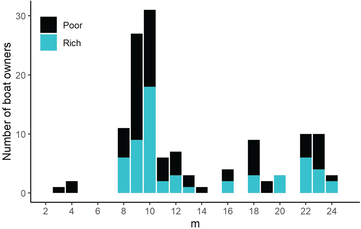
Fig. 3. Distribution of boat lengths, differentiated according to fishers’ wealth (rich vs poor).
2.3. Risk, uncertainty and coping strategies
As discussed above, income from fishing is volatile (see figure 2) and different income realizations are possible. If the distribution of these different states are known, we refer to ‘risk’; if this is not the case, we talk about ‘uncertainty’ (see, e.g., Knight, Reference Knight1921). Part of the volatility and the uncertainty stems from weather conditions. Weather varies daily and seasonally, but a certain regularity in average wind speeds over the course of the year (see figure 6 in section 2.5) prevails such that we assume that fishers have a fairly good idea about the distribution of the potential states.
In the detailed survey at the beginning of the study, all fishers state that variations in weather (wind, rain, temperature, waves, etc.) influence the availability of fish. In particular, 64 per cent of the respondents state that more wind entails less fish, while 22 per cent related more wind to more fish and the remaining either saw no change or changes in species.
To reduce uncertainty and volatility ex-ante, fishers can adapt their fishing strategies up to a certain extent by changing fishing effort and fishing gear.Footnote 9 Accordingly, while fishers cannot influence weather conditions, they can, to some extent, influence the risk they face from it. In the short run, fishers can adapt the amount of effort (number of fishing days) to adapt to this risk. In the longer run, they can choose the boat type, which is in our sample represented by the length of the boat. The boat length varies from 3 to 24 meters, with a median of 10 meters length with no significant differences between different locations. Longer boats imply more stability under rougher weather conditions, but also a higher economic risk as longer boats are more expensive. While fishers can vary the amount of effort (fishing days and length of fishing trips) from month to month, most fishers have only one boat and can hence only adapt their boat choice in the long-term.
In principle, fishers could also get an insurance contract against weather related risks; however, this is not very common among Senegalese fishers. Only two fishers have any insurance contract at all, but unrelated to weather. It is more common to save in order to have a buffer for hard times. Nearly 60 per cent of the fishers do this, while nearly all of those who do not save state that this is because they do not have enough money to save. Half of the ones that save, do so for a specific purpose like a wedding or major repairs or gear replacement, and the other half see saving as a general buffer for difficult times.
Taking out a loan is a typical way to react to shocks ex-post. In general, credit is available for Senegalese fishers. At the time of the initial survey (spring 2015), 39.5 per cent of the fishers were indebted, with 1.4 loans on average. Additional ways to deal with risks are interlinked loans (see, e.g., Riekhof, Reference Riekhof2019) or social sharing systems. Both also prevail in some locations on the Senegalese coast.
2.4. Data on risk-taking
The mean investment from the investment task per fisher is depicted in figure 4. Risk-neutral agents would maximize expected income and would invest the entire amount of 1200 FCFA. In our investment task, risk-loving behavior would look identical. Any investment below 1200 FCFA depicts risk-averse behavior. Figure 4 shows that participants generally behave in a risk-averse way. On average, fishers invested 60 per cent of the money they received each month. The observed risk-averse behavior is in line with the literature saying that particularly poor individuals will generally behave in a risk-averse manner (see, e.g., Kremer et al., Reference Kremer, Lee, Robinson and Rostapshova2013).

Fig. 4. Frequency of mean investment values per month.
We also briefly consider the stability of investments in the investment task over time. If all fishers are risk-averse and take the investment decision independent from the environment, each person will invest an identical amount that is lower than 1200 FCFA each month. We find that investments in the investment task vary considerably from month to month. This is true on average – aggregated (see figure 5) – as well as per fisher: the difference between the maximum invested and the minimum ever invested was at least 600 FCFA for 68 per cent of the participants. The mean of the coefficient of variation of the individual participants is 0.3, with a minimum of 0 (always the same investment) and a maximum of 0.8.

Fig. 5. Average investments in the investment task with error band (one standard deviation) over time.

Fig. 6. Comparison of monthly average wind speeds.
2.5. Background risk and data on wind conditions
To capture background risk, we construct a new measure based on wind speed. It builds on the following idea: fishers form expectations about the weather conditions and resulting income risks in a given month or over the course of the year based on their experience, which is based on past seasonal variations. Note that we cannot distinguish between health risk from higher wind speed and risk to fishing income from higher wind speed (lower fish availability and risk of damage to gear). However, since both risks go in the same direction, i.e., more wind, more risk, we can ignore this difference. Thus, to measure background risk, we take the average monthly wind speed in $m/s$ close to the coast of Senegal.Footnote 10 The data are taken from the U.S. Department of Commerce, National Oceanic and Atmospheric Administration Earth Systems Research Laboratory.Footnote 11 They indicate the monthly mean wind speed calculated from daily wind speed (from daily vector winds) from 1948/01 to the present. We take the longitude closest to the Senegalese coast and then differentiate between north and south of Dakar for the latitudes. We use the wind speed that prevailed at the surface of the sea (pressure ${>}925$
 ). Figure 6 depicts the monthly average wind speeds for the months of the study, as well as longer-run averages.
To capture expectations on wind speed in a given month, we think that considering the last 30 years (approximately one generation) is an appropriate period for expectation formation, because of the nature of learning that is happening in this sector. Most fishers learn fishing from their parents and continue to use the same rules of thumb as their parents. Advisory services are also slow in changing their recommendations. Evidence from the agricultural sector shows that changes in behaviors and methods are particularly slow, when the ideal particular behavior or method is not uniform across individuals (Foster and Rosenzweig, Reference Foster and Rosenzweig1995; Suri and Udry, Reference Suri and Udry2022).
As a measure of the certainty of the expected wind speed per month, we use the variability of wind speed in a given month over the years. For this, we calculate the standard deviation for each month, based on past yearly averages (see figure A1 in the online appendix that depicts average monthly wind speeds plus the standard deviations). A higher value indicates that there has been more variation, implying that a prediction for the month's wind speed based on past experiences is less accurate.
3. Empirical approach
We use fixed effects panel regression analysis to examine how background risk and disposable income impact risk-taking. Our empirical strategy depends on: (i) the panel structure of the data, (ii) the exogenous variation in background risk measured by wind conditions, and (iii) independence of the investment risk through a lab-in-the-field setting. We control for time-invariant differences between fishers and examine how the behavior of the individual fisher changes. Wind conditions are described by the average monthly wind speed based on time series data. The expected wind speed (based on the 30-year average) can be seen as a measure for background risk as higher wind speed makes fishing more risky.
Also, we have to take into account that the danger arising from higher wind speed is related to the size of boat. The wind speed is used as an instrument for the fishers’ perception of variability in income and probability of accidents. According to the knowledge and experience of our local partners, the relation between wind speed and vessel size is complex. Larger vessels are less susceptible to high wind speeds, but often fish further away from the coast and are thus less flexible in returning as a response to weather changes. Still, overall, it is likely that they face lower background risk as compared to smaller boats.
To examine the influence of background risk on the investment decision – potentially suggesting temperate or intemperate behavior – we estimate the following empirical model with subscripts $i$ and $t$
 relating to different fishers and months, respectively:

with household fixed effects – denoted by $\alpha _{i}$ – controlling for preferences and other unobservables at the household level that are constant over time; the term $X_{i,t}$
 collecting variables that control for external time varying factors; and the error term $\epsilon _{i,t}$
 .
.
In the following, we describe the variables in more detail. The dependent variable “Investment share$_{i,t}$ ” is the share of the total amount in FCFA received that fisher $i$
 invested in month $t$
 in the investment task. Our independent variable of interest is “Wind speed$_{t}$
 ” as a measure for background risk in month $t$
 . It is described in more detail in section 2.5. We interact wind speed with “Boat length$_{i}$
 ”, i.e., the length of fisher $i$
 's boat. “Log food exp per pP$_{i,t}$
 ’ is a measure for disposable income and indirectly for a realized shock. The interpretation is that when basic needs are covered, food expenditures go up due to spending on higher quality or more diverse food.Footnote 12 We divide the food expenditure by the household size to take into account that larger households require a higher income to have the same per-person expenditure as smaller households. We take logs, so that we can interpret results in terms of percentage change.
Controls, collected in $X_{i,t}$ in (1), include a dummy to control for date differences between when the interview took place and the month it relates to (the corresponding variable is called ‘Date difference’),Footnote 13 a dummy for the rainy season (June to October, called ‘Rainy season’) and a dummy for the tabaski ‘festival’, during which fishers usually do not go out for fishing (called ‘Tabaski’). Also, we include the average fishing income over all fishers in a month in logs (called ‘Mean fishing income (t)’) to control for level effects.Footnote 14 Except for ‘Date difference’, which depends on the individual and on time, the control variables only depend on time.
Descriptive statistics are in table A1 in the online appendix.
4. Results
Table 1 shows the main panel regression results for considering the impact of background risk measured by wind speed on investment. We use fixed effects with error terms clustered at the household level as preferred specification.Footnote 15
Table 1. Main panel regression results

Notes: p-values in parentheses. With fixed effects and error term clustered at the household level.
Column (1) shows a positive significant impact from the wind speed on investment, i.e., intemperate behaviour. Column (2) shows the importance of taking the impact of boat length into account: the impact becomes negative, but insignificant. The impact from wind speed interacted with boat length on investment, in turn, is significant and positive. Column (3) shows that the impact from wind speed on risk-taking is also negative, but insignificant, when exchanging the interaction terms for other appropriate controls. Column (4) is our main specification that includes relevant controls. It shows that a higher mean wind speed leads to lower investment, but that this effect is lower, and partly reversed, for fishers with longer boats. Reported boat lengths are between 3 and 24 meters, with two clusters around 8–10 meters as well as 22-23 meters. If the mean wind speed is increased by one standard deviation (1.9), investment is reduced by 2.4 percentage points for fishers with boats of 9 meter length, e.g., from 60 to 57.6 per cent. For fishers with a 23-meter boat, investment is increased by 0.85 percentage points. Figure 7 illustrates the marginal effects.

Fig. 7. Marginal effects of background risk and vessel size on risk-taking. Results are based on table 1, column (4), with an error band (one standard deviation).
Food expenditure per person is positively and significantly correlated with investment, suggesting that disposable income is relevant for short-term investment. As food covers a basic need, having more of this need covered increases additional risk-taking: A 1 per cent increase in the food expenditure per person increases the investment in the investment task by approximately 4.3 percentage points (see column (4) of table 1). Negative income shocks would also be reflected in this variable. These are often found to impact risk-taking (see, e.g., Chuang and Schechter, Reference Chuang and Schechter2015). In summary, at first sight, our findings suggest that fishers are on average intemperate. However, as soon as we add controls, results suggest temperate behavior for most fishers.
To better understand our results, we split our sample into the richer and the poorer half of the households in our sample. We denominate these two halves ‘rich (wealth)’ and ‘poor (wealth)’ in the following. It should be noted that these terms are only valid in the context of the dataset. Overall, all fishers in the sample belong to the poorer part of the Senegalese population. The idea is to test whether households that are strongly constrained financially, with basically no disposable income left after deducting the absolutely necessary, may behave differently from households that are less liquidity constrained, similarly to Guiso and Paiella (Reference Guiso and Paiella2008). To run the regressions for the rich and poor separately, we divide the sample according to the median of the wealth index that we described in section 2.2.
We find that higher wind speed per month as a measure for background risk has a negative effect on investment for both rich and poor (see columns (5) and (6) of table 1), but the effect is only significant for the poor. When interacted with boat length, the effect is positive, but only significant for the rich group. These results indicate temperate behavior for the poorer group and intemperate behavior for the richer group. In the latter case, the impact is increasing in boat length.
We also check whether richer fishers simply have larger boats. Figure 3 shows the number of observations by boat length for all respondents and for the wealthier half. While the very small boats are concentrated among the poorer part of the sample, there is no clear relationship between wealth and boat length for boats of eight meters and more.
Results indicate that fishers differ in their reaction to wind speed and that this is at least partly driven by their wealth level, but the results also point to another factor of relevance, that is the length of the boat. While longer boats are more stable in stronger winds, they also carry a larger crew and more fish, hence reducing the impact of wind, but increasing potential loss, although not necessarily per person. Figure A2 in the online appendix shows a negative relation between boat length and variability in fishing income (measured as Coefficient of Variation), which suggests that larger boats may indeed experience lower background risks at a given wind speed compared to smaller boats. Still, the graph is only based of few observations due to missing values.Footnote 16
Also, the impact from food expenditure per person becomes insignificant for the poorer group. The reason could be that for the poor, disposable income may be close to a lower minimum such that it is comparably stable and thus exhibits no influence on risk-taking over time. This is consistent with the result that for the rich, the coefficient of log food expenditure per person increases compared to the baseline, i.e., higher disposable income translates into even higher risk-taking in investment.
Our general summary and interpretation of our findings are as follows. For poorer fishers, higher background risk – measured as monthly expected wind speed, i.e., monthly wind speed – reduces independent risk-taking – measured by investment in the investment task. It seems that poorer fishers substitute different risks and are only willing to bear a certain level of risk. If background risk increases, they play safe(r) in independent risk-taking. For richer fishers, the results are the opposite. They react to a higher level of exogenous risk by also increasing independent risk-taking. It seems like they try to counteract potentially higher losses in one area by potentially higher gains in the other. Poorer fishers show temperate behavior, they substitute different risks, while richer fishers show intemperate behavior. We interpret our results as evidence that the direct economic situation is linked to temperance in behavior.
Before we discuss potential policy implications of our results, we present some robustness checks in the next section.
5. Robustness
The sensitivity of our results is tested in two ways. First, we check whether environmental conditions impact fishing days, i.e., the exposure to background risk. If fishers reduce the number of fishing days when wind speed is higher, they reduce their exposure to the calculated monthly background risk, i.e., they face a lower background risk. Second, we implement several robustness checks and additional regressions related to our baseline specification.
To see whether fishers react to higher expected monthly wind speed by reducing their fishing-days and thus their exposure to increased background risk, we take fishing days as dependent variable. Table A2 in the online appendix shows that fishing days are not impacted by mean wind speed (the coefficient is generally negative, but not significant). In addition to running the regression with the same explanatory variables as to explain investments before, we also run a regression in which we exclude ‘Log food exp per person’ (column (4)). The reason is potential reverse causality: fishing days influence fishing income, which influences food expenditure. The results are robust to the exclusion of the variable.Footnote 17 Results also show no difference between the poorer and the richer group of fishers (columns (5) and (6)).
We present the most interesting additional panel regression results in table 2. First, we add further controls (see column (1)): a time trend, a dummy whether the household has an additional income source, and the expected income next month. The time trend picks up potential underlying developments over time. The other variables relate to possible compensating mechanisms for income volatility, a kind of implicit ‘insurance’. Additional income sources may serve as a buffer for low fishing income and thus reduce the vulnerability to low realized fishing income. A high expected income for the ensuing month – measured as the mean fishing income, only for the ensuing month – may also lower the burden of a low current income and makes it easier to bear risks, compared to a situation with a low expected income. This, in turn, may then influence risk-taking. We also add the standard deviation around the long-run mean alone and interacted with boat length. The standard deviation around the long-run mean is a measure of certainty: how certain are the expectations on wind conditions in a month. This may influence risk-taking in the investment task.
Table 2. Further panel regression results as robustness check

Note: p-values in parentheses.
While our main results are robust to adding controls, results on the impact from the standard deviation around the long-run mean of wind speed and risk-taking on the investment task are noteworthy: the standard deviation has the opposite effect on risk-taking than the mean. The fishers increase risk-taking when the standard deviation of monthly wind speed increases, i.e., when there is a higher uncertainty surrounding the expected wind conditions.
We also examine whether the standard deviation of long-run wind conditions impact fishing days. Table A2 in the online appendix shows that the standard deviation has a negative effect on fishing days for all fishers, suggesting that fishers reduce their exposure when wind conditions are less certain, but the impact is not significant.
In addition, we check whether changing the reference period for wind speed changes the results. Tables A4 and A3 in the online appendix show the main results when using 67 years (the full available sample) and 10 years respectively as a reference period. There are no relevant changes with respect to our main variables of interest.
6. Discussion and conclusion
Fishers frequently have to take decisions involving risk, facing additional, independent risks, so-called background risks. Especially in low-income countries, many risks are often not insurable. We show that risk-taking of Senegalese fishers varies over time and is influenced by background risk as measured by wind conditions. Higher wind speeds usually imply more dangerous fishing conditions and less fish, and thus higher health and income risks. As the impact of wind speed on the fishers depends on their boat size, we take this into account and show that it has indeed an impact. Our results suggests that poorer fishers decrease risk-taking when background risk goes up, i.e., when wind speeds are higher, while richer fishers increase risk-taking. They do so even more when they have longer boats. One could say that poorer fishers substitute different risks and are only able to bear a certain amount of overall risks, while richer fishers try to compensate higher risk in one area by also taking more risk in another area. Overall, our results suggest that the impact of background risk on risk-taking depends on the socio-economic situation, as well as conditions relating to the activity itself which may impact the background risk experienced.
Our results complement the existing picture of risk behavior of households in developing countries in several ways, with implications for designing policies as well as investment and insurance products. First, we find that immediately available income and wealth are important determinants of risk-taking, confirming existing evidence (e.g., Guiso and Paiella, Reference Guiso and Paiella2008; Cardak and Wilkins, Reference Cardak and Wilkins2009). When available income and wealth are higher, fishers invest more easily. Second, we add to the growing evidence on the instability of risk-taking. Specifically, our analysis considers how variation in background risks and environmental conditions affects risky choices over time.
The fishers we studied currently experience increasing demand for fish, leading to rising fish prices. In addition, climate change and global warming often lead to higher wind speed, thus increasing background risk. If our results allow generalization, they show that there is a direct link between background risk as well as effort in current occupations (in our case fishing days) and diversification (in our case risk-taking). Both, exploiting market opportunities and responding to increasing climate risk, demand investments to adapt to these new circumstances. Investments could relate to short-run solutions, like changes in gear (e.g., fishing nets), motors, GPS devices or boats, or to longer-run investments that target income diversification (e.g., investments in agriculture or education). As in other countries, the traditional Senegalese fishery sector largely lacks these investments (Ba et al., Reference Ba, Schmidt, Déme, Lancker, Chaboud, Cury, Thiao, Diouf and Brehmer2017). We contribute to a better understanding of why unrealized investment opportunities prevail.
For investment promoting policy measures our results mean that higher disposable incomes increase risk-taking and hence investment in adaptation measures. Hence, raising incomes is an obvious strategy, but often not an easy one to implement. Our unique data also show that the poor seem to substitute different forms of risks. For policy makers, this implies that insurance mechanisms for the poor matter. Insurance mechanisms for investments in adaptation or innovations could solve this dilemma, provided that they are credible. In this line, Cole et al. (Reference Cole, Giné and Vickery2017) show that the provision of a rainfall insurance induces farmers to invest more in higher-return but climate-sensitive cash crops. However, the varied experience from weather index insurance (see, e.g., Giné and Yang, Reference Giné and Yang2009; Karlan et al., Reference Karlan, Osei, Osei-Akoto and Udry2014) shows that it is not easy to implement such insurances. Potentially more costly alternatives include cash transfers or a basic-needs social security system (Jensen et al., Reference Jensen, Barrett and Mude2017), which act as an insurance against very low income states.
Also, the timing of investment possibilities may be more relevant than previously supposed. For fishers, there are better and worse times for risk-taking, which are related to seasonality and weather patterns, translating into differences in disposable income and background risk. If new (fishing) methods are introduced, poorer fishers may find it easier to experiment with these when background risks are lower and when incomes are higher. As risk-taking is not stable over time, the right timing of a policy may increase its acceptance and its impact.
While our main finding relates to the impact of background risk on independent risk-taking in the Senegalese fishery, we also explore the role of background uncertainty on behavior as part of our sensitivity analysis. We explore background uncertainty in the sense that we include the variability of wind conditions in certain months over previous years. A higher past variability means that wind conditions are more difficult to predict, thus, one could say that uncertainty is higher. Our results suggest that one major reaction is to reduce exposure to these uncertain conditions. One could explore this effect and behavior under background uncertainty in general in more detail using, e.g., data related to the Covid pandemic.
Supplementary material
The supplementary material for this article can be found at https://doi.org/10.1017/S1355770X22000274
Acknowledgments
We would like to thank Aliou Ba, Lorena Fricke, Julia Hoffmann, Kira Lancker and Jörn Schmidt for support with the data. We also thank Stefan Baumg ärtner, Hans Gersbach, Christian Gollier, Michael Haliassos, Bentley MacLeod, Wanda Mimra, Martin Quaas, Uli Schmidt, Max Stoeven, Christian Waibel and participants at the PegNET conference 2017 as well as at seminars in Zurich and Kiel for helpful comments.
Conflict of interest
The authors declare none.


 Open access