


Impact Statement
A significant part of the U.K. rail and highway infrastructure is built on high-plasticity clay soils which have an increased risk of failure. We have performed computer simulations of slope deterioration to determine the relationship between their time to failure and slope geometry, soil strength, and permeability. However, the simulations are very time-consuming. This can be addressed by using statistical surrogate models which are trained to be similar to computer simulator output. The surrogate can perform time to failure predictions for hundreds of slope geometry and strength combinations within hours, compared with years of computational time using the original simulator. The trained surrogate could be used to inform slope design, management, and maintenance on different spatio-temporal scales of transport networks.
1. Introduction
The U.K. transport infrastructure is crucial to the efficient functioning of the economy and society. In particular, rail transportation is crucial to securing efficient and low-carbon logistical services to individuals and businesses; road transport will also continue to play a significant role in the future. A significant part of the U.K. rail infrastructure is nearing 200 years in age while being built on/within high-plasticity soils that are prone to weathering and deterioration. A section of the U.K. Great Western Main Line route connecting London to Bristol is one of the busiest and oldest (ca. 170 years post-construction) rail corridors in the United Kingdom (Skempton, Reference Skempton1996) that has undergone significant deterioration over its life cycle. Earthworks on the highways suffer from similar problems but to a lesser extent because of their relatively recent construction dates (1950s onwards) and shallower slope angles and heights. A lack of understanding of the long-term behavior, performance, and deterioration of infrastructure slopes can lead to uncontrolled deformations and thus reduced service performance (Briggs et al., Reference Briggs, Dijkstra and Glendinning2019), negative impact on the economy (Power and Abbott, Reference Power and Abbott2019), and, in the worst case, fatalities (Smith, Reference Smith2020). Here, we aim to reduce the risks posed to infrastructure systems by better understanding the deterioration of geological assets.
Deterioration processes have been studied through computer experiments (Stirling et al., Reference Stirling, Glendinning and Davie2017; Wang et al., Reference Wang, Chong, Xu and Pan2018) but these are computationally expensive and time-consuming (Maatouk and Bay, Reference Maatouk and Bay2017). Instead, we use surrogate statistical models, which can be used to approximate computationally burdensome computer code/simulators, based on a small number of simulator runs at well-selected input locations (O’Hagan, Reference O’Hagan2006).
A simulator can be represented by a function $ f $
evaluated at input variables
$ f $
evaluated at input variables $ \boldsymbol{x} $
to produce outputs
$ \boldsymbol{x} $
to produce outputs $ \boldsymbol{y} $
,
$ \boldsymbol{y} $
, $ f\left(\boldsymbol{x}\right)=\boldsymbol{y} $
. The term “emulator” (O’Hagan, Reference O’Hagan2006) was originally coined to refer to statistical approximations of a simulator which provide a probability distribution of its output. Gaussian processes (GPs) are one of the most frequently used machine learning (e.g., Seeger, Reference Seeger2004; Rasmussen and Nickisch, Reference Rasmussen and Nickisch2010; Su et al., Reference Su, Yu, Xiao and Yan2016) and emulation techniques because of convenient properties such as uncertainty quantification (Maatouk and Bay, Reference Maatouk and Bay2017), conditional normality, and a flexibility in defining the mean and variance structure of the process. GPs are amenable to statistical inference using Bayesian methods (O’Hagan, Reference O’Hagan2006). This allows expert opinion to be easily incorporated, which is especially useful when modeling sparse data or computer simulators with high computational cost. Gaussian process emulators (GPEs) have been applied to a variety of problems, including models of microbial communities (Oyebamiji et al., Reference Oyebamiji, Wilkinson, Jayathilake, Curtis, Rushton, Li and Gupta2017), generic plant functional types (Kennedy et al., Reference Kennedy, Anderson, Conti and O’Hagan2006), cardiac cells (Chang et al., Reference Chang, Strong and Clayton2015), and stochastic economic dispatch (Hu et al., Reference Hu, Xu, Korkali, Chen, Mili and Tong2020). Gaussian process emulation was also used to estimate the probability of soil slope failure in a non-Bayesian setting (Kang et al., Reference Kang, Han, Salgado and Li2015).
$ f\left(\boldsymbol{x}\right)=\boldsymbol{y} $
. The term “emulator” (O’Hagan, Reference O’Hagan2006) was originally coined to refer to statistical approximations of a simulator which provide a probability distribution of its output. Gaussian processes (GPs) are one of the most frequently used machine learning (e.g., Seeger, Reference Seeger2004; Rasmussen and Nickisch, Reference Rasmussen and Nickisch2010; Su et al., Reference Su, Yu, Xiao and Yan2016) and emulation techniques because of convenient properties such as uncertainty quantification (Maatouk and Bay, Reference Maatouk and Bay2017), conditional normality, and a flexibility in defining the mean and variance structure of the process. GPs are amenable to statistical inference using Bayesian methods (O’Hagan, Reference O’Hagan2006). This allows expert opinion to be easily incorporated, which is especially useful when modeling sparse data or computer simulators with high computational cost. Gaussian process emulators (GPEs) have been applied to a variety of problems, including models of microbial communities (Oyebamiji et al., Reference Oyebamiji, Wilkinson, Jayathilake, Curtis, Rushton, Li and Gupta2017), generic plant functional types (Kennedy et al., Reference Kennedy, Anderson, Conti and O’Hagan2006), cardiac cells (Chang et al., Reference Chang, Strong and Clayton2015), and stochastic economic dispatch (Hu et al., Reference Hu, Xu, Korkali, Chen, Mili and Tong2020). Gaussian process emulation was also used to estimate the probability of soil slope failure in a non-Bayesian setting (Kang et al., Reference Kang, Han, Salgado and Li2015).
The following assumptions are made in order for $ f\left(\boldsymbol{x}\right) $
to be represented by a GPE. It is assumed that
$ f\left(\boldsymbol{x}\right) $
to be represented by a GPE. It is assumed that $ f\left(\boldsymbol{x}\right) $
is a smooth, continuous function of its input variables (O’Hagan, Reference O’Hagan2006) and that outputs of
$ f\left(\boldsymbol{x}\right) $
is a smooth, continuous function of its input variables (O’Hagan, Reference O’Hagan2006) and that outputs of $ f\left(\boldsymbol{x}\right) $
for any sequence of inputs can be modeled as a multivariate normal distribution with mean and covariance functions depending on the inputs. Although assuming normality is restrictive to some extent, this is offset by the great flexibility in the choice of mean and covariance functions (Gramacy, Reference Gramacy2020).
$ f\left(\boldsymbol{x}\right) $
for any sequence of inputs can be modeled as a multivariate normal distribution with mean and covariance functions depending on the inputs. Although assuming normality is restrictive to some extent, this is offset by the great flexibility in the choice of mean and covariance functions (Gramacy, Reference Gramacy2020).
According to O’Hagan (Reference O’Hagan2006), an emulator should satisfy two criteria. First, the emulator has no uncertainty in the output $ {\boldsymbol{y}}_i=f\left({\boldsymbol{x}}_i\right),i=1,2,\dots, n $
evaluated at a simulator input
$ {\boldsymbol{y}}_i=f\left({\boldsymbol{x}}_i\right),i=1,2,\dots, n $
evaluated at a simulator input $ {\boldsymbol{x}}_i $
. Second, elsewhere the emulator gives a distribution of plausible interpolated values. The first condition is often relaxed in practice (Gramacy, Reference Gramacy2020) by adding
$ {\boldsymbol{x}}_i $
. Second, elsewhere the emulator gives a distribution of plausible interpolated values. The first condition is often relaxed in practice (Gramacy, Reference Gramacy2020) by adding $ \tau $
to the diagonal of the covariance matrix, where
$ \tau $
to the diagonal of the covariance matrix, where $ \tau $
is a small number known as the nugget. The latter can account for an uncertainty/error in the simulator output (Cressie, Reference Cressie1993) or improve numerical stability when inverting the covariance matrix of the GPE (Neal, Reference Neal1997) which may appear numerically ill-conditioned (Gramacy, Reference Gramacy2020). Further discussion on the use of the nugget term and its effect can be seen in, for example, Andrianakis and Challenor (Reference Andrianakis and Challenor2012).
$ \tau $
is a small number known as the nugget. The latter can account for an uncertainty/error in the simulator output (Cressie, Reference Cressie1993) or improve numerical stability when inverting the covariance matrix of the GPE (Neal, Reference Neal1997) which may appear numerically ill-conditioned (Gramacy, Reference Gramacy2020). Further discussion on the use of the nugget term and its effect can be seen in, for example, Andrianakis and Challenor (Reference Andrianakis and Challenor2012).
In this paper, we use a GPE to approximate computer experiments with 76 geotechnical simulator runs of infrastructure slope deterioration that would otherwise be infeasibly time-consuming to evaluate. The experimental results presented here are focused on the slopes in high to very high-plasticity soils, such as slopes in the London Clay (Hight et al., Reference Hight, McMillan, Powell, Jardine and Allenou2003). While over 40 model inputs can be varied (FLAC, 2016; Rouainia et al., Reference Rouainia, Helm, Davies and Glendinning2020; Postill et al., Reference Postill, Helm, Dixon, Glendinning, Smethurst, Rouainia, Briggs, El-Hamalawi and Blake2021), here we only vary slope geometry (angle and height), soil shear strength (cohesion and friction angle), and permeability. These variables were selected over the remaining ones as previous work has demonstrated their importance in assessing the stability of geotechnical infrastructure (Potts et al., Reference Potts, Kovacevic and Vaughan1997; Ellis and O’Brien, Reference Ellis and O’Brien2007; Rouainia et al., Reference Rouainia, Helm, Davies and Glendinning2020). This allows us to limit the experimental time to weeks while obtaining an informative training data set. To ensure an optimal coverage of the parameter space, a Latin hypercube experimental design is used. The simulator runs were stopped after 184 years of model time, corresponding to the average rail cutting slope age in the London–Bristol corridor (Skempton, Reference Skempton1996). Slopes that have not failed within this time have their time to failure (TTF) censored. In such cases, our GPE imputes the uncensored TTF.
The structure of this article is as follows. Section 2 describes the computer experiments and geotechnical model (GM) that simulate deterioration processes in cut slopes. Section 3 outlines the background related to the emulator, Bayesian inference, and emulating the censored computer output. Section 4 presents the results of Markov chain Monte Carlo (MCMC) inference of the GPE posterior distribution and related sensitivity analysis. Section 5 discusses the TTF predictions for a range of cutting slope geometry and soil strength scenarios as well as for London–Bristol corridor railway and M4 motorway cuttings. Finally, Section 6 concludes the study and outlines future directions for research.
2. Application: Computer Experiments of Cut Slope Deterioration
2.1. Introduction
The Great Western Main Line (GWML) and the M4 motorway corridors are constructed through a number of geological formations, a significant proportion of which are comprised of over-consolidated and high-plasticity clays (Charlesworth, Reference Charlesworth1984; Skempton, Reference Skempton1996). These materials are prone to seasonal shrink–swell movements as they wet and dry, along with downslope ratcheting (Take and Bolton, Reference Take and Bolton2011), both of which contribute to strain softening (Rouainia et al., Reference Rouainia, Helm, Davies and Glendinning2020; Postill et al., Reference Postill, Helm, Dixon, Glendinning, Smethurst, Rouainia, Briggs, El-Hamalawi and Blake2021) reducing their strength over time. With the GWML and M4 earthworks that are of ca. 175 and 65 years of age, respectively, the soils from which they are formed will have been subject to a varying number of these seasonal cycles and undergone an indeterminate magnitude of deterioration from their initial state. Here, we focus on replicating these deterioration processes in high-plasticity, over-consolidated clays, particularly London Clay (Hight et al., Reference Hight, McMillan, Powell, Jardine and Allenou2003; Dixon et al., Reference Dixon, Crosby, Stirling, Hughes, Smethurst, Briggs, Hughes, Gunn, Hobbs, Loveridge, Glendinning, Dijkstra and Hudson2019; Rouainia et al., Reference Rouainia, Helm, Davies and Glendinning2020).
The time-dependent stability of cut slopes has been the subject of previous numerical modeling work (Potts et al., Reference Potts, Kovacevic and Vaughan1997; Tsiampousi et al., Reference Tsiampousi, Zdravkovic and Potts2017; Summersgill et al., Reference Summersgill, Kontoe and Potts2018). Capturing the influence of weather and seasonal cycles, as well as the strain-softening behavior is crucial to the accurate modeling of over-consolidated high-plasticity clays.
2.2. The GM
This subsection is a summary of the key mechanisms and properties that influence the slope deterioration behavior in the GM used in our simulator. For more detail, see Rouainia et al. (Reference Rouainia, Helm, Davies and Glendinning2020) and Postill et al. (Reference Postill, Helm, Dixon, Glendinning, Smethurst, Rouainia, Briggs, El-Hamalawi and Blake2021).
The GM is implemented using the Fast Lagrangian Analysis of Continua with Two-Phase Flow software (FLAC-TP; FLAC, 2016), making use of a strain-softening Mohr–Coulomb constitutive model (FLAC, 2016). The parameters adopted in the modeling have been informed by the strain-softening behavior from previous modeling studies in over-consolidated clays (Potts et al., Reference Potts, Kovacevic and Vaughan1997; Ellis and O’Brien, Reference Ellis and O’Brien2007; Summersgill et al., Reference Summersgill, Kontoe and Potts2018) as well as laboratory and field data (Bromhead and Dixon, Reference Bromhead and Dixon1986). The impact of weather and climate on cut slopes is modeled through a coupled fluid-mechanical approach (Rouainia et al., Reference Rouainia, Helm, Davies and Glendinning2020) utilizing a nonlocal strain-softening model (Summersgill et al., Reference Summersgill, Kontoe and Potts2018; Postill et al., Reference Postill, Helm, Dixon, Glendinning, Smethurst, Rouainia, Briggs, El-Hamalawi and Blake2021). This allows a detailed assessment of weather-driven deterioration.
The soil is modeled as a porous medium with variable saturation and depth-dependent saturated permeability (Postill et al., Reference Postill, Helm, Dixon, Glendinning, Smethurst, Rouainia, Briggs, El-Hamalawi and Blake2021). A two-phase flow approach is adopted where the pore phases are assumed to be air and water and are treated as immiscible fluids with differing density and viscosity. Fluid flow is Darcian, whereby water and air flow velocity is a function of the respective pore fluid pressures and the relative permeability of the soil. The latter, in turn, is a function of the degree of water and air saturation, derived using the van Genuchten–Maulem relation (van Genuchten, Reference van Genuchten1980).
The constitutive model is nonlinear elastic where the bulk and shear moduli behave as a function of the mean effective stress. These parameters were adopted from prior modeling studies (Potts et al., Reference Potts, Kovacevic and Vaughan1997; Jurečič et al., Reference Jurečič, Zdravković and Jovičić2013) and the stiffness behavior is validated in Postill et al. (Reference Postill, Helm, Dixon, Glendinning, Smethurst, Rouainia, Briggs, El-Hamalawi and Blake2021). The shear strength of high-plasticity clays undergoes a reduction as shear strain increases during yielding. This post-failure strength decrease is replicated in the model based on a reduction in the Mohr–Coulomb shear strength parameters (effective peak cohesion $ {c}^{\prime } $
and friction angle
$ {c}^{\prime } $
and friction angle $ {\phi}^{\prime } $
) as a function of increasing plastic shear strains. More details about the GM can be found in Rouainia et al. (Reference Rouainia, Helm, Davies and Glendinning2020) and Postill et al. (Reference Postill, Helm, Dixon, Glendinning, Smethurst, Rouainia, Briggs, El-Hamalawi and Blake2021).
$ {\phi}^{\prime } $
) as a function of increasing plastic shear strains. More details about the GM can be found in Rouainia et al. (Reference Rouainia, Helm, Davies and Glendinning2020) and Postill et al. (Reference Postill, Helm, Dixon, Glendinning, Smethurst, Rouainia, Briggs, El-Hamalawi and Blake2021).
2.2.1. Input variables
The five input variables in this study are the slope angle cotangent $ \cot {\theta}_s $
and height
$ \cot {\theta}_s $
and height $ {h}_s $
(converted to a single geometry variable—see Supplementary Figure S1) derived from light detection and ranging (LiDAR) survey data provided by project stakeholders (Mott MacDonald and Network Rail), the peak shear strength parameters (
$ {h}_s $
(converted to a single geometry variable—see Supplementary Figure S1) derived from light detection and ranging (LiDAR) survey data provided by project stakeholders (Mott MacDonald and Network Rail), the peak shear strength parameters ( $ {c}_p^{\prime } $
and
$ {c}_p^{\prime } $
and $ {\phi}_p^{\prime } $
) before the material has undergone any strength reduction derived from previous laboratory data and modeling studies (Apted, Reference Apted1977; Ellis and O’Brien, Reference Ellis and O’Brien2007), and the reference coefficient of permeability of the soil at 1 m depth with respect to water (
$ {\phi}_p^{\prime } $
) before the material has undergone any strength reduction derived from previous laboratory data and modeling studies (Apted, Reference Apted1977; Ellis and O’Brien, Reference Ellis and O’Brien2007), and the reference coefficient of permeability of the soil at 1 m depth with respect to water ( $ {k}_1^w $
) derived from field measurements (Dixon et al., Reference Dixon, Crosby, Stirling, Hughes, Smethurst, Briggs, Hughes, Gunn, Hobbs, Loveridge, Glendinning, Dijkstra and Hudson2019). For more information on the adopted GM and the values adopted for the remaining input parameters, see FLAC (2016), Rouainia et al. (Reference Rouainia, Helm, Davies and Glendinning2020), and Postill et al. (Reference Postill, Helm, Dixon, Glendinning, Smethurst, Rouainia, Briggs, El-Hamalawi and Blake2021).
$ {k}_1^w $
) derived from field measurements (Dixon et al., Reference Dixon, Crosby, Stirling, Hughes, Smethurst, Briggs, Hughes, Gunn, Hobbs, Loveridge, Glendinning, Dijkstra and Hudson2019). For more information on the adopted GM and the values adopted for the remaining input parameters, see FLAC (2016), Rouainia et al. (Reference Rouainia, Helm, Davies and Glendinning2020), and Postill et al. (Reference Postill, Helm, Dixon, Glendinning, Smethurst, Rouainia, Briggs, El-Hamalawi and Blake2021).
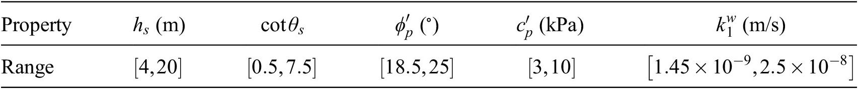
Table 1 summarizes ranges of the parameters used in computer simulations which were selected based on previous studies (Rouainia et al., Reference Rouainia, Helm, Davies and Glendinning2020; Postill et al., Reference Postill, Helm, Dixon, Glendinning, Smethurst, Rouainia, Briggs, El-Hamalawi and Blake2021) and expert opinion from partners in the ACHILLES project. During emulation, permeability was scaled by $ {10}^8 $
to bring the explanatory variables to a common scale. Supplementary Figure S1 illustrates that we have chosen geometries that are concentrated within the 4–12 m height and 1–4 angle cotangent ranges. This corresponds to the most common geometries in the London–Bristol corridor (Network Rail, 2017).
$ {10}^8 $
to bring the explanatory variables to a common scale. Supplementary Figure S1 illustrates that we have chosen geometries that are concentrated within the 4–12 m height and 1–4 angle cotangent ranges. This corresponds to the most common geometries in the London–Bristol corridor (Network Rail, 2017).
Table 1. Material and geometry input variables used in the computer experiments.
2.2.2. Model run time
The duration of the geotechnical modeling runs varied from approximately 75 min to 10 days. The latter depends on a number of factors, including the total number of elements in the model, model geometry, permeability, and the adopted strength parameters. For example, a model with the longest run time would correspond to a slope that is shallow enough to be stable for the full potential duration of the boundary time series and which includes a high near surface permeability yielding small flow time step. Conversely, the highest/steepest slope models tended to fail very quickly after modeled excavation.
3. Background
Here we review the methods which will be used for our GPE. Section 3.1 reviews GPEs, based on Bastos and O’Hagan (Reference Bastos and O’Hagan2009), Section 3.2 introduces the censored emulator model, Section 3.3 describes Bayesian inference and prediction for GPEs, Section 3.4 outlines our sensitivity analysis methods and Section 3.5 reviews Latin hypercube experimental design that we adopted for this study.
3.1. Gaussian process emulator
A GP can be understood as an infinite-dimensional multivariate normal distribution for functions (Bastos and O’Hagan, Reference Bastos and O’Hagan2009). A GPE $ \eta \left(\cdot \right) $
is a GP conditioned on experimental simulations that can be used to predict simulator output under other conditions, and quantify its uncertainty. Assume
$ \eta \left(\cdot \right) $
is a GP conditioned on experimental simulations that can be used to predict simulator output under other conditions, and quantify its uncertainty. Assume $ \eta \left(\cdot \right) $
takes a generic input
$ \eta \left(\cdot \right) $
takes a generic input $ \boldsymbol{x}=\left({x}_1,{x}_2,\dots, {x}_p\right) $
where
$ \boldsymbol{x}=\left({x}_1,{x}_2,\dots, {x}_p\right) $
where $ {x}_i\,\in\,{\chi}_i\,\subset\,\mathrm{\mathbb{R}} $
. A scalar-valued GP is fully defined by its mean and covariance functions
$ {x}_i\,\in\,{\chi}_i\,\subset\,\mathrm{\mathbb{R}} $
. A scalar-valued GP is fully defined by its mean and covariance functions $ m $
and
$ m $
and $ V $
,
$ V $
, $ \eta \left(\cdot \right)\mid \boldsymbol{\beta}, {\sigma}^2,\boldsymbol{\theta}, \tau \sim \mathrm{GP}\left(m\left(\cdot \right),V\left(\cdot, \cdot \right)\right) $
(Bastos and O’Hagan, Reference Bastos and O’Hagan2009).
$ \eta \left(\cdot \right)\mid \boldsymbol{\beta}, {\sigma}^2,\boldsymbol{\theta}, \tau \sim \mathrm{GP}\left(m\left(\cdot \right),V\left(\cdot, \cdot \right)\right) $
(Bastos and O’Hagan, Reference Bastos and O’Hagan2009).
Given no prior knowledge about the structure of $ m:{\mathrm{\mathbb{R}}}^p\to \mathrm{\mathbb{R}} $
, it is often assumed to be a linear transformation of the input variables, that is,
$ m:{\mathrm{\mathbb{R}}}^p\to \mathrm{\mathbb{R}} $
, it is often assumed to be a linear transformation of the input variables, that is, $ m\left(\boldsymbol{x}\right)=h{\left(\boldsymbol{x}\right)}^T\boldsymbol{\beta} $
, where
$ m\left(\boldsymbol{x}\right)=h{\left(\boldsymbol{x}\right)}^T\boldsymbol{\beta} $
, where $ h\left(\cdot \right):{\mathrm{\mathbb{R}}}^p\to {\mathrm{\mathbb{R}}}^q $
is a function mapping
$ h\left(\cdot \right):{\mathrm{\mathbb{R}}}^p\to {\mathrm{\mathbb{R}}}^q $
is a function mapping $ x $
to a vector of linear regressors and
$ x $
to a vector of linear regressors and $ \boldsymbol{\beta} =\left({\beta}_1,{\beta}_2,\dots, {\beta}_q\right) $
. To include a constant term in
$ \boldsymbol{\beta} =\left({\beta}_1,{\beta}_2,\dots, {\beta}_q\right) $
. To include a constant term in $ m\left(\boldsymbol{x}\right) $
, the first element of
$ m\left(\boldsymbol{x}\right) $
, the first element of $ h\left(\boldsymbol{x}\right) $
can be set to 1. We assume the covariance function
$ h\left(\boldsymbol{x}\right) $
can be set to 1. We assume the covariance function $ V:{\mathrm{\mathbb{R}}}^p\times {\mathrm{\mathbb{R}}}^p\to \mathrm{\mathbb{R}} $
has the form
$ V:{\mathrm{\mathbb{R}}}^p\times {\mathrm{\mathbb{R}}}^p\to \mathrm{\mathbb{R}} $
has the form $ V\left(\boldsymbol{x},{\boldsymbol{x}}^{\prime}\right)={\sigma}^2\left[C\left(\boldsymbol{x},{\boldsymbol{x}}^{\prime },\theta \right)+\tau \unicode{x1D540}\left(\boldsymbol{x},{\boldsymbol{x}}^{\prime}\right)\right] $
, where
$ V\left(\boldsymbol{x},{\boldsymbol{x}}^{\prime}\right)={\sigma}^2\left[C\left(\boldsymbol{x},{\boldsymbol{x}}^{\prime },\theta \right)+\tau \unicode{x1D540}\left(\boldsymbol{x},{\boldsymbol{x}}^{\prime}\right)\right] $
, where $ \sigma $
is a scale parameter,
$ \sigma $
is a scale parameter, $ C\left(\boldsymbol{x},{\boldsymbol{x}}^{\prime },\theta \right) $
is a correlation function,
$ C\left(\boldsymbol{x},{\boldsymbol{x}}^{\prime },\theta \right) $
is a correlation function, $ \tau $
is the nugget (Andrianakis and Challenor, Reference Andrianakis and Challenor2012), and
$ \tau $
is the nugget (Andrianakis and Challenor, Reference Andrianakis and Challenor2012), and $ \unicode{x1D540}\left(\boldsymbol{x},{\boldsymbol{x}}^{\prime}\right) $
is an indicator function for the event
$ \unicode{x1D540}\left(\boldsymbol{x},{\boldsymbol{x}}^{\prime}\right) $
is an indicator function for the event $ \boldsymbol{x}={\boldsymbol{x}}^{\prime } $
.
$ \boldsymbol{x}={\boldsymbol{x}}^{\prime } $
.
In principle, $ C $
can be any function that is smooth, continuous, and positive semidefinite. We consider two popular correlation functions. The first is the Gaussian function
$ C $
can be any function that is smooth, continuous, and positive semidefinite. We consider two popular correlation functions. The first is the Gaussian function $ {C}_G\left(\boldsymbol{x},{\boldsymbol{x}}^{\prime },\boldsymbol{\theta} \right)=\exp \left\{-{\sum}_{i=1}^p\frac{{\left({x}_i-{x}_i^{\prime}\right)}^2}{\theta_i^2}\right\} $
, where
$ {C}_G\left(\boldsymbol{x},{\boldsymbol{x}}^{\prime },\boldsymbol{\theta} \right)=\exp \left\{-{\sum}_{i=1}^p\frac{{\left({x}_i-{x}_i^{\prime}\right)}^2}{\theta_i^2}\right\} $
, where $ \boldsymbol{\theta} =\left({\theta}_1,{\theta}_2,\dots, {\theta}_p\right) $
is a vector of correlation lengths. The correlation lengths represent the “radius of association” and larger
$ \boldsymbol{\theta} =\left({\theta}_1,{\theta}_2,\dots, {\theta}_p\right) $
is a vector of correlation lengths. The correlation lengths represent the “radius of association” and larger $ \boldsymbol{\theta} $
values typically lead to smoother/flatter GPs. Second, we consider the Matérn correlation family (Rasmussen and Williams, Reference Rasmussen and Williams2006):
$ \boldsymbol{\theta} $
values typically lead to smoother/flatter GPs. Second, we consider the Matérn correlation family (Rasmussen and Williams, Reference Rasmussen and Williams2006):
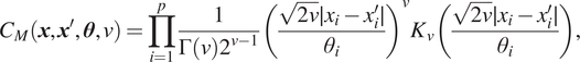 $$ {C}_M\left(\boldsymbol{x},{\boldsymbol{x}}^{\prime },\boldsymbol{\theta}, \nu \right)=\prod \limits_{i=1}^p\frac{1}{\Gamma \left(\nu \right){2}^{\nu -1}}{\left(\frac{\sqrt{2\nu}\mid {x}_i-{x}_i^{\prime}\mid }{\theta_i}\right)}^{\nu }{K}_{\nu}\left(\frac{\sqrt{2\nu}\mid {x}_i-{x}_i^{\prime}\mid }{\theta_i}\right), $$
where $ {K}_{\nu } $
is the modified Bessel function of second kind of order
$ {K}_{\nu } $
is the modified Bessel function of second kind of order $ \nu $
.
$ \nu $
.
As GPs are closed under conditioning, it is possible to derive an analytical expression for the GPE conditioned on a set of simulator runs. Assume a (finite) collection of $ n $
observed experimental outputs
$ n $
observed experimental outputs $ \boldsymbol{y}=\left(\eta \left({\boldsymbol{x}}_1\right),\eta \left({\boldsymbol{x}}_2\right),\dots, \eta \left({\boldsymbol{x}}_n\right)\right) $
performed on the inputs
$ \boldsymbol{y}=\left(\eta \left({\boldsymbol{x}}_1\right),\eta \left({\boldsymbol{x}}_2\right),\dots, \eta \left({\boldsymbol{x}}_n\right)\right) $
performed on the inputs $ {\boldsymbol{x}}_1,{\boldsymbol{x}}_2,\dots, {\boldsymbol{x}}_n $
, which comprise the training data. We assume no repeated inputs, so
$ {\boldsymbol{x}}_1,{\boldsymbol{x}}_2,\dots, {\boldsymbol{x}}_n $
, which comprise the training data. We assume no repeated inputs, so $ {\boldsymbol{x}}_i={\boldsymbol{x}}_j $
if and only if
$ {\boldsymbol{x}}_i={\boldsymbol{x}}_j $
if and only if $ i=j $
. The
$ i=j $
. The $ n $
-vector
$ n $
-vector $ \boldsymbol{y} $
follows a multivariate normal distribution,
$ \boldsymbol{y} $
follows a multivariate normal distribution, $ \boldsymbol{y}\mid \boldsymbol{\beta}, {\sigma}^2,\boldsymbol{\theta}, \tau \sim \mathrm{N}\left({H}_x\boldsymbol{\beta}, {\sigma}^2{\Sigma}_x\right) $
, where
$ \boldsymbol{y}\mid \boldsymbol{\beta}, {\sigma}^2,\boldsymbol{\theta}, \tau \sim \mathrm{N}\left({H}_x\boldsymbol{\beta}, {\sigma}^2{\Sigma}_x\right) $
, where $ {H}_x $
is a matrix of regressors whose
$ {H}_x $
is a matrix of regressors whose $ i $
th row is
$ i $
th row is $ h\left({\boldsymbol{x}}_i\right) $
and
$ h\left({\boldsymbol{x}}_i\right) $
and $ {\Sigma}_{x\left(i,j\right)}=C\left({\boldsymbol{x}}_i,{\boldsymbol{x}}_j,\boldsymbol{\theta} \right)+\tau \unicode{x1D540}\left(i,j\right) $
. Using standard rules for conditioning on a subset of observations (Gramacy, Reference Gramacy2020),
$ {\Sigma}_{x\left(i,j\right)}=C\left({\boldsymbol{x}}_i,{\boldsymbol{x}}_j,\boldsymbol{\theta} \right)+\tau \unicode{x1D540}\left(i,j\right) $
. Using standard rules for conditioning on a subset of observations (Gramacy, Reference Gramacy2020),
 $$ {\displaystyle \begin{array}{c}\eta \left(\cdot \right)\mid \boldsymbol{y},\boldsymbol{\beta}, {\sigma}^2,\boldsymbol{\theta}, \tau \sim \mathrm{GP}\left({m}^{\ast}\left(\cdot \right),{V}^{\ast}\left(\cdot, \cdot \right)\right),\mathrm{where}\\ {}{m}^{\ast}\left(\boldsymbol{x}\right)=h{\left(\boldsymbol{x}\right)}^T\boldsymbol{\beta} +t{\left(\boldsymbol{x}\right)}^T{\Sigma}_x^{-1}\left(\boldsymbol{y}-{H}_x\boldsymbol{\beta} \right),\hskip1.5pt {V}^{\ast}\left(\boldsymbol{x},{\boldsymbol{x}}^{\prime}\right)={\sigma}^2\left(C\left(\boldsymbol{x},{\boldsymbol{x}}^{\prime },\boldsymbol{\theta} \right)-t{\left(\boldsymbol{x}\right)}^T{\Sigma}_x^{-1}t\left({\boldsymbol{x}}^{\prime}\right)\right),\end{array}} $$
where $ t\left(\boldsymbol{x}\right)={\left(C\left(\boldsymbol{x},{\boldsymbol{x}}_1,\boldsymbol{\theta} \right),C\left(\boldsymbol{x},{\boldsymbol{x}}_2,\boldsymbol{\theta} \right),\dots, C\left(\boldsymbol{x},{\boldsymbol{x}}_n,\boldsymbol{\theta} \right)\right)}^T $
is a column vector of correlations between the (generic) emulator input
$ t\left(\boldsymbol{x}\right)={\left(C\left(\boldsymbol{x},{\boldsymbol{x}}_1,\boldsymbol{\theta} \right),C\left(\boldsymbol{x},{\boldsymbol{x}}_2,\boldsymbol{\theta} \right),\dots, C\left(\boldsymbol{x},{\boldsymbol{x}}_n,\boldsymbol{\theta} \right)\right)}^T $
is a column vector of correlations between the (generic) emulator input $ \boldsymbol{x} $
and training inputs
$ \boldsymbol{x} $
and training inputs $ {\boldsymbol{x}}_1,{\boldsymbol{x}}_2,\dots, {\boldsymbol{x}}_n $
.
$ {\boldsymbol{x}}_1,{\boldsymbol{x}}_2,\dots, {\boldsymbol{x}}_n $
.
3.2. Censored computer output
Censoring is a common phenomenon where only partial information is available on some observations, that is, it is only known that they are outside a specified range. A GPE can be conditioned on both censored and uncensored observations. Previous applications of censored GPs include hydrologic system response (Wani et al., Reference Wani, Scheidegger, Carbajal, Rieckermann and Blumensaat2017) and pyroclastic volcano flow (Kyzyurova, Reference Kyzyurova2017).
Censored values can be estimated together with $ \boldsymbol{\beta}, {\sigma}^2,\boldsymbol{\theta} $
and
$ \boldsymbol{\beta}, {\sigma}^2,\boldsymbol{\theta} $
and $ \tau $
using data augmentation during MCMC sampling. For our application, suppose
$ \tau $
using data augmentation during MCMC sampling. For our application, suppose $ n $
experiments at the set of inputs
$ n $
experiments at the set of inputs $ {\boldsymbol{x}}_o=\left({\boldsymbol{x}}_{o,1},{\boldsymbol{x}}_{o,2},\dots, {\boldsymbol{x}}_{o,n}\right) $
produced uncensored observations
$ {\boldsymbol{x}}_o=\left({\boldsymbol{x}}_{o,1},{\boldsymbol{x}}_{o,2},\dots, {\boldsymbol{x}}_{o,n}\right) $
produced uncensored observations $ {\boldsymbol{y}}_o $
. Also, suppose
$ {\boldsymbol{y}}_o $
. Also, suppose $ {n}_c $
experiments evaluated at the set of inputs
$ {n}_c $
experiments evaluated at the set of inputs $ {\boldsymbol{x}}_c=\left({\boldsymbol{x}}_{c,1},\dots, {\boldsymbol{x}}_{c,{n}_c}\right) $
produced censored observations. Here, this means that the experiment reached the end of model time of 184 years without reaching the ultimate failure state. Let
$ {\boldsymbol{x}}_c=\left({\boldsymbol{x}}_{c,1},\dots, {\boldsymbol{x}}_{c,{n}_c}\right) $
produced censored observations. Here, this means that the experiment reached the end of model time of 184 years without reaching the ultimate failure state. Let $ {\boldsymbol{y}}_c $
be the corresponding vector of (hypothetical) uncensored times to failure. We then aim to infer
$ {\boldsymbol{y}}_c $
be the corresponding vector of (hypothetical) uncensored times to failure. We then aim to infer $ {\boldsymbol{y}}_c $
together with the parameters
$ {\boldsymbol{y}}_c $
together with the parameters $ \boldsymbol{\beta}, {\sigma}^2,\boldsymbol{\theta} $
and
$ \boldsymbol{\beta}, {\sigma}^2,\boldsymbol{\theta} $
and $ \tau $
. Define a new process
$ \tau $
. Define a new process $ {\eta}_c\left(\cdot \right) $
where (Kyzyurova, Reference Kyzyurova2017):
$ {\eta}_c\left(\cdot \right) $
where (Kyzyurova, Reference Kyzyurova2017):
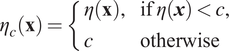 $$ {\eta}_c\left(\mathbf{x}\right)=\left\{\begin{array}{ll}\eta \left(\mathbf{x}\right),& \mathrm{if}\;\eta \left(\boldsymbol{x}\right)<c,\\ {}c& \mathrm{otherwise}\end{array}\right. $$
where $ \eta \left(\cdot \right) $
has been defined earlier. The distribution of
$ \eta \left(\cdot \right) $
has been defined earlier. The distribution of $ {\eta}_c\left(\mathbf{x}\right) $
at design points
$ {\eta}_c\left(\mathbf{x}\right) $
at design points $ \mathbf{x}=\left({\boldsymbol{x}}_c,{\boldsymbol{x}}_o\right) $
is then (Kyzyurova, Reference Kyzyurova2017):
$ \mathbf{x}=\left({\boldsymbol{x}}_c,{\boldsymbol{x}}_o\right) $
is then (Kyzyurova, Reference Kyzyurova2017):
 $$ {\displaystyle \begin{array}{l}\eta \left({\boldsymbol{x}}_o\right)\mid \boldsymbol{\beta}, {\sigma}^2,\boldsymbol{\theta}, \tau \sim \mathrm{N}\left({H}_o\boldsymbol{\beta}, {\sigma}^2{\Sigma}_o\right),\hskip1.5pt {\eta}_c\left({\boldsymbol{x}}_c\right)\mid \eta \left({\boldsymbol{x}}_o\right),\boldsymbol{\beta}, {\sigma}^2,\boldsymbol{\theta}, \tau \sim {\mathrm{TN}}_{\left(c,\infty \right)}\left({m}_c,{V}_c\right),\\ {}{m}_c={H}_c\boldsymbol{\beta} +{\Sigma}_{c,o}{\Sigma}_o^{-1}\left(\eta \left({\boldsymbol{x}}_{\mathbf{o}}\right)-{H}_o\boldsymbol{\beta} \right)\hskip1.5pt \mathrm{and}\hskip1.5pt {V}_c={\sigma}^2\left({\Sigma}_c-{\Sigma}_{c,o}{\Sigma}_o^{-1}{\Sigma}_{o,c}\right),\end{array}} $$
where $ {\mathrm{TN}}_{\left(c,\infty \right)} $
denotes a normal distribution truncated below
$ {\mathrm{TN}}_{\left(c,\infty \right)} $
denotes a normal distribution truncated below $ c $
. In (4),
$ c $
. In (4), $ {H}_o $
and
$ {H}_o $
and $ {\Sigma}_o $
are equivalent to
$ {\Sigma}_o $
are equivalent to $ {H}_x $
and
$ {H}_x $
and $ {\Sigma}_x $
as defined as in Section 3.1, here using the inputs
$ {\Sigma}_x $
as defined as in Section 3.1, here using the inputs $ {\boldsymbol{x}}_o $
. Similarly,
$ {\boldsymbol{x}}_o $
. Similarly, $ {H}_c $
is a matrix of regressors associated with
$ {H}_c $
is a matrix of regressors associated with $ {\boldsymbol{x}}_c $
, that is, its
$ {\boldsymbol{x}}_c $
, that is, its $ i $
th row is
$ i $
th row is $ h\left({\boldsymbol{x}}_{c,i}\right) $
, and
$ h\left({\boldsymbol{x}}_{c,i}\right) $
, and $ {\Sigma}_{c\left(i,j\right)}=C\left({\boldsymbol{x}}_{c,i},{\boldsymbol{x}}_{c,j},\boldsymbol{\theta} \right)+\tau \unicode{x1D540}\left(i,j\right) $
. Also,
$ {\Sigma}_{c\left(i,j\right)}=C\left({\boldsymbol{x}}_{c,i},{\boldsymbol{x}}_{c,j},\boldsymbol{\theta} \right)+\tau \unicode{x1D540}\left(i,j\right) $
. Also, $ {\Sigma}_{c,x\left(i,j\right)}=C\left({\boldsymbol{x}}_{c,i},{\boldsymbol{x}}_{o,j},\boldsymbol{\theta} \right) $
and
$ {\Sigma}_{c,x\left(i,j\right)}=C\left({\boldsymbol{x}}_{c,i},{\boldsymbol{x}}_{o,j},\boldsymbol{\theta} \right) $
and $ {\Sigma}_{o,c}={\Sigma}_{c,o}^T $
. To obtain truncated multivariate normal samples from Equation (4) (used later in a Gibbs sampler), we used the “TruncatedNormal” package in R (Botev and Belzile, Reference Botev and Belzile2020). The package uses a minimax tilting method for exact i.i.d. data simulation from the truncated multivariate normal distribution. More details can be found in Botev (Reference Botev2017).
$ {\Sigma}_{o,c}={\Sigma}_{c,o}^T $
. To obtain truncated multivariate normal samples from Equation (4) (used later in a Gibbs sampler), we used the “TruncatedNormal” package in R (Botev and Belzile, Reference Botev and Belzile2020). The package uses a minimax tilting method for exact i.i.d. data simulation from the truncated multivariate normal distribution. More details can be found in Botev (Reference Botev2017).
3.3. Bayesian inference and prediction
Inference for the GPE $ \eta \left(\cdot \right) $
and its parameters
$ \eta \left(\cdot \right) $
and its parameters $ \boldsymbol{\beta}, {\sigma}^2,\boldsymbol{\theta} $
and
$ \boldsymbol{\beta}, {\sigma}^2,\boldsymbol{\theta} $
and $ \tau $
above could be obtained by maximum likelihood using numerical optimization. While this easily produces point estimates, it is hard to take into account all sources of uncertainty (O’Hagan, Reference O’Hagan2006). Instead, we follow a Bayesian approach which can naturally incorporate parameter uncertainty, using MCMC (Brooks et al., Reference Brooks, Gelman, Jones and Meng2010) for inference. We used a Metropolis-within-Gibbs sampler whereby
$ \tau $
above could be obtained by maximum likelihood using numerical optimization. While this easily produces point estimates, it is hard to take into account all sources of uncertainty (O’Hagan, Reference O’Hagan2006). Instead, we follow a Bayesian approach which can naturally incorporate parameter uncertainty, using MCMC (Brooks et al., Reference Brooks, Gelman, Jones and Meng2010) for inference. We used a Metropolis-within-Gibbs sampler whereby $ \boldsymbol{\beta}, {\sigma}^2,\boldsymbol{\theta} $
and
$ \boldsymbol{\beta}, {\sigma}^2,\boldsymbol{\theta} $
and $ \tau $
were updated using Metropolis–Hastings steps and
$ \tau $
were updated using Metropolis–Hastings steps and $ {\boldsymbol{y}}_c $
was updated using a Gibbs step using Equation (4). Section 4.3 has more details regarding our application.
$ {\boldsymbol{y}}_c $
was updated using a Gibbs step using Equation (4). Section 4.3 has more details regarding our application.
Parameters inferred using MCMC can then be used for predicting the simulator output over a grid of inputs. Using a Bayesian predictive distribution (BPD) accounts for parameter uncertainty. One can sample from the marginal BPD for input $ \boldsymbol{v}=\left({v}_1,{v}_2,\dots, {v}_p\right) $
as follows. First, randomly select an iteration of the MCMC output and use the corresponding parameters. Second, use Equation (2) to sample from the GPE for input
$ \boldsymbol{v}=\left({v}_1,{v}_2,\dots, {v}_p\right) $
as follows. First, randomly select an iteration of the MCMC output and use the corresponding parameters. Second, use Equation (2) to sample from the GPE for input $ \boldsymbol{v} $
given the selected parameters (taking
$ \boldsymbol{v} $
given the selected parameters (taking $ \boldsymbol{x}=\left({\boldsymbol{x}}_o,{\boldsymbol{x}}_c\right) $
and
$ \boldsymbol{x}=\left({\boldsymbol{x}}_o,{\boldsymbol{x}}_c\right) $
and $ \boldsymbol{y}=\left({\boldsymbol{y}}_o,{\boldsymbol{y}}_c\right) $
where
$ \boldsymbol{y}=\left({\boldsymbol{y}}_o,{\boldsymbol{y}}_c\right) $
where $ {\boldsymbol{y}}_c $
is part of the MCMC output). Repeated sampling produces a Monte Carlo approximation to the marginal BPD at this location. This was used to produce Figure 3 and Supplementary Figures S2, S3, and S7.
$ {\boldsymbol{y}}_c $
is part of the MCMC output). Repeated sampling produces a Monte Carlo approximation to the marginal BPD at this location. This was used to produce Figure 3 and Supplementary Figures S2, S3, and S7.
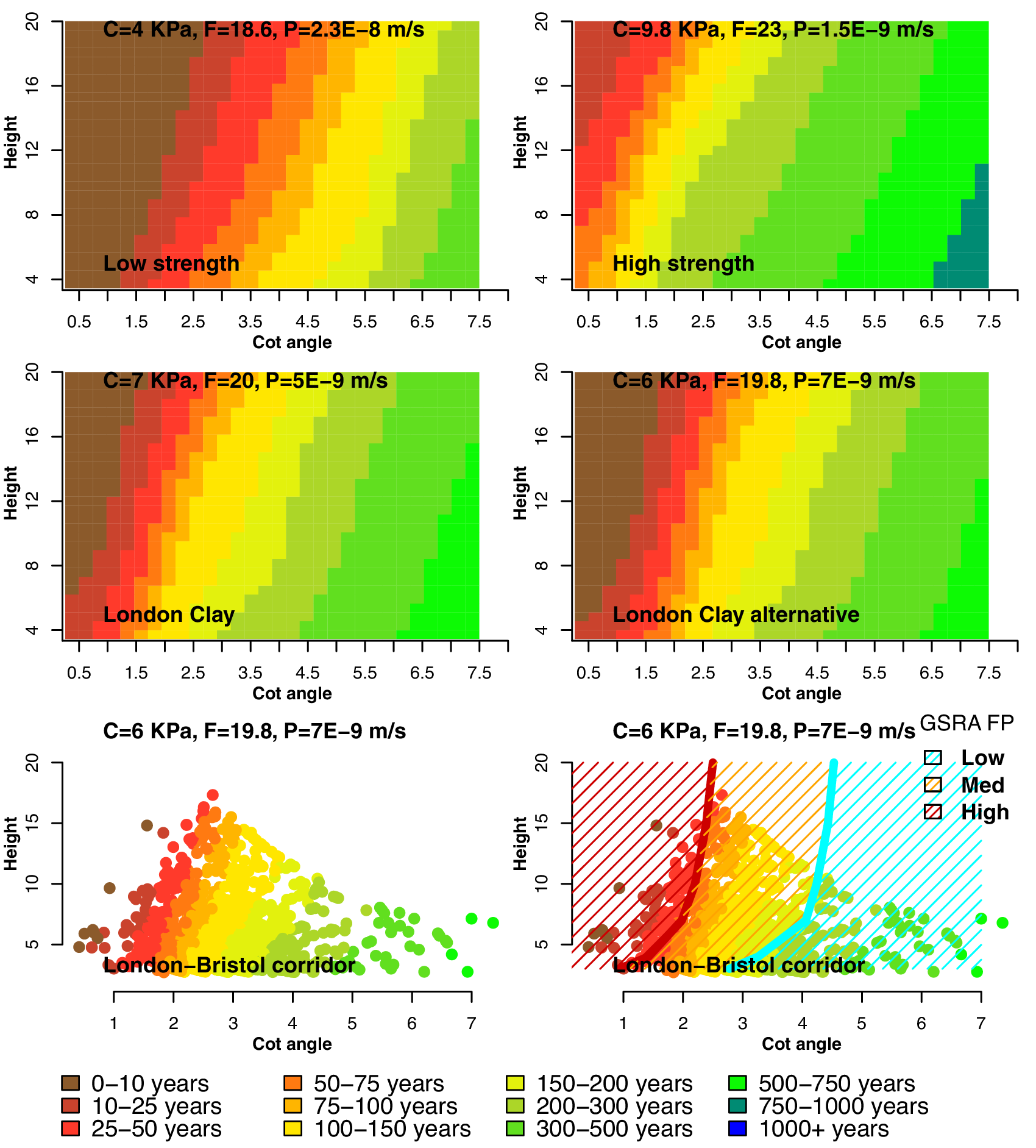
Figure 3. Expected time to failure for the GPE model. Cohesion kPa (C), friction angle (F), and permeability m/s (P) are fixed for every scenario and shown in the top left. The bottom-right plot illustrates the GSRA (Network Rail, 2017) failure potential (GSRA FP) contours. Posterior predictive variance maps are shown in Supplementary Figure S8.
3.4. Sensitivity analysis
It is often important to quantify the effect of different input variables on the response of a GPE. This can be obtained through sensitivity analysis (SA) (O’Hagan, Reference O’Hagan2006; Farah and Kottas, Reference Farah and Kottas2014). Sensitivity indices explain the proportion of variation in the mean response of the emulator because of an individual or a combination of input variable(s) (Gramacy, Reference Gramacy2020).
Assume that $ U $
represents the input density. For independent input variables
$ U $
represents the input density. For independent input variables $ {x}_i $
,
$ {x}_i $
, $ U(x)={\prod}_{i=1}^p{u}_i\left({x}_i\right) $
, where
$ U(x)={\prod}_{i=1}^p{u}_i\left({x}_i\right) $
, where $ {u}_i $
are the
$ {u}_i $
are the $ {x}_i $
marginal densities. The simplest form of sensitivity indices are the main effects (ME) (Gramacy, Reference Gramacy2020) of an explanatory variable
$ {x}_i $
marginal densities. The simplest form of sensitivity indices are the main effects (ME) (Gramacy, Reference Gramacy2020) of an explanatory variable $ {x}_i,i=1,2,\dots, p $
:
$ {x}_i,i=1,2,\dots, p $
:
 $$ me\left({x}_i\right)\equiv {E}_{U_{-i}}\left\{\eta |{x}_i\right\}=\int {\int}_{-{\chi}_{-i}}\eta p\left(\eta |{x}_1,{x}_2,\dots, {x}_p\right)\cdot {u}_{-i}\left({x}_{-i}\right){dx}_{-i} d\eta . $$
Here, $ {u}_{-j}={\prod}_{i\ne j}{u}_i\left({x}_i\right) $
, and
$ {u}_{-j}={\prod}_{i\ne j}{u}_i\left({x}_i\right) $
, and $ {\chi}_{-i} $
and
$ {\chi}_{-i} $
and $ {x}_{-i} $
are defined similarly (Gramacy, Reference Gramacy2020). The formalism (5) deterministically varies
$ {x}_{-i} $
are defined similarly (Gramacy, Reference Gramacy2020). The formalism (5) deterministically varies $ {x}_i $
while averaging over the input densities
$ {x}_i $
while averaging over the input densities $ {U}_{-i} $
, assuming that all inputs are uncorrelated. In other words,
$ {U}_{-i} $
, assuming that all inputs are uncorrelated. In other words, $ me\left({x}_i\right) $
is the expected value of the response given
$ me\left({x}_i\right) $
is the expected value of the response given $ {x}_i $
while averaging over
$ {x}_i $
while averaging over $ {x}_{-i} $
. The distributions of the main effects are calculated by calculating the expectation in Equation (5) at every MCMC sample of the
$ {x}_{-i} $
. The distributions of the main effects are calculated by calculating the expectation in Equation (5) at every MCMC sample of the $ \eta \left(\cdot \right) $
posterior distributions.
$ \eta \left(\cdot \right) $
posterior distributions.
In our application, we also perform a fully Bayesian SA using first-order and total sensitivity indices following the method in Farah and Kottas (Reference Farah and Kottas2014) and Gramacy (Reference Gramacy2020): the derivation of the following formalisms can be found therein. The first-order sensitivity index $ {S}_{1,i},i=1,2,\dots, p $
evaluates the fractional contribution of the
$ {S}_{1,i},i=1,2,\dots, p $
evaluates the fractional contribution of the $ {x}_i $
input variable to the variance of the output (Farah and Kottas, Reference Farah and Kottas2014):
$ {x}_i $
input variable to the variance of the output (Farah and Kottas, Reference Farah and Kottas2014):
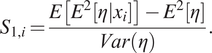 $$ {S}_{1,i}=\frac{E\left[{E}^2\left[\eta |{x}_i\right]\right]-{E}^2\left[\eta \right]}{Var\left(\eta \right)}. $$
In other words, $ {S}_{1.i} $
is the response sensitivity to main variable effects (Gramacy, Reference Gramacy2020). The total sensitivity index (Homma and Saltelli, Reference Homma and Saltelli1996; Farah and Kottas, Reference Farah and Kottas2014)
$ {S}_{1.i} $
is the response sensitivity to main variable effects (Gramacy, Reference Gramacy2020). The total sensitivity index (Homma and Saltelli, Reference Homma and Saltelli1996; Farah and Kottas, Reference Farah and Kottas2014) $ {S}_{T,i} $
is a measure of the entire influence attributable to a given variable (Gramacy, Reference Gramacy2020):
$ {S}_{T,i} $
is a measure of the entire influence attributable to a given variable (Gramacy, Reference Gramacy2020):
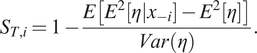 $$ {S}_{T,i}=1-\frac{E\left[{E}^2\left[\eta |{x}_{-i}\right]-{E}^2\left[\eta \right]\right]}{Var\left(\eta \right)}. $$
A large difference between the distributions of $ {S}_{1,i} $
and
$ {S}_{1,i} $
and $ {S}_{T,i} $
would indicate that the interactions between the
$ {S}_{T,i} $
would indicate that the interactions between the $ {x}_i $
and the remaining input variables are important to explaining the output variation (Farah and Kottas, Reference Farah and Kottas2014). The posterior distributions of the sensitivity indices can be sampled by computing the expectations in Equations (6) and (7) at every MCMC sample of the emulator parameters (Farah and Kottas, Reference Farah and Kottas2014).
$ {x}_i $
and the remaining input variables are important to explaining the output variation (Farah and Kottas, Reference Farah and Kottas2014). The posterior distributions of the sensitivity indices can be sampled by computing the expectations in Equations (6) and (7) at every MCMC sample of the emulator parameters (Farah and Kottas, Reference Farah and Kottas2014).
3.5. Experimental design
The reliability of the emulator very strongly depends on the experimental design (Busby, Reference Busby2009), that is, the choice of input variables. Space-filling designs aim to spread out the input variables and produce a diversity of data once responses have been observed (Gramacy, Reference Gramacy2020). We focus on a particular space-filling approach: Latin hypercube designs (LHD). Here each of the $ p $
input variables are divided into
$ p $
input variables are divided into $ N $
equally sized intervals and one point is selected randomly per interval in each dimension (Santner, Reference Santner2018; Gramacy, Reference Gramacy2020).
$ N $
equally sized intervals and one point is selected randomly per interval in each dimension (Santner, Reference Santner2018; Gramacy, Reference Gramacy2020).
Although LHDs are space-filling in each of the input coordinates, however, they are not necessarily space filling in the $ p $
-dimensional hypercube space (Dette and Pepelyshev, Reference Dette and Pepelyshev2021). An alternative approach is to search for a design optimizing the maximin criterion: maximizing the minimum distance between pairs of points (Santner, Reference Santner2018; Gramacy, Reference Gramacy2020). We used a hybrid maximin LHD approach in which five LHDs are generated, and the optimal maximin choice is selected. This was implemented using the package “pyDOE” (Baudin et al., Reference Baudin, Christopoulou, Colette and Martinez2012) in Python.
$ p $
-dimensional hypercube space (Dette and Pepelyshev, Reference Dette and Pepelyshev2021). An alternative approach is to search for a design optimizing the maximin criterion: maximizing the minimum distance between pairs of points (Santner, Reference Santner2018; Gramacy, Reference Gramacy2020). We used a hybrid maximin LHD approach in which five LHDs are generated, and the optimal maximin choice is selected. This was implemented using the package “pyDOE” (Baudin et al., Reference Baudin, Christopoulou, Colette and Martinez2012) in Python.
4. Application Methods
4.1. Model, priors, and design
We deployed a GP emulator for GM experiments of rail cut slope stability. We emulated the output variable of time to failure (TTF), that is, the time to reaching the slope’s ultimate failure state. As input variables, we used slope height, angle cotangent, (effective) peak cohesion, (effective) peak friction angle, and permeability (hydraulic conductivity). In our earlier notation, these variables are, respectively, $ {h}_s,\cot {\theta}_s,{c}_p^{\prime },{\phi}_p^{\prime },{k}_1^w $
. However, for ease of reference, we refer to these as
$ {h}_s,\cot {\theta}_s,{c}_p^{\prime },{\phi}_p^{\prime },{k}_1^w $
. However, for ease of reference, we refer to these as $ {x}_1,{x}_2,\dots, {x}_5 $
below.
$ {x}_1,{x}_2,\dots, {x}_5 $
below.
We used LHD to create 76 vectors of input variables to use as the training suite of the GM experiments. This was based on a four-dimensional design, with the first dimension corresponding to a combination of height and angle cotangent which we refer to as geometry; see Supplementary Figure S1 for details. Based on exploratory analysis, detailed in Section 4.2, we used the full linear form of the regressor function $ h\left(\boldsymbol{x}\right) $
, including an intercept,
$ h\left(\boldsymbol{x}\right) $
, including an intercept, $ h\left(\boldsymbol{x}\right)=\left(1,{x}_1,{x}_2,\dots, {x}_5\right) $
. Thus, our mean function was
$ h\left(\boldsymbol{x}\right)=\left(1,{x}_1,{x}_2,\dots, {x}_5\right) $
. Thus, our mean function was $ m\left(\boldsymbol{x}\right)={\beta}_0+{\sum}_{i=1}^5{\beta}_i{x}_i $
.
$ m\left(\boldsymbol{x}\right)={\beta}_0+{\sum}_{i=1}^5{\beta}_i{x}_i $
.
The prior distributions for $ \beta, \theta $
and
$ \beta, \theta $
and $ {\sigma}^2 $
were chosen to reflect beliefs of our geotechnical and statistical experts about
$ {\sigma}^2 $
were chosen to reflect beliefs of our geotechnical and statistical experts about $ \eta \left(\cdot \right) $
:
$ \eta \left(\cdot \right) $
:
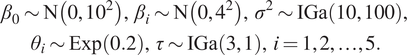 $$ {\displaystyle \begin{array}{c}{\beta}_0\sim \mathrm{N}\left(0,{10}^2\right),\hskip2pt {\beta}_i\sim \mathrm{N}\left(0,{4}^2\right),\hskip2pt {\sigma}^2\sim \mathrm{IGa}\left(\mathrm{10,100}\right),\\ {}{\theta}_i\sim \mathrm{Exp}(0.2),\hskip2pt \tau \sim \mathrm{IGa}\left(3,1\right),\hskip2pt i=1,2,\dots, 5.\end{array}} $$
Also note that it is important to select informative priors for the covariance function parameters, otherwise identifiability issues are common (see, e.g., Zhang, Reference Zhang2004).
4.2. Modeling and tuning choices
4.2.1. Alternative regressor choices
We compared our full linear choice of $ h\left(\boldsymbol{x}\right) $
to other choices, in particular,
$ h\left(\boldsymbol{x}\right) $
to other choices, in particular, $ h\left(\boldsymbol{x}\right)=0 $
(zero mean) and
$ h\left(\boldsymbol{x}\right)=0 $
(zero mean) and $ h\left(\boldsymbol{x}\right)=1 $
(constant mean). Note that in the geostatistical literature, the full linear and constant mean forms of
$ h\left(\boldsymbol{x}\right)=1 $
(constant mean). Note that in the geostatistical literature, the full linear and constant mean forms of $ h\left(\boldsymbol{x}\right) $
correspond to universal and simple forms of kriging (Oliver and Webster, Reference Oliver and Webster2015). Supplementary Figure S2 shows results comparing choices of
$ h\left(\boldsymbol{x}\right) $
correspond to universal and simple forms of kriging (Oliver and Webster, Reference Oliver and Webster2015). Supplementary Figure S2 shows results comparing choices of $ h\left(\boldsymbol{x}\right) $
. It illustrates that the full linear form of
$ h\left(\boldsymbol{x}\right) $
. It illustrates that the full linear form of $ h\left(\boldsymbol{x}\right) $
appears most appropriate, as the resulting TTF contours are near-linear and are consistent with the literature (Ellis and O’Brien, Reference Ellis and O’Brien2007; Gao et al., Reference Gao, Wu and Zhang2015). Using only a constant mean term for
$ h\left(\boldsymbol{x}\right) $
appears most appropriate, as the resulting TTF contours are near-linear and are consistent with the literature (Ellis and O’Brien, Reference Ellis and O’Brien2007; Gao et al., Reference Gao, Wu and Zhang2015). Using only a constant mean term for $ h\left(\boldsymbol{x}\right) $
led to nonmonotonic dependence of TTF on slope angle, which was deemed to be unrealistic. The full linear form also allows both the mean and the covariance functions to contribute to explaining variation in the relationship between the input and response, as opposed to the covariance function only when using a constant or zero mean.
$ h\left(\boldsymbol{x}\right) $
led to nonmonotonic dependence of TTF on slope angle, which was deemed to be unrealistic. The full linear form also allows both the mean and the covariance functions to contribute to explaining variation in the relationship between the input and response, as opposed to the covariance function only when using a constant or zero mean.
4.2.2. Transformation of response and choice of kernel
Various transformations of the TTF were considered to avoid predicting negative values and to minimize prediction errors. The discussion and illustration of their predictive properties for a set of validation runs are shown in section “Output transformation validation” and Supplementary Figure S3. Supplementary Figure S3 illustrates the goodness of predictions for the different transformations by plotting them against the observed times to failure. Square root transformation appears to give the highest agreement with the observed TTFs, illustrated by the lowest mean square error. Additionally, the $ {C}_M\left(\boldsymbol{x},{\boldsymbol{x}}^{\prime },\boldsymbol{\theta}, 5/2\right) $
(abbreviated as
$ {C}_M\left(\boldsymbol{x},{\boldsymbol{x}}^{\prime },\boldsymbol{\theta}, 5/2\right) $
(abbreviated as $ {C}_{M,5/2} $
) correlation function gave the optimal
$ {C}_{M,5/2} $
) correlation function gave the optimal $ {R}^2 $
and MSE. The cube root transformation also appears plausible. However, it over-predicts the TTF in its upper distribution tail. Therefore, the square root transformation of TTF and
$ {R}^2 $
and MSE. The cube root transformation also appears plausible. However, it over-predicts the TTF in its upper distribution tail. Therefore, the square root transformation of TTF and $ {C}_{M,5/2} $
was used for this study.
$ {C}_{M,5/2} $
was used for this study.
4.3. MCMC details
The regressor coefficients $ {\beta}_0 $
and
$ {\beta}_0 $
and $ {\beta}_4 $
were updated jointly using a multivariate normal proposal distribution centered at the current chain value. The variance matrix of the proposal distribution was set to approximate the posterior correlation that was observed in a pilot run. Component-wise updates were used for
$ {\beta}_4 $
were updated jointly using a multivariate normal proposal distribution centered at the current chain value. The variance matrix of the proposal distribution was set to approximate the posterior correlation that was observed in a pilot run. Component-wise updates were used for $ {\beta}_1,{\beta}_2,{\beta}_3 $
, and
$ {\beta}_1,{\beta}_2,{\beta}_3 $
, and $ {\beta}_5 $
, using an adaptive proposal variance following the procedure by Xiang and Neal (Reference Xiang and Neal2014). The parameters
$ {\beta}_5 $
, using an adaptive proposal variance following the procedure by Xiang and Neal (Reference Xiang and Neal2014). The parameters $ {\sigma}^2,\tau $
and
$ {\sigma}^2,\tau $
and $ {\theta}_i,i=1,2,\dots, 5 $
were updated using a log-normal proposal distribution centered at the natural logarithm of the current chain value. The proposal variances of
$ {\theta}_i,i=1,2,\dots, 5 $
were updated using a log-normal proposal distribution centered at the natural logarithm of the current chain value. The proposal variances of $ {\sigma}^2,{\theta}_i $
and
$ {\sigma}^2,{\theta}_i $
and $ \tau $
were also tuned using the above method. The censored observations
$ \tau $
were also tuned using the above method. The censored observations $ \eta \left({\boldsymbol{x}}_c\right) $
were updated using a Gibbs step following Equation (4).
$ \eta \left({\boldsymbol{x}}_c\right) $
were updated using a Gibbs step following Equation (4).
The chain burn-in and variance adaptive period was $ {10}^5 $
iterations which were discarded and the scheme was then run for a further
$ {10}^5 $
iterations which were discarded and the scheme was then run for a further $ 2\times {10}^5 $
iterations. Supplementary Figure S4 illustrates the trace plots of the MCMC draws. Good mixing can be observed for all parameters, especially the censored observations. Supplementary Figure S5 illustrates effective sample sizes (ESSs) for the three correlation functions, which is a diagnostic for posterior autocorrelation (Brooks et al., Reference Brooks, Gelman, Jones and Meng2010). All of the ESSs are above 3,000 with censored observations having the highest values.
$ 2\times {10}^5 $
iterations. Supplementary Figure S4 illustrates the trace plots of the MCMC draws. Good mixing can be observed for all parameters, especially the censored observations. Supplementary Figure S5 illustrates effective sample sizes (ESSs) for the three correlation functions, which is a diagnostic for posterior autocorrelation (Brooks et al., Reference Brooks, Gelman, Jones and Meng2010). All of the ESSs are above 3,000 with censored observations having the highest values.
5. Application Results
5.1. Parameter inference
Figure 1 illustrates the posterior densities of the GPE parameters, all of which appear unimodal. Posterior density plots for all of the censored values can be found in Supplementary Figure S6. For most parameters, the posterior variance is significantly reduced compared with the prior distribution. This is especially the case for most $ \boldsymbol{\beta} $
coefficients and the censored values. Most of the posterior densities of the censored observations (Supplementary Figure S6) also show a decrease in variance compared with that of their prior distributions. The larger posterior variances can be observed for the observations with larger posterior means, for example,
$ \boldsymbol{\beta} $
coefficients and the censored values. Most of the posterior densities of the censored observations (Supplementary Figure S6) also show a decrease in variance compared with that of their prior distributions. The larger posterior variances can be observed for the observations with larger posterior means, for example, $ {y}_{c,1} $
and
$ {y}_{c,1} $
and $ {y}_{c,3} $
, as those estimates have the largest distance to the training data. Conversely, the uncertainty around the posterior estimations of, for example,
$ {y}_{c,3} $
, as those estimates have the largest distance to the training data. Conversely, the uncertainty around the posterior estimations of, for example, $ {y}_{c,53} $
and
$ {y}_{c,53} $
and $ {y}_{c,68} $
is very small. There is relatively little info about
$ {y}_{c,68} $
is very small. There is relatively little info about $ \boldsymbol{\theta} $
in the data; however, their posterior distributions are relatively close to their priors compared with those of
$ \boldsymbol{\theta} $
in the data; however, their posterior distributions are relatively close to their priors compared with those of $ \boldsymbol{\beta} $
.
$ \boldsymbol{\beta} $
.
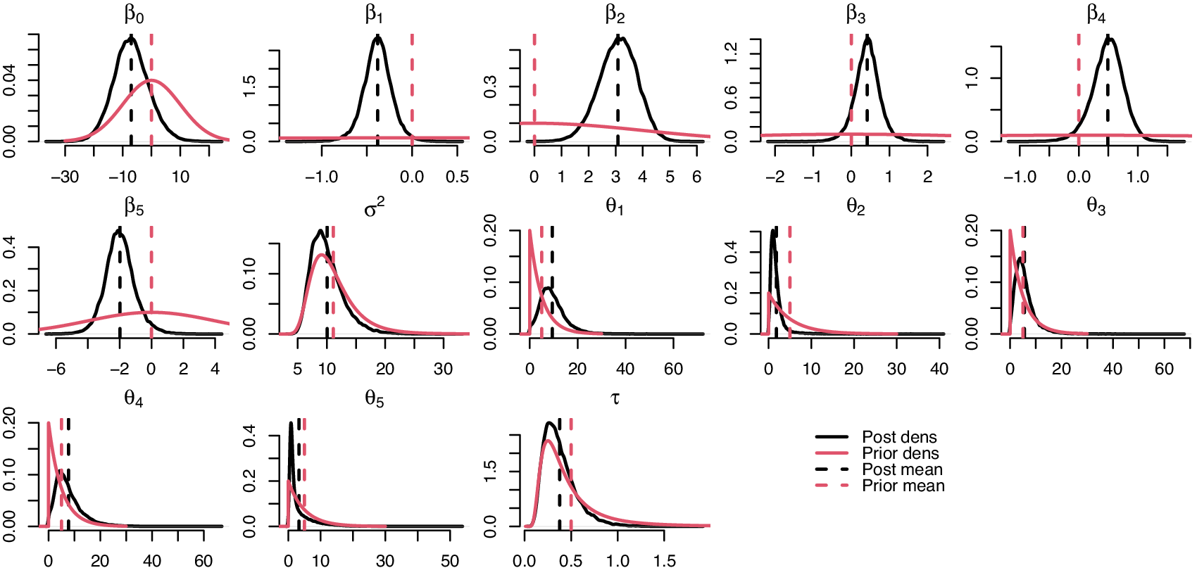
Figure 1. Density plots of the posterior draws of the GPE model. Density plots of the $ {\boldsymbol{y}}_c $
posterior distributions are in Supplementary Figure S6.
$ {\boldsymbol{y}}_c $
posterior distributions are in Supplementary Figure S6.
Supplementary Figure S7 illustrates the posterior marginal distributions of the TTF versus each of the input variables. The majority of the data is captured in the 95% confidence interval bands. While all of the relations have a trend, slope angle cotangent appears to have the strongest relation with the TTF.
5.2. Sensitivity analysis
Figure 2a illustrates a main effects sensitivity analysis of the input variables, which are equivalent to the mean trends in Supplementary Figure S7. All of the main effects are monotonic, and the most influential variable appears to be slope angle cotangent, in this case because of the steepest gradient. Cohesion and friction angle have very similar main effects as they soften at the same rate as a function of plastic strain (e.g., Labuz and Zang, Reference Labuz and Zang2012).

Figure 2. Sensitivity analysis of the GPE. Plot (a) illustrates the main effects sensitivity analysis corresponding to Equation 5, and plot (b) illustrates first-order and total sensitivity indices corresponding to Equations 6 and 7. Slope angle cotangent, cohesion, friction angle, and permeability are abbreviated “Cot”, “Coh”, “Fric”, and “Perm”. In plot (a), square root of time to failure is abbreviated “Sqrt TTF”.
Figure 2b illustrates the first-order and total sensitivity index distributions. Again, angle cotangent has the greatest contribution to the variability in TTF, followed by height. Cohesion, friction angle, and permeability explain a similar proportion of the TTF variability. All of the input variables have similar distributions of the first-order and total sensitivity indices, indicating an absence of strong interaction effects (Farah and Kottas, Reference Farah and Kottas2014).
5.3. TTF posterior predictive maps
Plots of TTF versus slope geometry can be very informative in illustrating deterioration given fixed soil strength and permeability. Plots of TTF versus slope geometry allow infrastructure owners and designers to estimate likely design life of geotechnical infrastructure where previously this was not possible. Figure 3 illustrates the distribution of TTF for slope height and angle in four soil strength scenarios (cohesion, friction angle, and permeability values are shown in the legend). All of the negative predicted values were set to zero. Supplementary Figure S8 illustrates equivalent maps of posterior predictive variance. Low- and high-strength soils reflect the range of shear strengths for over-consolidated high-plasticity clays based on laboratory and filed data for London Clay strength and permeability (Bromhead and Dixon, Reference Bromhead and Dixon1986; Potts et al., Reference Potts, Kovacevic and Vaughan1997).
The change in TTF is approximately linear with respect to geometry, and appears most sensitive to changes in the slope angle. This is consistent with our sensitivity analysis and failure profiles reported earlier in the literature (Ellis and O’Brien, Reference Ellis and O’Brien2007; Gao et al., Reference Gao, Wu and Zhang2015). For the low-strength soil example, a significant proportion of slope geometries fail in less than 10 years. Fortunately, the scenario is unlikely be representative of average in situ peak strength conditions for the whole soil mass (e.g., Kovacevic et al., Reference Kovacevic, Hight and Potts2007), especially where vegetation roots can influence soil strength at the near surface (Woodman et al., Reference Woodman, Smethurst, Roose, Powrie, Meijer, Knappett and Dias2020). For London Clay examples, the TTF contours are consistent with the literature (Ellis and O’Brien, Reference Ellis and O’Brien2007; Gao et al., Reference Gao, Wu and Zhang2015). The plots in the lower panel of Figure 3 illustrating TTF for the cuttings in the London–Bristol corridor assumes strength and permeability in agreement with published results (Hight et al., Reference Hight, McMillan, Powell, Jardine and Allenou2003; Dixon et al., Reference Dixon, Crosby, Stirling, Hughes, Smethurst, Briggs, Hughes, Gunn, Hobbs, Loveridge, Glendinning, Dijkstra and Hudson2019). Note that the training data do not cover the upper ranges of slope height and angle (i.e., upper triangle of the plots), thus the TTF predictions made in that region are an extrapolation.
Supplementary Figure S8 illustrates that the posterior variance is minimized for London Clay-type soils which are away from the boundaries of our Latin Hypercube design. Therefore, extrapolating further away from the experimental data leads to a rapid increase in posterior variance which is undesirable. In conditions of low data availability, it would be advisable to avoid construction of slopes which are too steep or too shallow. Also, it would be advisable to perform another numerical experiment and emulation for materials which are toward or outside the boundary of our design, for example, medium-plasticity clays.
5.3.1. Comparison to previous work
Our results in Figure 3 are consistent with those of the Global Stability and Resilience Appraisal (GSRA) performed by Mott Macdonald and Network Rail (Network Rail, 2017; Abbott, Reference Abbott2018). They derived contours of vulnerability to deep-seated rotational failure for soils with different plasticities. The bottom plots illustrate the cutting slope geometry data in the London–Bristol corridor that are built in London Clay-type soil (data provided by Mott MacDonald and Network Rail). The bottom-right plot in Figure 3 overlays the vulnerability contours for cuttings in cohesive, high-plasticity soils over the TTF predictions for cuttings in the London–Bristol corridor. The high GSRA failure potential (FP)corresponds to TTFs of 50 years or less. The low FP corresponds to TTFs of 150 years and above. At low slope heights ( $ <8 $
m), the vulnerability contours are determined by a combination of height and angle. For other heights, they are almost entirely determined by the angle. In our predictions, the relation between TTF and slope geometry is more linear, although the gradient is steeper in the slope angle direction, which is consistent with our sensitivity analysis.
$ <8 $
m), the vulnerability contours are determined by a combination of height and angle. For other heights, they are almost entirely determined by the angle. In our predictions, the relation between TTF and slope geometry is more linear, although the gradient is steeper in the slope angle direction, which is consistent with our sensitivity analysis.
6. Conclusion
We have used GP emulation to produce a surrogate for the cutting slope stability GM. The high computational expense of the latter renders it impractical to evaluate for the number of experiments that is required for understanding the input–output relationships. Latin hypercube sampling was used to design an optimally space-filling experiment to train the emulator. Bayesian inference and MCMC simulation were used to estimate the GPE parameters. For a number of experiments, the ultimate failure state was not achieved during the 184 years of experimental time. For such models, the TTF was unobserved and was later also estimated using MCMC. The trained GPE was then used to produce TTF maps illustrating the relationship between slope geometry and FP. The computational expense involved in producing such inference is on the order of hours, which makes the GPE a highly attractive tool that can be used in real-time for rapid characterization of slope stability and deterioration. For instance, every plot in Figure 3 has 900 points and takes 3–4 hr to produce once the emulator has been trained, and its computation could be easily parallelized if necessary. Conversely, 900 runs of the GM simulator would take years of CPU time to evaluate, thus would be unfeasible. As the TTF maps can be provided for any combination of input parameters, the emulator has an outstanding computational advantage over the GM simulator and has a great potential to inform infrastructure slope design and maintenance in engineering practice. Future work in developing the emulator includes incorporating weather and climate change variables, for example, discrete extreme rainfall events along with the changing patterns and magnitude of seasonal weather thought likely to occur because of a changing future climate.
Acknowledgment
The authors gratefully acknowledge the data provided by Dr. Chris Power of Mott MacDonald and Mr. Simon Abbott of Network Rail.
Funding Statement
The work presented is an output of the collaborative research project iSMART (grant number EP/K027050/1) and the program grant ACHILLES (grant number EP/R034575/1) funded by the U.K. Engineering and Physical Sciences Research Council (EPSRC).
Competing Interests
The authors declare no competing interests exist.
Data Availability Statement
The data that support the findings of this study are openly available in the repository Data for emulating computer experiments of infrastructure slope stability using Gaussian processes and Bayesian inference at https://doi.org/10.25405/data.ncl.14331314.v2. The corresponding code is available at https://doi.org/10.25405/data.ncl.14447670.v2.
Author Contributions
Conceptualization, D.J.W., P.H., M.R., S.G.; Data curation, P.H., D.J.W.; Formal analysis, A.S., P.H., D.P., D.J.W.; Funding acquisition, S.G.; Investigation, A.S., D.P., D.J.W.; Methodology, A.S., D.J.W., D.P., P.H., M.R.; Project administration, D.J.W., S.G.; Software, A.S., P.H., D.P., M.R., D.J.W.; Supervision, D.J.W., D.P., M.R., S.G.; Writing—original draft, A.S., P.H., D.P., D.J.W.; Writing—review and editing, A.S., P.H., D.P., M.R., S.G., D.J.W. All authors approved the final submitted draft.
Supplementary Materials
To view supplementary material for this article, please visit http://dx.doi.org/10.1017/dce.2021.14.


 Open access
Comments
No Comments have been published for this article.