


Impact Statement
Bayesian inference is increasingly discussed to identify the constitutive models’ parameters of soft tissue. However, sometimes the obtained parameters cannot predict the behavior of soft tissues. Therefore, in this work, the effect of incorporating “Model uncertainty” to reduce the mismatch between reality and model prediction has been explored.
1. Introduction
Constitutive models of soft tissues are crucial for computer-aided surgery, surgical training simulators, functional tissue engineering, and traumatic brain injury simulations (Humphrey, Reference Humphrey2003; Madireddy et al., Reference Madireddy, Sista and Vemaganti2015; Hauseux et al., Reference Hauseux, Hale, Cotin and Bordas2018; Bui et al., Reference Bui, Tomar and Bordas2019; Duprez et al., Reference Duprez, Bordas, Bucki, Bui, Chouly, Lleras, Lobos, Lozinski, Rohan and Tomar2020; Magliulo et al., Reference Magliulo, Lengiewicz, Zilian and Beex2020). Although several sophisticated constitutive models for soft tissues were proposed (Courtney et al., Reference Courtney, Sacks, Stankus, Guan and Wagner2006; Guo et al., Reference Guo, Peng and Moran2006), soft tissues are still often described using incompressible hyperelasticity. The simplicity of incompressible hyperelasticity has the advantage that few parameters need to be identified. The soft tissue models in this contribution are limited to incompressible hyperelasticity.
Parameter values of a soft tissue model identified during surgery may not be accurate, because the experimental data are sparse and affected by a substantial amount of measurement noise (due to the limitations of the type of observations and the sampling frequency of the observations). The uncertainties of the parameter values are, therefore, important to consider. Although conventional probabilistic identification frameworks can identify parameter uncertainties, they are traditionally not formulated to account for the fact that the model itself is limited to describe the data. To overcome this deficiency, model uncertainty can be incorporated in probabilistic identification frameworks.
Model uncertainty can be defined as the uncertainty due to the inability of a model to describe observations of the real world. Model uncertainty comes into play if a discrepancy between the model and the experimental data is present that cannot be explained by the noise in the data. A well-accepted approach to include the uncertainty of models in probabilistic identification settings was presented by Kennedy and O’Hagan (KOH) (Kennedy and O’Hagan, Reference Kennedy and O’Hagan2001). This “KOH” framework was, for instance, employed in (Arhonditsis et al., Reference Arhonditsis, Papantou, Zhang, Perhar, Massos and Shi2008; Higdon et al., Reference Higdon, Gattiker, Williams and Rightley2008; McFarland and Mahadevan, Reference McFarland and Mahadevan2008; Sankararaman et al., Reference Sankararaman, Ling, Shantz and Mahadevan2011; Arendt et al., Reference Arendt, Apley and Chen2012).
In the present work, we develop a KOH framework (able to treat both the uncertainty of the data and the uncertainty of the model) to identify uncertainties of the parameters of incompressible hyperelasticity. The aim is to investigate how different formulations of model uncertainty influence the identified parameter uncertainties. For this purpose, different model uncertainty formulations have been considered. These formulations range from uninformative to probabilistically more advanced ones, and from input-independent forms to formulations based on more advanced incompressible hyperelasticity. In this contribution, we consider synthetic data, so that we can make a quantitative comparison with the reference input. As this study is exploratory, we limit ourselves to tensile and compression data for which the model responses can be described by closed-form expressions.
1.1. Bayesian updating and its application in solid mechanics
Parameter identification is still largely performed in deterministic settings such as the method of least squares (Loh and Das, Reference Loh and Das1986; Wu and Lee, Reference Wu and Lee2006; Ortiz et al., Reference Ortiz, Banks, Castillo-Chávez, Chowell and Wang2011; Beex, Reference Beex2019; Loew et al., Reference Loew, Peters and Beex2020). The result of a deterministic identification procedure, such as least squares, is a single set of parameter values. This set is the most probable set of parameter values, assuming, for instance, that no discrepancy between model and measurements exists and that the noise is symmetrically distributed.
Probabilistic identification approaches aim to identify not only the most probable set of parameter values, but all sets of parameter values that may have produced the measured data. In other words, they aim to determine the probability of each set of parameter values. This is accomplished by identifying a probability density function (PDF) in terms of the model parameters. Instead of identifying material parameters, a PDF must be evaluated.
One probabilistic identification approach is Bayesian inference (BI), which is based on Bayes’ theorem. In BI, an initial PDF in terms of the constitutive parameters must be defined by the user. This initial PDF incorporates all a priori knowledge. This a priori knowledge can be relatively uninformative, for example, by stating that Young’s modulus cannot be negative, but it can also be more informative. For instance, if one knows that a cortical bone is considered, Young’s modulus is probably between 15 and 25 GPa.
In BI, the initial PDF (i.e., the prior) is updated by inferring the experimental data. This commonly entails that the noise distribution must be identified beforehand (Rappel et al., Reference Rappel, Beex, Hale, Noels and Bordas2020). However, the parameters of the noise distribution may also be treated as parameters that are to be simultaneously identified with the model parameters.
The final PDF that results from BI is called the posterior and is often so complex that the associated cumulative distribution function cannot be analytically expressed—entailing that sets of constitutive parameters cannot be randomly generated from the posterior. In those cases, the posterior is typically explored by seeding numerous samples and evaluating the PDF for each sample. Several numerical frameworks have been proposed in the past to limit the number of necessary samples (in order to decrease the computational cost of the numerical sampling). Well-known examples are Markov chain Monte Carlo techniques (Higdon et al., Reference Higdon, Lee and Bi2002; Wang and Zabaras, Reference Wang and Zabaras2004; Risholm et al., Reference Risholm, Janoos, Norton, Golby and Wells2013; Lan et al., Reference Lan, Bui-Thanh, Christie and Girolami2016) and hybrid Monte Carlo (HMC) methods (Beskos et al., Reference Beskos, Pillai, Roberts, Sanz-Serna and Stuart2013; Betancourt, Reference Betancourt2017).
One of the earlier works in which BI is exploited to identify parameter uncertainties in computational mechanics is that of Isenberg (Isenberg, Reference Isenberg1979), in which it was used to identify elastic parameters in 1979. In other works, the framework was employed to identify elastic material parameters based on dynamic responses (Alvin, Reference Alvin1997; Beck and Katafygiotis, Reference Beck and Katafygiotis1998; Marwala and Sibisi, Reference Marwala and Sibisi2005; Mohamedou et al., Reference Mohamedou, Zulueta, Chung, Rappel, Beex, Adam, Arriaga, Major, Wu and Noels2019). BI was also used to identify the elastic constants of composites (Lai and Ip, Reference Lai and Ip1996; Daghia et al., Reference Daghia, de Miranda, Ubertini and Viola2007; Nichols et al., Reference Nichols, Link, Murphy and Olson2010; Gogu et al., Reference Gogu, Yin, Haftka, Ifju, Molimard, Riche and Vautrin2013). Spatially varying elastic parameters were, furthermore, identified using BI by Koutsourelakis (Reference Koutsourelakis2012) and Hussein et al. (Reference Hussein, Wu, Noels and Beex2019). The Bayesian paradigm was also used for the identification of parameter uncertainties of constitutive models (Rappel et al., Reference Rappel, Beex and Bordas2018; Rappel et al., Reference Rappel, Beex, Noels and Bordas2019; Rappel and Beex, Reference Rappel and Beex2019; Teferra and Brewick, Reference Teferra and Brewick2019).
Two works have previously applied BI for the parameter identification of hyperelastic models (Madireddy et al., Reference Madireddy, Sista and Vemaganti2015; Madireddy et al., Reference Madireddy, Sista and Vemaganti2016). Madireddy et al. (Reference Madireddy, Sista and Vemaganti2015) considered three hyperelastic models for soft tissues and investigated the effect of the uncertainty on a quantity of interest. On the other hand, Ritto and Nunes (Reference Ritto and Nunes2015) exploited BI not only to identify parameter distributions, but also to select which hyperelastic model is most suited.
The difference between our contribution and the works of Madireddy et al. (Reference Madireddy, Sista and Vemaganti2015) and Ritto and Nunes is that we aim to investigate how the incorporation of different forms of model uncertainty affects the identified material parameter distributions. The reason that model uncertainty is relevant is that although probabilistic identification approaches identify the probability of all (meaningful) sets of material parameters (instead of only the most probable set), they are commonly based on the same assumption as deterministic identification approaches: the model is able to describe the observed data. Hence, even probabilistic identification approaches must be extended in order to treat the possible uncertainty of the model.
The structure of the study is as follows: in Section 2, we summarize the employed material models. In Section 3, we discuss BI in more detail, as well as the different types of model uncertainty that are investigated. Afterward, the results are presented, and finally, the study is closed with a conclusion.
2. Material Models
In the present work, BI is used to identify the parameters of arguably the simplest incompressible hyperelastic model: the Neo-Hookean model. As the part of the Mooney–Rivlin model and the Yeoh model that are not present in Neo-Hookean hyperelasticity are later considered as forms of model uncertainty, we also discuss them.
2.1. A family of incompressible hyperelasticity models
The mapping of the location of a material point from the reference configuration, $ \mathbf{X} $
, to the location in the deformed configuration,
$ \mathbf{X} $
, to the location in the deformed configuration, $ \mathbf{x} $
, is described by
$ \mathbf{x} $
, is described by $ \mathbf{x}=\chi \left(\mathbf{X}\right) $
. The deformation gradient tensor is defined as
$ \mathbf{x}=\chi \left(\mathbf{X}\right) $
. The deformation gradient tensor is defined as $ \mathbf{F}=\frac{\partial \mathbf{x}}{\partial \mathbf{X}} $
. The eigenvalues of the deformation gradient tensor are defined as principal stretches
$ \mathbf{F}=\frac{\partial \mathbf{x}}{\partial \mathbf{X}} $
. The eigenvalues of the deformation gradient tensor are defined as principal stretches $ {\lambda}_k,k=\mathrm{1,2,3} $
. The right Cauchy–Green deformation tensor (Green’s deformation tensor) and its three invariants can then be computed as follows:
$ {\lambda}_k,k=\mathrm{1,2,3} $
. The right Cauchy–Green deformation tensor (Green’s deformation tensor) and its three invariants can then be computed as follows:
 $$ \mathbf{C}={\mathbf{F}}^T\mathbf{F}, $$
 $$ {I}_1\left(\mathbf{C}\right)=\mathrm{trace}\left(\mathbf{C}\right), $$
 $$ {I}_2\left(\mathbf{C}\right)=\frac{1}{2}\left({I}_1{\left(\mathbf{C}\right)}^2-\mathrm{trace}\left({\mathbf{C}}^2\right)\right), $$
 $$ {I}_3=\det \left(\mathbf{C}\right). $$
One family of incompressible hyperelastic models is given by the following set of strain energy density functions:
 $$ \sum \limits_{i,j=0}^n{C}_{ij}{\left({I}_1-3\right)}^i{\left({I}_2-3\right)}^j, $$
where $ {C}_{ij} $
denote material parameters and
$ {C}_{ij} $
denote material parameters and $ {C}_{00}=0 Pa $
. The Neo-Hookean material model is obtained by setting
$ {C}_{00}=0 Pa $
. The Neo-Hookean material model is obtained by setting $ n=1 $
,
$ n=1 $
, $ {C}_{01}=0 $
, and
$ {C}_{01}=0 $
, and $ {C}_{11}=0 $
, so that only one parameter,
$ {C}_{11}=0 $
, so that only one parameter, $ {C}_{10} $
, remains. The standard Mooney–Rivlin material model is also obtained by setting
$ {C}_{10} $
, remains. The standard Mooney–Rivlin material model is also obtained by setting $ n=1 $
, but
$ n=1 $
, but $ {C}_{01}\ne 0 $
, so that two material parameters govern its behavior:
$ {C}_{01}\ne 0 $
, so that two material parameters govern its behavior: $ {C}_{10} $
and
$ {C}_{10} $
and $ {C}_{01} $
. The Yeoh model is obtained by setting
$ {C}_{01} $
. The Yeoh model is obtained by setting $ n=3 $
and
$ n=3 $
and $ {C}_{01}={C}_{02}={C}_{03}={C}_{11}={C}_{12}={C}_{13}={C}_{21}={C}_{22}={C}_{23}={C}_{31}={C}_{32}={C}_{33}=0 Pa $
, so that three parameters remain:
$ {C}_{01}={C}_{02}={C}_{03}={C}_{11}={C}_{12}={C}_{13}={C}_{21}={C}_{22}={C}_{23}={C}_{31}={C}_{32}={C}_{33}=0 Pa $
, so that three parameters remain: $ {C}_{10} $
,
$ {C}_{10} $
, $ {C}_{20} $
, and
$ {C}_{20} $
, and $ {C}_{30} $
.
$ {C}_{30} $
.
2.2. Expressions for the measured stress during tensile tests
By differentiating the Neo-Hookean strain energy density with respect to the deformation gradient tensor and converting the resulting stress tensor (the first Piola–Kirchhoff stress tensor) to the Cauchy stress tensor, the nonzero component of the Cauchy stress in uniaxial tension/compression can be expressed as follows:
 $$ {\sigma}_{\mathrm{Cauchy}}=2{C}_{10}\left({\lambda}^2-{\lambda}^{-1}\right), $$
where $ \lambda $
denotes principal stretch in the direction in which the tension/compression is applied. The engineering stress that is observed in a uniaxial experiment then reads:
$ \lambda $
denotes principal stretch in the direction in which the tension/compression is applied. The engineering stress that is observed in a uniaxial experiment then reads:
 $$ \sigma =2{C}_{10}\left(\lambda -{\lambda}^{-2}\right). $$
For the standard Mooney–Rivlin model, applying the same procedure as for the Neo-Hookean model results in the following expression for the nonzero component of the Cauchy stress during a tension/compression experiment:
 $$ {\sigma}_{\mathrm{Cauchy}}=2{C}_{10}\left({\lambda}^2-{\lambda}^{-1}\right)+2{C}_{01}\left(\lambda -{\lambda}^{-2}\right), $$
which results in the following engineering stress that is actually observed:
 $$ \sigma =2{C}_{10}\left(\lambda -{\lambda}^{-2}\right)+2{C}_{01}\left(1-{\lambda}^{-3}\right). $$
Using the same procedure for the Yeoh model, we arrive at the following expression for the nonzero Cauchy stress in case of uniaxial extension/compression:
 $$ {\displaystyle \begin{array}{l}{\sigma}_{\mathrm{Cauchy}}=2{C}_{10}\left({\lambda}^2-{\lambda}^{-1}\right)+4{C}_{20}\left({\lambda}^4-3{\lambda}^2+\lambda +3{\lambda}^{-1}-2{\lambda}^{-2}\right)+\\ {}\hskip3.2pc 6{C}_{30}\left({\lambda}^6-6{\lambda}^4+3{\lambda}^3+9{\lambda}^2-6\lambda -9{\lambda}^{-1}+12{\lambda}^{-2}-4{\lambda}^{-3}\right),\end{array}} $$
resulting in the following engineering stress observable during a uniaxial tensile test:
 $$ {\displaystyle \begin{array}{l}\sigma =2{C}_{10}\left(\lambda -{\lambda}^{-2}\right)+4{C}_{20}\left({\lambda}^3-3\lambda +1+3{\lambda}^{-2}-2{\lambda}^{-3}\right)+\\ {}\hskip1.34pc 6{C}_{30}\left({\lambda}^5-6{\lambda}^3+3{\lambda}^2+9\lambda -6-9{\lambda}^{-2}+12{\lambda}^{-3}-4{\lambda}^{-4}\right).\end{array}} $$
It should be noted that in real application of using Bayesian paradigm, forward simulation are computationally expensive; therefore, data-driven model can be used to replace complex forward simulations (Bigoni et al., Reference Bigoni, Chen, Trillos, Marzouk and Sanz-Alonso2020; Mendizabal et al., Reference Mendizabal, Márquez-Neila and Cotin2020; however, the forward simulations are out of scope of the current contribution, as it is a subdomain in its own right).
3. Bayesian Parameter Identification
Bayes’ theorem provides a consistent way to quantify the probability of an event by incorporating both one’s prior knowledge (described by a PDF, the prior) and observed measurements (also described by a PDF, the likelihood function). Suppose $ {\underline{d}}^T=\left[{d}_1,\dots, {d}_{n_m}\right] $
denotes the
$ {\underline{d}}^T=\left[{d}_1,\dots, {d}_{n_m}\right] $
denotes the $ {n}_m $
measurements, and
$ {n}_m $
measurements, and $ {\underline{\theta}}^T=\left[{\theta}_1,\dots, {\theta}_{n_p}\right] $
the
$ {\underline{\theta}}^T=\left[{\theta}_1,\dots, {\theta}_{n_p}\right] $
the $ {n}_p $
parameters (which are to be identified). Bayes’ theorem can then be written as follows:
$ {n}_p $
parameters (which are to be identified). Bayes’ theorem can then be written as follows:
 $$ P\left(\underline{\theta}|\underline{d}\right)=\frac{P\left(\underline{\theta}\right)P\left(\underline{d}|\underline{\theta}\right)}{P\left(\underline{d}\right)}, $$
where $ P\left(\underline{\theta}\right) $
denotes the prior distribution, the PDF that quantifies one’s assumed knowledge about the parameters. As the prior distribution can be constructed before the measurements are made, it is independent of the measurements.
$ P\left(\underline{\theta}\right) $
denotes the prior distribution, the PDF that quantifies one’s assumed knowledge about the parameters. As the prior distribution can be constructed before the measurements are made, it is independent of the measurements. $ P\left(\underline{d}|\underline{\theta}\right) $
denotes the likelihood function and describes the probability of measurements
$ P\left(\underline{d}|\underline{\theta}\right) $
denotes the likelihood function and describes the probability of measurements $ \underline{d} $
, given parameters
$ \underline{d} $
, given parameters $ \underline{\theta} $
.
$ \underline{\theta} $
. $ P\left(\underline{\theta}|\underline{d}\right) $
denotes the posterior distribution that describes the plausibility of parameters
$ P\left(\underline{\theta}|\underline{d}\right) $
denotes the posterior distribution that describes the plausibility of parameters $ \underline{\theta} $
, given measurements
$ \underline{\theta} $
, given measurements $ \underline{d} $
. The posterior is our PDF of interest: it quantifies the probability of each set of parameter values.
$ \underline{d} $
. The posterior is our PDF of interest: it quantifies the probability of each set of parameter values. $ P\left(\underline{d}\right) $
is called the evidence, and since it is independent of the model parameters (i.e., random variables),
$ P\left(\underline{d}\right) $
is called the evidence, and since it is independent of the model parameters (i.e., random variables), $ \underline{\theta} $
, it can be replaced by a positive scalar (
$ \underline{\theta} $
, it can be replaced by a positive scalar ( $ a\in {\mathrm{\mathbb{R}}}^{+} $
):
$ a\in {\mathrm{\mathbb{R}}}^{+} $
):
 $$ P\left(\underline{\theta}|\underline{d}\right)=\frac{P\left(\underline{\theta}\right)P\left(\underline{d}|\underline{\theta}\right)}{a}. $$
Considering that the statistical summaries of the posterior distribution (e.g., the mean, the covariance matrix, and the maximum-a-posteriori estimate) are only affected by the shape of the posterior distribution and not by its magnitude, if the posterior is numerically sampled (which is the case here). Therefore, the following expression can be used instead of Equation (13) (Rappel et al., Reference Rappel, Beex, Hale, Noels and Bordas2020):
 $$ P\left(\underline{\theta}|\underline{d}\right)\hskip2pt \propto \hskip2pt P\left(\underline{\theta}\right)P\left(\underline{d}|\underline{\theta}\right). $$
To construct the likelihood function, we directly incorporate the fact that the discrepancy between the measured stress ( $ {\sigma}^m $
) and the stress predicted by the model (
$ {\sigma}^m $
) and the stress predicted by the model ( $ \sigma $
) is not only caused by a statistical error governed by the experimental equipment (
$ \sigma $
) is not only caused by a statistical error governed by the experimental equipment ( $ {\Omega}_{\mathrm{noise}} $
), but also by an inability of the model to describe the measurements. The term describing this inability, that is, the model uncertainty, is denoted by
$ {\Omega}_{\mathrm{noise}} $
), but also by an inability of the model to describe the measurements. The term describing this inability, that is, the model uncertainty, is denoted by $ M $
and depends on its own parameters,
$ M $
and depends on its own parameters, $ {\underline{\theta}}_M $
. Assuming an additive decomposition of the model and the model uncertainty, we write the following expression for a stress measurement:
$ {\underline{\theta}}_M $
. Assuming an additive decomposition of the model and the model uncertainty, we write the following expression for a stress measurement:
 $$ {\sigma}^m=\sigma \left(\lambda, \underline{\theta}\right)+M\left({\underline{\theta}}_M\right)+{\Omega}_{\mathrm{noise}}, $$
wherever $ \lambda $
denotes the input (the principal stretch in the direction in which tension is applied) for which the output (
$ \lambda $
denotes the input (the principal stretch in the direction in which tension is applied) for which the output ( $ {\sigma}^m $
) was measured.
$ {\sigma}^m $
) was measured. $ \sigma $
denotes the stress-principle stretch relation for Neo-Hookean hyperelasticity during uniaxial tension/compression (Equation (7)). Hence, the likelihood function for a single measurement now reads:
$ \sigma $
denotes the stress-principle stretch relation for Neo-Hookean hyperelasticity during uniaxial tension/compression (Equation (7)). Hence, the likelihood function for a single measurement now reads:
 $$ P\left({d}_i|\underline{\theta},{\underline{\theta}}_M\right)={P}_{\mathrm{noise}}\left({d}_i-\sigma \left({\lambda}_i|\underline{\theta}\right)-M\left({\underline{\theta}}_M\right)\right). $$
As we know that:
 $$ {P}_{\mathrm{noise}}\left({\Omega}_{\mathrm{noise}}\right)=\frac{1}{\Sigma_{\mathrm{noise}}}\exp \left(\frac{-{\Omega}_{\mathrm{noise}}^2}{2{\Sigma}_{\mathrm{noise}}^2}\right), $$
where we ignored $ \sqrt{2\pi } $
for the normalization, because the scaling in Equation (17) makes this constant value irrelevant. We will also ignore this for all following likelihood functions.
$ \sqrt{2\pi } $
for the normalization, because the scaling in Equation (17) makes this constant value irrelevant. We will also ignore this for all following likelihood functions.
In the present work, like in many other studies, the noise distribution is considered to be Gaussian with a zero mean and a known variance, $ {\Sigma}_{\mathrm{noise}}^2 $
. Often the parameters of the model uncertainty,
$ {\Sigma}_{\mathrm{noise}}^2 $
. Often the parameters of the model uncertainty, $ {\underline{\theta}}_M $
, are unknown and should be identified alongside the model parameters.
$ {\underline{\theta}}_M $
, are unknown and should be identified alongside the model parameters.
Considering Equations (15) and (16), the posterior distribution for one measurement reads:
 $$ P\left(\underline{\theta},{\underline{\theta}}_M|{d}_i\right)\hskip2pt \propto \hskip2pt P\left(\underline{\theta}\right)P\left({\underline{\theta}}_M\right){P}_{\mathrm{noise}}\left({d}_i-\sigma \left({\lambda}_i,\underline{\theta}\right)-M\left({\underline{\theta}}_M\right)\right), $$
where $ P\left({\underline{\theta}}_M\right) $
and
$ P\left({\underline{\theta}}_M\right) $
and $ P\left(\underline{\theta}\right) $
denote the prior for the model uncertainty parameters and the prior for the model parameters, respectively. It should be noted that in Equation (18), the model uncertainty parameters and the model parameters are assumed to be independent.
$ P\left(\underline{\theta}\right) $
denote the prior for the model uncertainty parameters and the prior for the model parameters, respectively. It should be noted that in Equation (18), the model uncertainty parameters and the model parameters are assumed to be independent.
The final likelihood function for $ {n}_m $
independent measurements is obtained by multiplying the likelihood functions of each measurement:
$ {n}_m $
independent measurements is obtained by multiplying the likelihood functions of each measurement:
 $$ P\left(\underline{d}|\underline{\theta},{\underline{\theta}}_M\right)=\prod \limits_{i=1}^{n_m}{P}_{\mathrm{noise}}\left({d}_i-\sigma \left({\lambda}_i,\underline{\theta}\right)-M\left({\underline{\theta}}_M\right)\right). $$
4. Model Uncertainty
In the previous section, we constructed the general expression of a likelihood function (and posterior) including an unspecified model uncertainty. In this section, we present the general expressions of the posteriors for different types of model uncertainty.
Six model uncertainty formulations are considered:
-
1. A random variable associated with a normal distribution with a constant mean and variance;
-
2. A random variable associated with a normal distribution with a linear input-dependent (stretch-dependent) mean;
-
3. A random variable associated with a normal distribution with a quadratic input-dependent mean;
-
4. A random variable associated with the second term of Mooney–Rivlin hyperelasticity;
-
5. A random variable associated with the last two terms of Yeoh hyperelasticity;
-
6. A Gaussian process (GP) with a stationary covariance function.
4.1. Normal distribution with constant mean
In the first scenario, the model uncertainty is expressed as a normal distribution with mean $ m $
and variance
$ m $
and variance $ {\Sigma}^2 $
(i.e.,
$ {\Sigma}^2 $
(i.e., $ {\underline{\theta}}_M={\left[m,\Sigma \right]}^T $
). Hence, these two parameters should be identified alongside the model parameters. The likelihood distribution for a single measurement,
$ {\underline{\theta}}_M={\left[m,\Sigma \right]}^T $
). Hence, these two parameters should be identified alongside the model parameters. The likelihood distribution for a single measurement, $ {d}_i={\sigma}_i^m $
(Equation (18)), can now be written as follows:
$ {d}_i={\sigma}_i^m $
(Equation (18)), can now be written as follows:
 $$ P\left({d}_i|\underline{\theta},{\underline{\theta}}_M\right)=\frac{1}{\sqrt{\Sigma_{\mathrm{noise}}^2+{\Sigma}^2}}\mathit{\exp}\left(\frac{-{\left({d}_i-\sigma \left({\lambda}_i,\underline{\theta}\right)-m\right)}^2}{2\left({\Sigma}_{\mathrm{noise}}^2+{\Sigma}^2\right)}\right). $$
4.2. Normal distribution with a linear mean
The second case of model uncertainty is the same as the first case, except that the mean is linearly dependent on the input. To this end, the likelihood function for a single measurement, $ {d}_i={\sigma}_i^m $
, is written as follows:
$ {d}_i={\sigma}_i^m $
, is written as follows:
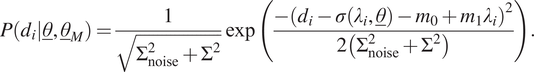 $$ P\left({d}_i|\underline{\theta},{\underline{\theta}}_M\right)=\frac{1}{\sqrt{\Sigma_{\mathrm{noise}}^2+{\Sigma}^2}}\exp \left(\frac{-{\left({d}_i-\sigma \left({\lambda}_i,\underline{\theta}\right)-{m}_0+{m}_1{\lambda}_i\right)}^2}{2\left({\Sigma}_{\mathrm{noise}}^2+{\Sigma}^2\right)}\right). $$
Clearly, $ {\underline{\theta}}_M={\left[{m}_0,{m}_1,\Sigma \right]}^T $
.
$ {\underline{\theta}}_M={\left[{m}_0,{m}_1,\Sigma \right]}^T $
.
4.3. Normal distribution with a quadratic mean
In the next case, the same model uncertainty is again considered, yet the expression of the mean is again changed: a quadratic expression is used, resulting in the following likelihood function for a single measurement:
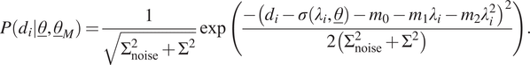 $$ P\left({d}_i|\underline{\theta},{\underline{\theta}}_M\right)=\frac{1}{\sqrt{\Sigma_{\mathrm{noise}}^2+{\Sigma}^2}}\exp \left(\frac{-{\left({d}_i-\sigma \left({\lambda}_i,\underline{\theta}\right)-{m}_0-{m}_1{\lambda}_i-{m}_2{\lambda}_i^2\right)}^2}{2\left({\Sigma}_{\mathrm{noise}}^2+{\Sigma}^2\right)}\right). $$
Therefore, $ {\underline{\theta}}_M={\left[{m}_0,{m}_1,{m}_2,\Sigma \right]}^T $
.
$ {\underline{\theta}}_M={\left[{m}_0,{m}_1,{m}_2,\Sigma \right]}^T $
.
4.4. Mooney–Rivlin hyperelasticity
In the fourth case, model uncertainty is chosen in the same way as before, except that the mean behaves according to the second term of standard Mooney–Rivlin hyperelasticity. As the stress–stretch relation for standard Mooney–Rivlin hyperelasticity in a tensile/compression experiment is expressed according to Equation (9), the likelihood function for a single measurement is now expressed as follows:
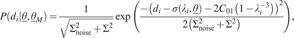 $$ P\left({d}_i|\underline{\theta},{\underline{\theta}}_M\right)=\frac{1}{\sqrt{\Sigma_{\mathrm{noise}}^2+{\Sigma}^2}}\exp \left(\frac{-{\left({d}_i-\sigma \left({\lambda}_i,\underline{\theta}\right)-2{C}_{01}\left(1-{\lambda}_i^{-3}\right)\right)}^2}{2\left({\Sigma}_{\mathrm{noise}}^2+{\Sigma}^2\right)}\right), $$
where we repeat for clarity that the expression for $ \sigma \left({\lambda}_i,\underline{\theta}\right) $
is given in Equation (7). In this case,
$ \sigma \left({\lambda}_i,\underline{\theta}\right) $
is given in Equation (7). In this case, $ {\underline{\theta}}_M={\left[{C}_{01},\Sigma \right]}^T $
.
$ {\underline{\theta}}_M={\left[{C}_{01},\Sigma \right]}^T $
.
4.5. Yeoh model
The fifth case is the same as the previous cases, except that the mean is now taken as the last two terms of Yeoh hyperelasticity. This type of model uncertainty is of course chosen here, because we know that the synthetic data are generated using Yeoh hyperelasticity, but also in a real-world scenario, it makes sense to use a more advanced model than Neo-Hookean hyperelasticity (or Mooney–Rivlin hyperelasticity for that matter as it gives almost the same response for uniaxial tension as Neo-Hookean hyperelasticity). This yields the following likelihood function for a single measurement:
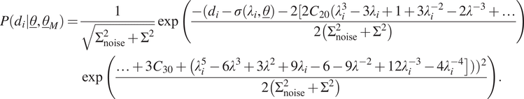 $$ {\displaystyle \begin{array}{l}\hskip0.36em P\left({d}_i|\underline{\theta},{\underline{\theta}}_M\right)=\frac{1}{\sqrt{\Sigma_{\mathrm{noise}}^2+{\Sigma}^2}}\exp \left(\frac{-({d}_i-\sigma \left({\lambda}_i,\underline{\theta}\right)-2[2{C}_{20}({\lambda}_i^3-3{\lambda}_i+1+3{\lambda}_i^{-2}-2{\lambda}^{-3}+\dots }{2\left({\Sigma}_{\mathrm{noise}}^2+{\Sigma}^2\right)}\right)\\ {}\hskip4.8pc \exp \left(\frac{\dots +3{C}_{30}+\left({\lambda}_i^5-6{\lambda}^3+3{\lambda}^2+9{\lambda}_i-6-9{\lambda}^{-2}+12{\lambda}_i^{-3}-4{\lambda}_i^{-4}\right]\left)\right){}^2}{2\left({\Sigma}_{\mathrm{noise}}^2+{\Sigma}^2\right)}\right).\end{array}} $$
In this case, $ {\underline{\theta}}_M=\left[{C}_{20},{C}_{30},\Sigma \right] $
.
$ {\underline{\theta}}_M=\left[{C}_{20},{C}_{30},\Sigma \right] $
.
4.6. Gaussian process
In the last case, we consider model uncertainty in the form of a GP with a zero mean. GP provides a solution to modeling arbitrary function by letting the data choose the complexity of the response. This form of model uncertainty is inherently different from the previous ones, because it involves a correlation between all the inputs. Consequently, the final likelihood function cannot be formulated as a multiplication of different likelihood functions, each associated with a single measurement (i.e., Equation (20) cannot be used). Instead, the final likelihood function must directly be expressed for all $ {n}_m $
measurements. The final likelihood function reads:
$ {n}_m $
measurements. The final likelihood function reads:
 $$ P\left(d|\underline{\theta},{\underline{\theta}}_M\right)=\frac{1}{\mid \underline {\underline{\Sigma}}+{\Sigma}_{\mathrm{noise}}\underline {\underline{I}}\mid}\exp \left(-\frac{1}{2}{\left(\underline{d}-\underline{\sigma}\left(\lambda, \underline{\theta}\right)\right)}^T{\left(\underline {\underline{\Sigma}}+{\Sigma}_{\mathrm{noise}}\underline {\underline{I}}\right)}^{-1}\left(\underline{d}-\underline{\sigma}\right(\lambda, \underline{\theta}\left)\right)\right), $$
where $ \mid \bullet \mid $
denotes the determinant of a matrix,
$ \mid \bullet \mid $
denotes the determinant of a matrix, $ \underline {\underline{I}} $
an
$ \underline {\underline{I}} $
an $ {n}_m\times {n}_m $
diagonal identity matrix, and
$ {n}_m\times {n}_m $
diagonal identity matrix, and $ \underline {\underline{\Sigma}} $
the
$ \underline {\underline{\Sigma}} $
the $ {n}_m\times {n}_m $
(symmetric) covariance matrix associated with the GP, of which the component at row
$ {n}_m\times {n}_m $
(symmetric) covariance matrix associated with the GP, of which the component at row $ i $
, column
$ i $
, column $ j $
is formulated as follows:
$ j $
is formulated as follows:
 $$ {\left(\underline {\underline{\Sigma}}\right)}_{ij}={c}^2\exp \left(\frac{-{\left({\lambda}_i-{\lambda}_j\right)}^2}{2{\psi}^2}\right). $$
Two model uncertainty parameters are, therefore, associated with the GP: $ {\underline{\theta}}_M={\left[c,\psi \right]}^T $
.
$ {\underline{\theta}}_M={\left[c,\psi \right]}^T $
.
5. Results
In this section, the results for the different forms of model uncertainty are compared to each other. The measurement data are artificially generated (it is supposed that experimental data are not correlated) with the Yeoh model with $ {C}_{10}=1.2\mathrm{MPA} $
,
$ {C}_{10}=1.2\mathrm{MPA} $
, $ {C}_{20}=-0.057\mathrm{MPA} $
, and
$ {C}_{20}=-0.057\mathrm{MPA} $
, and $ {C}_{30}=0.004\mathrm{MPA} $
. The measurement noise is generated using a normal distribution with a zero-mean variance of
$ {C}_{30}=0.004\mathrm{MPA} $
. The measurement noise is generated using a normal distribution with a zero-mean variance of $ {\Sigma}_{\mathrm{noise}}=0.5\mathrm{MPA} $
. The model of interest is Neo-Hookean hyperelasticity, entailing that we are interested in parameter
$ {\Sigma}_{\mathrm{noise}}=0.5\mathrm{MPA} $
. The model of interest is Neo-Hookean hyperelasticity, entailing that we are interested in parameter $ {C}_{10} $
.
$ {C}_{10} $
.
In the diagrams that follow below, both the posterior predictive (PP) check and the highest-posterior density (HPD; also known as the credible interval) are presented. The PP check generates “new observations,” although they are presented as bands in the diagrams below. The new observations can be used to interpolate or extrapolate the model or to investigate whether or not the model is able to emulate the (old) measurements that were used to identify its parameters and uncertainties. The former is performed (i.e., assessing if the old measurements are within the same band as the new measurements).
In order to generate the new observations, the PP check uses the posterior distribution and the noise distribution (i.e., the likelihood function) as follows:
 $$ P\left(\hat{d}|\underline{d}\right)=\int \int P\left(\hat{d}|\underline{\theta},{\underline{\theta}}_M\right)P\left(\underline{\theta},{\underline{\theta}}_M|\underline{d}\right)d\underline{\theta}d{\underline{\theta}}_M, $$
where $ \hat{d} $
denotes a new measurement.
$ \hat{d} $
denotes a new measurement.
To work out the integral in Equation (27), one can first take a sample for $ \underline{\theta} $
and
$ \underline{\theta} $
and $ {\underline{\theta}}_M $
from posterior distribution
$ {\underline{\theta}}_M $
from posterior distribution $ P\left(\underline{\theta}|\underline{d}\right) $
, and then use this sample in the likelihood function to obtain the new measurement,
$ P\left(\underline{\theta}|\underline{d}\right) $
, and then use this sample in the likelihood function to obtain the new measurement, $ \hat{d} $
.
$ \hat{d} $
.
The HPD interval is a commonly used method to explain the spread of the posterior distribution. The smallest interval containing an $ X $
percent of the probability density is called the
$ X $
percent of the probability density is called the $ X\% $
HPD. In the present contribution, the
$ X\% $
HPD. In the present contribution, the $ 95\% $
HPD is used to compare the influence of the different forms of model uncertainty.
$ 95\% $
HPD is used to compare the influence of the different forms of model uncertainty.
It should be noted that in all parts of this study, an uninformative prior distribution (i.e., a uniform distribution) with a wide interval is used, which implies that the posterior is effectively governed by the inference of the experimental data.
It is also worth to note that in order to obtain the results of this section, all posteriors are numerically sampled. Instead of a random walk sampler, such as the Metropolis–Hastings algorithm, an HMC sampler is used. Where random walk samplers only require posterior evaluations, HMC samplers also require the gradient of the posterior. Thanks to the gradient information, HMC samplers need less samples to evaluate posteriors than random walk samplers, entailing that HMC samplers are an order of magnitude faster than random walk samplers (Beskos et al., Reference Beskos, Pillai, Roberts, Sanz-Serna and Stuart2013; Betancourt, Reference Betancourt2017).
5.1. Polynomial model uncertainty
Figure 1a presents the PP check for Neo-Hookean hyperelasticity without any model uncertainty. It is clear that the previous measurements are not contained in the bands formed by the new measurements. This stems from the fact that the synthetic data are generated from Yeoh hyperelasticity. Figure 1b, c makes clear that incorporating model uncertainty as a normal distribution with a constant mean or a linear input-dependent mean hardly changes the results. For the linear input-dependent mean, this can be explained by the fact that the Neo-Hookean response itself also contains a linear dependency. If model uncertainty consists of a normal distribution with a quadratic input-dependent mean, the results are substantially better (Figure 1d). This can be explained by the fact that the quadratic dependency of the model uncertainty is not present in the Neo-Hookean response.
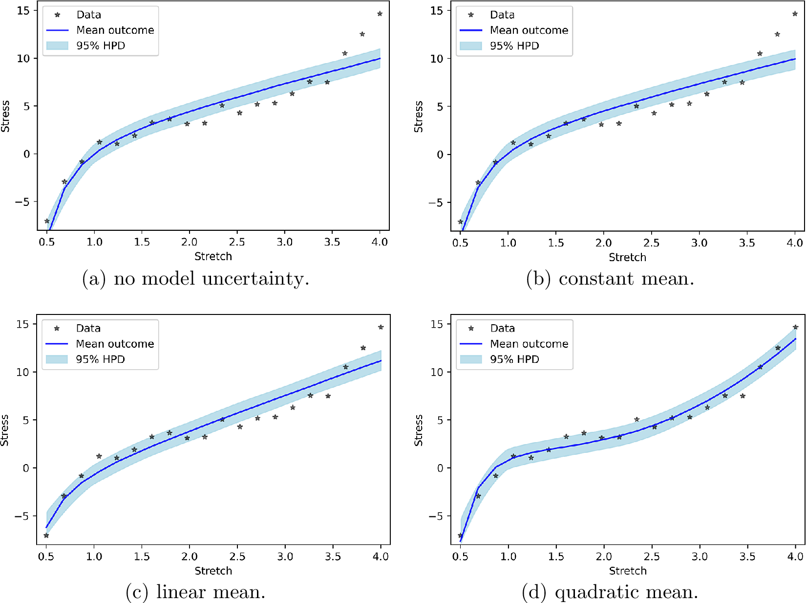
Figure 1. posterior predictive check for polynomial model uncertainty.
We believe that it is interesting to reveal how much of the “work” to generate the new measurements (according to the PP check) is performed by the model and how much by the model uncertainty. To this end, Figure 2 presents the PP check by considering that only the model is used to generate the new observations. In other words, even though the probabilistic identification is performed using model uncertainty, Equation (27) is replaced by:
 $$ P\left(\underline {\hat{d}},\underline{d}\right)=\int P\left(\underline {\hat{d}}|\underline{\theta}\right)P\left(\underline{\theta}|\underline{d}\right)d\underline{\theta}. $$
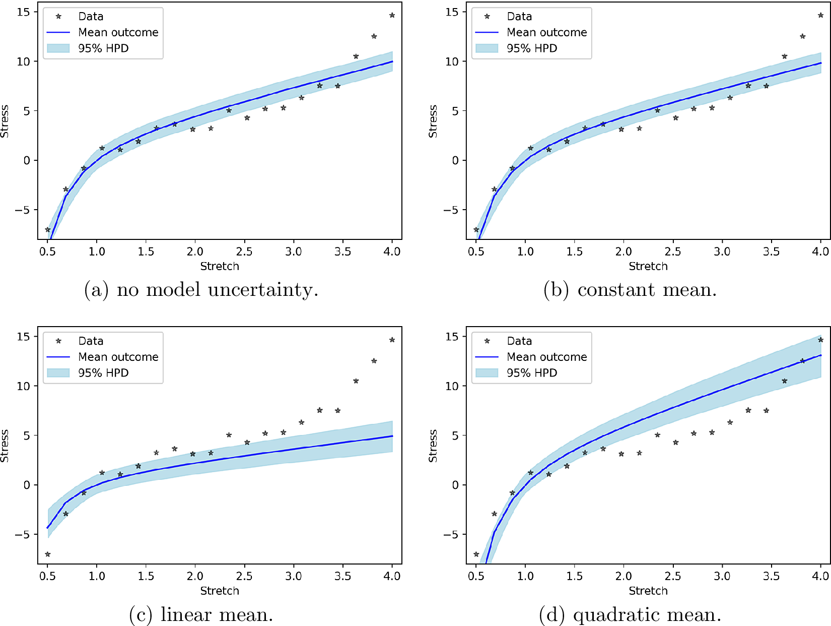
Figure 2. Posterior prediction for polynomial model uncertainty functions without work done by model uncertainty.
It is easy to see that in case of a constant and a linear input-dependent mean, the model uncertainty hardly performs any work. In case of the quadratic input-dependent mean, on the other hand, the model uncertainty can substantially improve the prediction.
5.2. Hyperelastic model uncertainty
In this part, we consider model uncertainty as a normal distribution with an input-dependent mean where the input-dependency follows the response of more complex hyperelastic models than Neo-Hookean hyperelasticity. We consider the mean to behave according to the parts of the Mooney–Rivlin response and the Yeoh response that are not present in the Neo-Hookean response. Figure 3b shows that the PP checks of Mooney–Rivlin model uncertainty and without model uncertainty are practically the same. This can be explained by the fact that the uniaxial tensile/compression responses of Neo-Hookean and Mooney–Rivlin hyperelasticity are similar. Consequently, a mean according to the part of the Mooney–Rivlin response that is not present in the Neo-Hookean response hardly improves the prediction. As the part of the Yeoh response for uniaxial loading that is not present in the Neo-Hookean response is substantially different from the Neo-Hookean response, Yeoh model uncertainty relatively accurately describes the mismatch between model and measured data (Figure 3c).
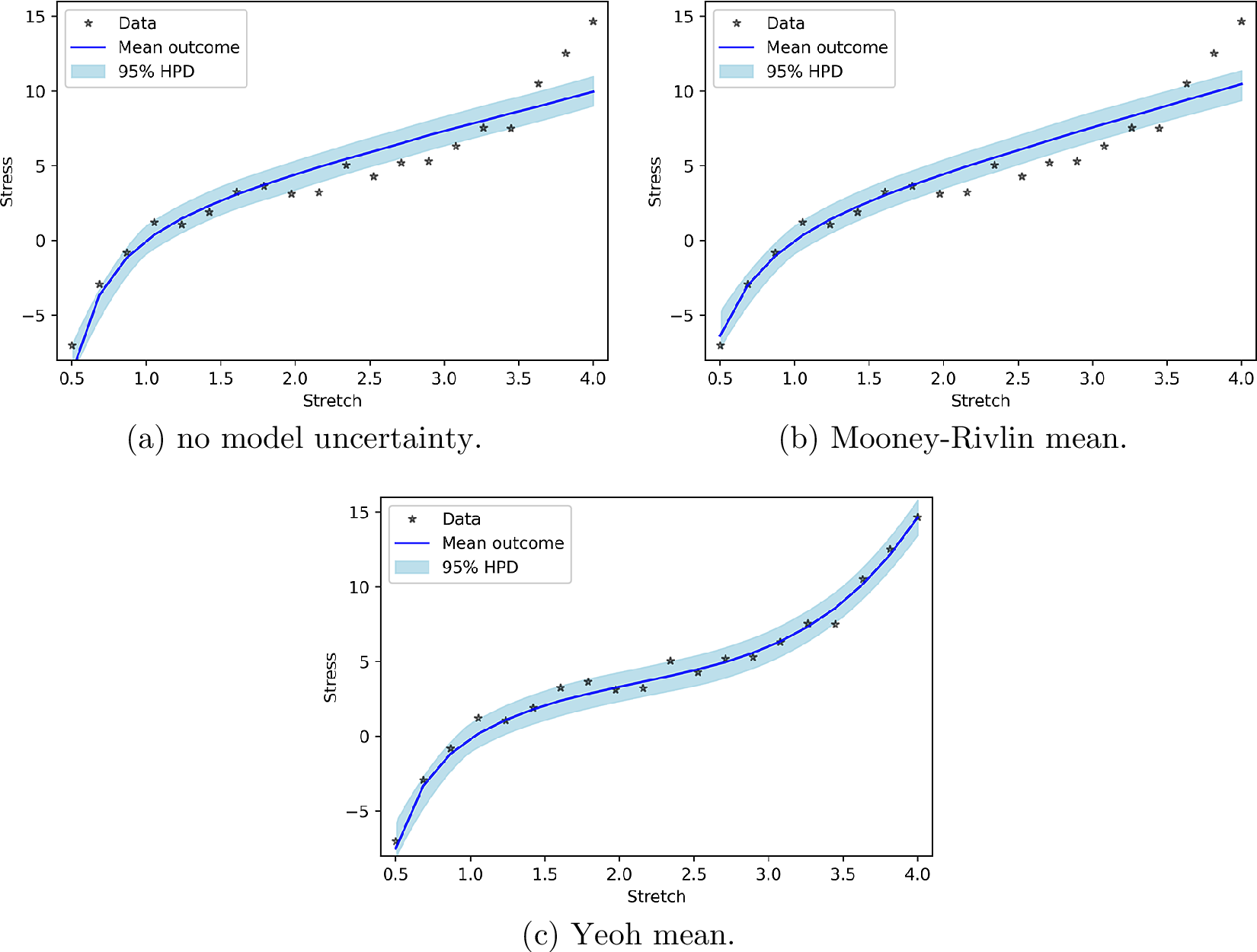
Figure 3. Posterior prediction for hyperelastic model uncertainty functions.
In order to again reveal to which amount the new measurements of the PP check are due to the work of the model and the model uncertainty, we present the PP check for the model alone (i.e., according to Equation (28)). Figure 4 presents these results. Figure 4 shows that the improvement in Figure 3c is due to the effect of model uncertainty terms and not the model itself.
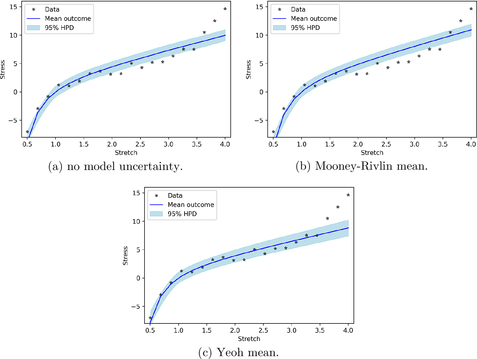
Figure 4. Posterior prediction for hyperelastic model uncertainty functions without work done by model uncertainty.
5.3. Gaussian process as model uncertainty
As the last case, model uncertainty is considered as a GP. In this model, no a priori shape (linear, quadratic, or etc.) imposed on the model uncertainty, and we let the GP to decide its shape. Figure 5 shows the PP for the GP model uncertainty. One can see that the results are completely in line with the measured data. In addition, similar to previous cases, Figure 6 indicates that the performance of Neo-Hookean hyperelasticity itself without considering the GP parameters are poor.
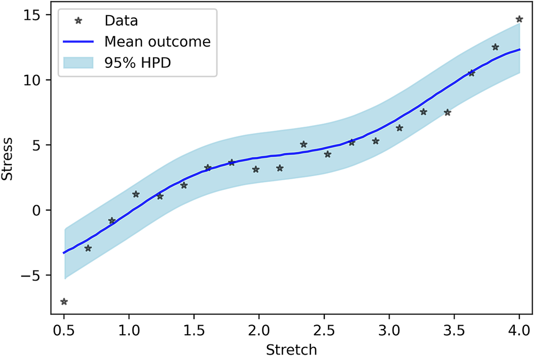
Figure 5. Posterior prediction for considering Gaussian process as model uncertainty.
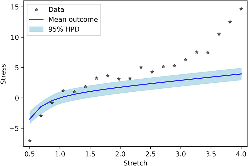
Figure 6. Posterior prediction for Gaussian process without work done by model uncertainty.
5.4. Marginal posteriors
Model uncertainty is often used to achieve a better fit between the PP check and the old measurements, assuming one is solely interested in the responses of Figures 1, 3, and 5. In computational (bio)mechanics, the aim is to use model uncertainty to make predictions for other models than the ones used to identify the parameter uncertainties (e.g., to use the identified parameter uncertainty for finite element simulations). In other words, we aim to employ model uncertainty not to make the PP check better fit the old measurements, but to ensure that the uncertainty of $ {C}_{10} $
is better identified.
$ {C}_{10} $
is better identified.
From this perspective, the aforementioned PP checks (Figures 1, 3, and 5) are not the main interest (which is why we have also shown PP checks without the influence of model uncertainty in Figures 2, 4, and 6), but the marginal posteriors with respect to $ {C}_{10} $
. Figure 7 depicts the marginal posteriors with respect to
$ {C}_{10} $
. Figure 7 depicts the marginal posteriors with respect to $ {C}_{10} $
for different types of model uncertainty. It is clearly visible that the marginal posterior for the Yeoh model as model uncertainty incorporates the true value close to true value. Constant mean model uncertainty estimates
$ {C}_{10} $
for different types of model uncertainty. It is clearly visible that the marginal posterior for the Yeoh model as model uncertainty incorporates the true value close to true value. Constant mean model uncertainty estimates $ {C}_{10} $
similar to the based model prediction. Another interesting point is that although quadratic mean was successfully passed the PP check, it cannot predict
$ {C}_{10} $
similar to the based model prediction. Another interesting point is that although quadratic mean was successfully passed the PP check, it cannot predict $ {C}_{10} $
.
$ {C}_{10} $
.
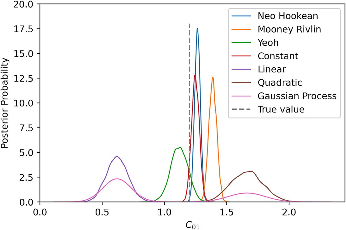
Figure 7. Marginal posteriors for $ {C}_{10} $
.
$ {C}_{10} $
.
6. Conclusion
In this work, a Bayesian paradigm is employed to identify the parameter uncertainties of Neo-Hookean incompressible hyperelasticity based on tensile/compression data. (Synthetic data were generated in order to enable a quantitative comparison.) The aim of the work was to investigate the influence of different forms of model uncertainties. To this end, we have studied six types of model uncertainties:
-
1. A random variable associated with a normal distribution with a constant mean and variance;
-
2. A random variable associated with a normal distribution with a linear input-dependent (stretch-dependent) mean;
-
3. A random variable associated with a normal distribution with a quadratic input-dependent mean;
-
4. A random variable associated with the second term of Mooney–Rivlin hyperelasticity;
-
5. A random variable associated with the last two terms of Yeoh hyperelasticity;
-
6. A GP with a stationary covariance function.
Two lessons can be learned from this study. First, the fact that old measurements fall well within the bandwidth of the posterior predictions does not mean that the parameter uncertainties encompass the true parameter value(s). This was the case for model uncertainty modeled as a GP and for model uncertainty modeled as a random variable coming from a normal distribution with a quadratic input-dependent mean.
Second, incorporating model uncertainty does not guarantee that the parameter uncertainties encompass the true parameter value(s) better. We have observed that of the six types of model uncertainties, only two (model uncertainty as Yeoh hyperelasticity and model uncertainty as a random variable coming from a normal distribution with a constant mean) encompass the true value better than ignoring model uncertainty altogether.
The fact that, in most of the cases, model uncertainty yielded worse results shows, on the one hand, that it should only be used in a careful manner. For incompressible hyperelasticity, it seems that a more sophisticated hyperelastic model than is to be identified can be a good form of model uncertainty. More generally speaking, however, the results indicate the need for a framework that is able to decide by itself to what extent model uncertainty must be applied.
Funding Statement
The project is funded by European Union’s Horizon 2020 research and innovation program under the Marie Sklodowska-Curie grant agreement No.764644.
Competing Interests
The authors declare no competing interests exist.
Data Availability Statement
Data have generated artificially as stated in the paper. Rest of the visualization codes and data are available on reasonable request from the corresponding author.
Author Contributions
Conceptualization, S.P.A.B. and L.A.A.B.; Methodology, M.Z.; Formal analysis, L.A.A.B.; Writing-original draft, M.Z.; Writing-review & editing, M.Z. and L.A.A.B.; Supervision, S.P.A.B. and L.A.A.B.; Funding acquisition, S.P.A.B. All authors approved the final submitted draft.


 Open access
Comments
No Comments have been published for this article.