
Although it has been 30 years after the first studies on muscle and nerve ultrasound imaging that opened a new era of neuromuscular diagnostics,Reference Heckmatt and Dubowitz 1 , Reference Fornage 2 neuromuscular ultrasound still seems to be an unknown option for many clinicians working in the neurological field. Whereas neuroimaging rapidly became the first-line diagnostic modality for patients with central nervous system pathology after the advent of CT scanning in the 1970s, most clinicians investigating peripheral nervous system (PNS) diseases still rely on blood tests, electrophysiology (nerve conduction study and electromyography [EMG]) and muscle or nerve biopsies to confirm their diagnostic suspicions. Even though laboratory testing, EMG and biopsies are proven techniques for many neuromuscular disorders, there is no reason why the PNS could, or should, not be imaged. Quite the contrary, imaging techniques, including CT, MRI and ultrasound, have shown that they can provide valuable additions to an efficient and effective diagnostic workup for suspected neuromuscular disease.Reference Stoll, Wilder-Smith and Bendszus 3 - Reference Masdeu and Gilberto Gonzalez 5
Neuromuscular ultrasound is a rapidly evolving technique for diagnosing, monitoring and facilitating treatment of patients with muscle and nerve disorders.Reference Walker 6 , Reference Walker and Cartwright 7 Ultrasound has some generic advantages over other imaging modalities in that it is a portable, bedside point-of-care technology that is non-invasive, painless and does not involve ionizing radiation. It can visualize muscle texture changes indicating dystrophic changes or denervation, and it has dynamic imaging capabilities that can also capture contractions and fasciculations. The current equipment has excellent tissue resolution in the superficial tissue layers that will show nerve fascicles and continuity even of smaller skin branches. Ultrasound can also provide real-time guidance for needle placement during EMG, lumbar puncture, tissue biopsies and injections such as botulinum toxin or treatment of meralgia paresthetica.Reference Boon, Oney-Marlow, Murthy, Harper, McNamara and Smith 8 - Reference Strakowski 10 It can sometimes make a diagnosis when EMG is not tolerated or non-informative—for example, by helping to localize pathology when all responses are absent.Reference Arumugam, Razali, Vethakkan, Rozalli and Shahrizaila 11 , Reference Smith, Miller and Carroll 12
This review will focus on the technical and practical aspects of ultrasound as an imaging technique for muscles and nerves. It can be used as a “how-to” guide to get started with neuromuscular ultrasound in daily practice, to implement a diagnostic tool that adult and pediatric neurologists, clinical neurophysiologists and other specialists can use for patient-friendly, point-of-care imaging.
Principles of Neuromuscular Ultrasound
Introduction of Ultrasound as an Imaging Technique
Ultrasound imaging is based on reflections that are created when the ultrasound beam encounters a transition between tissues with different sound velocities and gets reflected back to the transducer. Normal human muscle tissue has relatively few such transitions, which provides a relatively black appearance on the screen. In transverse images, this has been dubbed a “starry night” appearance: a black night sky (the muscle fiber tissue) with speckles that look like stars (the fascia structures; Figure 1A). Longitudinally, the muscle fascicle architecture become visible, which shows as a linear (Figure 1B), bi-pennate or triangular structure in the ultrasound image. Normal peripheral nerves look like round, oval, flat or triangular structures with a white edge (the epineurial rim), filled with black dots of varying sizes (the nerve fascicles; Figure 2A). In a longitudinal view they look like a set of railroad tracks (Figure 2B).
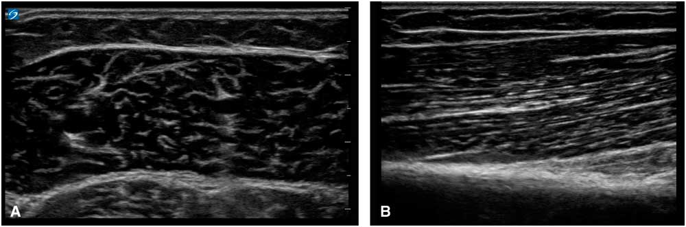
Figure 1 (A) Shows a transverse image of a healthy medial gastrocnemius muscle, showing the “starry night” appearance of dark muscle fiber tissue interspersed with white speckles of fascia. (B) Shows a longitudinal image of a healthy biceps brachii muscle, showing the linear arrangement of muscle fibers that insert at an angle onto the underlying fascia and bone.
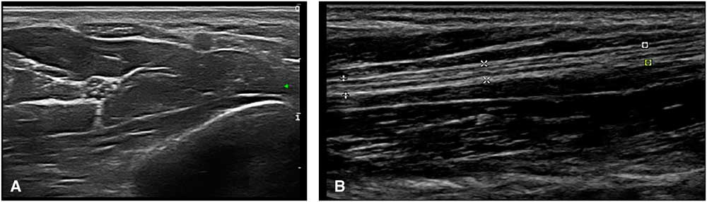
Figure 2 (A) Shows a transverse image of the median nerve in the forearm. The hyperechoic rim of the epineurium and the internal fascicle bundles are clearly visible. (B) Shows a longitudinal image of the median nerve in the forearm. The markers delineate the outer epineurial edge of the nerve; internally, the longitudinal lines of perineurial fascia are seen. The nerve as a whole resembles a set of railway tracks.
Ultrasound Transducers
Ultrasound waves are generated by transducers. The transducers contain piezo-electric elements that convert electricity into sound waves, send an ultrasound beam into the tissue of interest and then transform the reflected ultrasound waves (“backscatter”) back into electronic information. The amount of ultrasound that gets reflected back to the transducer (i.e., the loudness in decibels) determines how black, gray or white the image will look on the screen. No sound (0) results in black pixels and maximum loudness (255) in white pixels, with all levels of gray (1-254) in between. The time it takes for the ultrasound to travel from the transducer to the tissue of interest and back to the transducer is interpreted by the machine to represent the depth of the tissue reflection. The frequency of the ultrasound waves that are sent into the body determines the basic lateral and depth resolution of the image. Low frequencies (e.g., 1-5 MHz) can penetrate deep into the body but have poor lateral resolution; high frequencies (e.g., 15-20 MHz) penetrate only a few centimeters but show excellent lateral resolution. Current ultrasound techniques can display tissue with resolutions up to 0.1 mm,Reference Cosgrove, Meire and Lim 13 which is higher than the resolution that can be achieved with 3 Tesla MRI that has a resolution of up to 0.2×0.2×1.0 mm.Reference Saupe, Prüssmann, Luechinger, Bösiger, Marincek and Weishaupt 14 To achieve optimal images, neuromuscular ultrasound uses transducers with a linear footprint (i.e., the rubber surface that is held against the skin) that can generate ultrasound frequencies of about 5-20 MHz. Although frequencies of around 10 MHz are usually sufficient and practical for muscle imaging, nerve ultrasound requires frequencies around 15 MHz to achieve resolution up to the fascicle level that will also enable the scanning of small sensory skin nerves. For scanning very deep nerves, for example, the sciatic in the gluteal region, or for ultrasound guidance of a lumbar puncture, a low-frequency (around 5 MHz) convex footprint probe such as that used for abdominal exams is advisable.
Ultrasound Image Formation
Many factors influence how a muscle or nerve will look on the screen. Every ultrasound machine has a specific set of image-forming properties that determine how the software handles the incoming sound waves from the transducer elements. These system settings, such as the overall gain (i.e., the volume knob), image depth, focal zones, image compression, the use of harmonic waves and spatial or time-averaging techniques create a specific “look” (Figure 3), and most users will become familiar over time with their standard preset images of muscle or nerve. If image clarity and resolution are paramount, as in nerve ultrasound, one wants a machine that can utilize all image optimization tools to provide the best picture. However, if obtaining reproducible and quantifiable images of muscle echogenicity is the goal, a machine with precisely defined preset and no image-enhancing features is ideal (Figure 4).
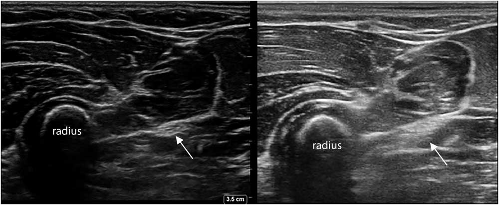
Figure 3 Two transverses images of the proximal ventroradial forearm, showing the bony structure of the radius with different muscles layered on top, and the median nerve between the fascia (arrow). Notice the difference in overall image appearance; the left image was captured with a Sonosite Xporte system with a 5-16 MHz linear probe and a MSK nerve preset (Fujifilm Sonosite Inc., Bothell, Washington, DC), and the right image was captured with an Esaote MyLab Alpha system with a 3-13 MHz linear probe and an MSK preset (Esaote SpA, Genoa, Italy).
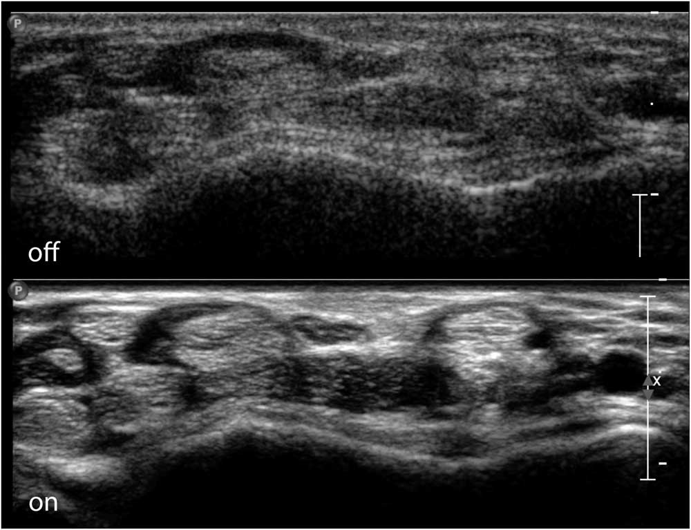
Figure 4 Transverse image of the ventral wrist crease, showing the flexor tendons of the wrist and fingers and the median nerve in the middle on top. The top half of the image shows a raw image format without additional image enhancing; the bottom half shows full use of image-enhancing features with clear delineation of the nerve and tendon contours. Images captured on a Philips IU22 system with a linear 5-17 MHz probe and MSK preset (Philips Healthcare, Eindhoven, The Netherlands).
Transducer Handling During Scanning
Ultrasound scanning requires eye-hand coordination. To have optimal control, the probe should be held as if it were a pen or fork, and not as an ice-pick or hammer. Initially it is usually easier to hold the probe with the dominant hand. However, for some anatomical locations, and also for ultrasound-guided interventions such as botulinum toxin or local anesthetic injections, it is much more practical to scan with the non-dominant hand. Hence, one will benefit from learning to perform ultrasound with both hands. The probe cord is usually heavy and will tilt the probe if not suspended, so wrapping it around the operator’s neck, arm or little finger will allow better control of the probe angle.
To facilitate hand-eye coordination training, it is usually easiest to start scanning transverse images while keeping what is on the left side of the probe to the left side of the image on screen. This will assure that when the probe is moved, the anatomy moves in the same direction, making it easier for the brain to make course corrections and track anatomical structures. This is again especially important for needle guidance, as it is very counter-intuitive if the hand moves the needle in one direction and the image on screen moves the other way. Most ultrasound transducers have a marker to facilitate alignment. However, the most foolproof way of identifying what is left and right on the probe and screen is to put some gel on the probe, tap on, for example, the left side and see whether the left side of the screen image shows the tapping. For longitudinal (or sagittal) images, the convention is to point the left side of the probe and screen cranially and the right side of the image caudally. This is practical in, for example, diaphragm muscle imaging, as the lung can be seen moving into the image from left to right during normal inspiration, but might move from right to left in case of a paradoxical breathing pattern.
It is also important to consider the setup of the ultrasound exam room and equipment. For instance, with the patient, exam table and machine in place, can one still reach for the machine control buttons to freeze or adjust the image quality if needed? Ideally, one should be able to look at the screen, the probe (and maybe the needle) and the patient at the same time for optimal ergonomics and interaction.
How to Obtain Good Ultrasound Images
The most important aspect of transducer handling to create optimal nerve and muscle ultrasound images is choosing and maintaining a correct scan angle. It cannot be emphasized enough how crucially important it is to have a perpendicular scan angle to the tissue of interest to get a good image on screen. This is because only sound waves that are reflected back to the transducer will produce image information for the machine. Any sound waves that get deflected away from the transducer will not add to the image (Figure 5), thus leaving the image black. This means that in practice even a small scan angle difference of 5° from the perpendicular angle (i.e., 90°) already results in a visibly darker and less informative image; for quantitative measurements of echogenicity, this would be flawed. The tricky part here is that the scan angle difference can both be caused by a slight tilt in the transducer position, as held by the operator, and also by a change of direction or course of the underlying anatomical structure of interest, such as the median nerve in the proximal forearm that runs deep and medially between the two halves of the pronator teres muscle. If the transducer angle is not adjusted to match such a course, the nerve will become blacker and less clearly visible, no matter how many image-enhancing features are used. This also means that, for optimal nerve ultrasound, having a knowledge of the position and course of the nerve of interest in its anatomical context is crucial. It may be necessary to approach the nerve (and hence examine the patient) from different sides during scanning of a whole nerve along its course. For example, the fibular nerve is best imaged at the level of the kneefold with the subject prone, and its proximal part below the biceps femoris tendon running toward the fibular head can be visualized if the transducer is rocked a little more laterally. However, once the nerve circles the fibular head, it is far easier to get a good angle on it and follow it all the way to the ankle when the subject is supine. The only nerve segments that are relatively black without much fascicular architecture, regardless of the scan angle, are the extraforaminal cervical roots that form the brachial plexus. This is because the roots have a relatively lower connective tissue content (around 20%), which means they have fewer reflective structures for ultrasound. The more distal nerve segments have a higher connective tissue content (around 40%-55%), making the fascicles, perineurium and epineurium more visible.Reference Schraut, Walton and Bou Monsef 15
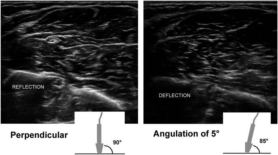
Figure 5 Two images of the proximal ventral forearm showing the flexor muscle overlying the radius (on the left) and ulna (right), with the median nerve in the middle left. The left image shows the result of an optimal 90° scan angle, with clear reflection of the bony edges, the fascia and outline of the nerve. The right image shows a 5° probe tilt with a resulting 85° scan angle toward the bones and fascia; the amount of ultrasound that is deflected and does not return to the probe results in a visibly darker image with suboptimal delineation of anatomical structures.
Anatomy and Landmarks for Imaging
For scanning nerves, it is advisable to start out using a landmark point where the nerve can always be found and identified, independent of the subjects’ build or pathology. For the median nerve, this could be at the level of the wrist crease, where the nerve is very superficial, lying on top of the flexor tendons (Figure 6). The ulnar nerve is easy to pick up in the medial-posterior side of the distal upper arm, and the peroneal (fibular) nerve can always be found in a transverse image of the lateral half of the kneefold. From such a landmark point, the nerve can be tracked both distally and proximally. Backtracking the nerve can also help identify other nerves, such as the tibial and sciatic nerve that come into view when the peroneal (fibular) nerve is followed proximally in the distal upper leg. As a rule, one should always aim to positively identify the nerve that is being scanned, by following it along its known anatomical course to see whether it behaves as expected. For example, if a structure looks like a nerve but blends into muscle tissue more proximally, it is identified as a tendon.
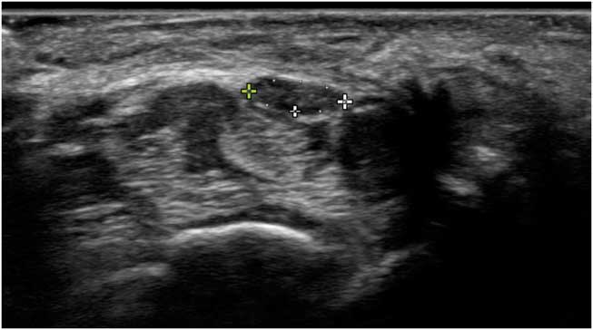
Figure 6 Transverse image of a normal median nerve at the level of the wrist crease, with markers indicating the internal epineurial rim and measuring the cross-sectional area. The nerve lies on top of the finger flexor tendons. The arch of the carpal ligament can be seen lying from left to right over the nerve.
Image Annotation and Measurements
It is advisable to scan the whole nerve along its length, annotate the images, make measurements of nerve size and, if needed, mark the anatomical position. One should annotate each image with, at a minimum, the side measured (e.g., “L” for left), the nerve’s name (e.g., “med” for median) and, for longitudinal images, which side of the image was proximal (e.g., “prox”). If it is unclear from the image at which anatomical site it was taken, annotate that information in the image too (e.g., “distal carpal tunnel;” see Figure 7).
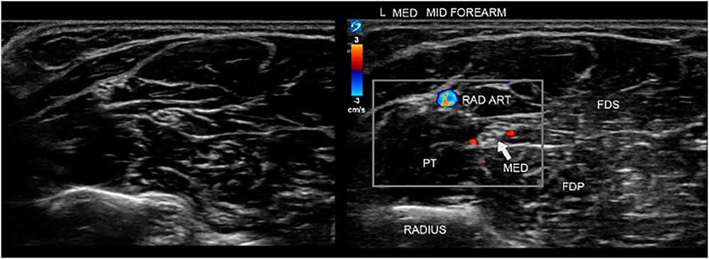
Figure 7 Two images of the ventral forearm. The left image is unannotated, making it harder to instantly recognize the site and anatomical features. On the right is the annotated image indicating the bone, muscles and median nerve for clarity, and also showing power Doppler signals of the radial artery (RAD ART) and small arteries accompanying the median nerve. FDP=flexor digitorum profundus; FDS=flexor digitorum superficialis; PT=pronator teres.
Most nerve pathologies lead to nerve size enlargement because of edema or increased connective tissue formation (scarring). Thus, knowing the normal size of any given nerve at a given anatomical site is paramount for nerve ultrasound assessment. For nerve size measurements, the workhorse is the transverse cross-sectional area (CSA) measurement (Figure 6). Because peripheral nerves can have different shapes, for example, round, oval, oblong or triangular, depending on their anatomic location, transverse CSA is more reliable and reproducible than nerve diameter measurement, and is the most robust measure to confirm nerve pathology.Reference Ažman, Hrabač and Demarin 16 The CSA should be measured within the hyperechoic epineurial rim that encircles the nerve fascicles. This is because the epineurial connective tissue layer surrounding the nerves indistinguishably blends into the connective tissue layers of the surrounding tissues, and hence has no clear outward boundary. Longitudinal images are often visually very informative for the referring physician, but harder to quantify reliably, as how large the diameter will be depends on which slice of the nerve is shown and in which direction the cut is made. Only in perfectly round nerves would the diameter be stable and reproducible from every scan angle.
The transverse CSA of a given nerve shows a distribution within a given population, and the nerve size varies depending on different anthropometric parameters such as age, sex, body size (as reflected by length, weight and body mass index) and racial background. Infants start with nerves that are about half the size (CSA) of an adult nerve; school-aged children are at about 2/3 of adult size. People of different racial backgrounds also show slightly different nerves sizes; for example, people of Asian descent have slightly (around 10%) smaller nerves compared with European Caucasians. The main conclusion to be drawn from these differences is how important it is in practice to use the right reference values for the right patient. If no local values are available, several publications have provided measurements in different populations.Reference Burg, Bathala and Visser 17 - Reference Cartwright, Mayans, Gillson, Griffin and Walker 20
It is also necessary to realize the difference between a population-based reference (such as the mean CSA for a nerve at a given site in healthy adults) and a disease-specific receiver operating curve-based cutoff point (such as the optimal CSA that will tell patients with carpal tunnel syndrome apart from patients with other hand and wrist complaints with the highest sensitivity). These two approaches can lead to very different values, which should not be confused. In practice, it is advisable to use a disease-specific cutoff value of known sensitivity and specificity when available for a specific patient and referral question. However, if no disease-specific cutoff reference exists, a population-based reference value is useful to determine whether the nerve is probably abnormal or not.
Nerve ultrasound scan protocol
Many studies on nerve ultrasound in particular patient groups describe measurement results at predefined anatomical sites, but this is not a very sensible approach from a clinical diagnostic point of view. As, with a little experience, scanning the whole nerve along its length is easily feasible for most limb nerves, it is advisable to examine all nerve segments for pathology. Two studies in suspected carpal tunnel syndromeReference Csillik, Bereczki, Bora and Arányi 21 , Reference Paliwal, Therimadasamy, Chan and Wilder-Smith 22 nicely support this practice by showing that, in addition to scanning the proximal carpal tunnel, scanning the distal carpal tunnel segment will add 15%-20% sensitivity. A practical compromise for a scan protocol is to scan the nerve along its whole length and measure it at a few predefined anatomical sites and at the sites of suspected pathology, and to also make longitudinal images of the latter.
Visual evaluation of nerve appearance
In addition to quantifying nerve size, it is also informative to visually evaluate the appearance of the nerve and its fascicles.Reference Grimm, Winter, Rattay and Härtig 23 Nerves that have suffered mechanical compression or stretch, such as in entrapment or traumatic (or iatrogenic) traction injury, usually become swollen and hypoechogenic, and thus the CSA increases and the fascicles look more black at or just proximal to the site of pathology. With repeated mechanical friction, such as in long-standing carpal tunnel syndrome or ulnar neuropathy at the elbow, the nerve may form a very thick outer epineurial rim, giving the appearance of a thick white band surrounding the fascicles. Actively inflamed nerves—for example, in chronic inflammatory demyelinating polyneuropathy—can become grossly swollen and show fascicles with a diffusely grayish “ground glass” appearance, and a transected nerve will show two swollen stumps a few centimeters apart in a longitudinal image, with no recognizable nerve tissue in between. It is important to look for these associated changes in nerve appearance and capture them transversally and longitudinally for reporting (see Figure 8, e.g., of nerve pathology).
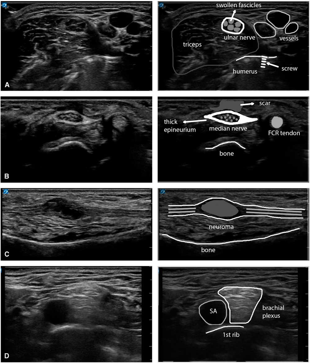
Figure 8 Panel showing four examples of the visual appearance of nerve pathology. (A) Swollen ulnar nerve in the upper arm with enlarged, hypoechoic fascicles and a slightly thicker epineurium, caused by thermal injury of the nerve during surgery for a humeral fracture (osteosynthesis material is visible in the underlying bony structure). (B) Enlarged median nerve at the wrist with a very thick epineurium and an overlying subcutaneous scar, caused by repeated carpal tunnel decompressions in the context of ongoing labor-induced compression of the nerve. (C) Neuroma in continuity of the ulnar nerve in the forearm after a glass-cut injury that partially transected the nerve and encased it in scar tissue (a Sunderland mixed-grade 4/5 lesion). (D) Supraclavicular brachial plexus lying on top of the 1st rib and adjacent to the subclavian artery in a patient with active chronic inflammatory demyelinating polyneuropathy. The different plexus elements are swollen and show a typical diffusely hyperechogenic appearance. FCR=flexor carpi radialis; SA=subclavian artery.
Evaluation of muscle ultrasound
For identification of a specific muscle in its anatomical context and assessing echogenicity, transverse images work best, whereas assessment of fiber direction and disruption (as in muscle tears) and pennation angles require longitudinal images (Figure 1B). Just as with identifying nerves, here too it is advisable to use standard landmarks that will always show the way to the specific muscle of interest. For example, in the ventral upper leg the oval appearance of the rectus femoris with its characteristic internal J-shaped fascia (Figure 9A) is usually easily identified. From this landmark muscle, one can slide the probe laterally to identify the vastus lateralis and, subsequently, when sliding more posteriorly, the biceps femoris, semitendinosus and semimembranosus. For quantitative muscle ultrasound screening, a standardized scanning protocol should be used.
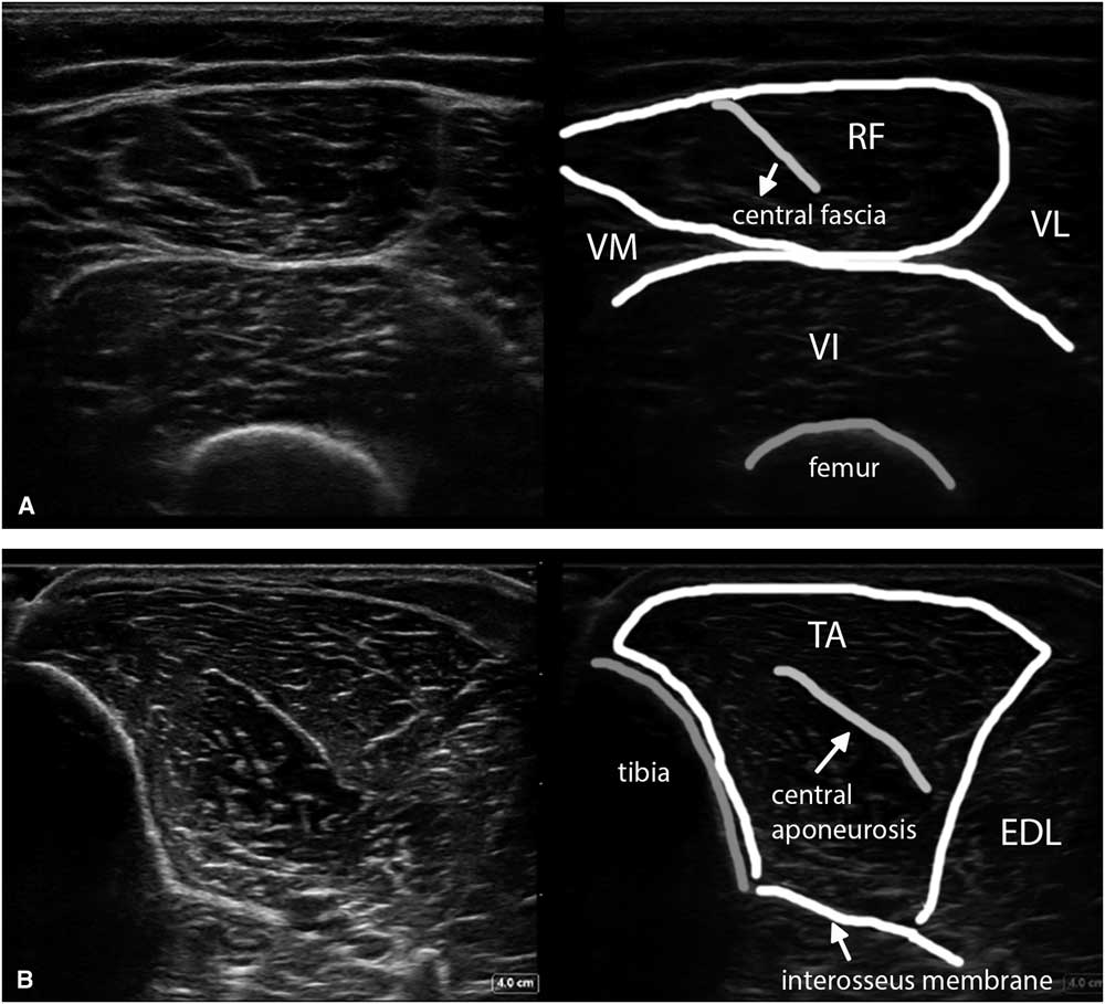
Figure 9 (A) Shows a transverse image of the ventral upper leg (VL), with the rectus femoris (RF) muscle lying in the middle on top, showing the typical oblique shape of its internal central fascia. (B) Shows a transverse image of the tibialis anterior (TA) muscle scanned at a 90° angle to obtain the brightest and best reproducible depiction of the underlying interosseus membrane and equal echogenicity of both muscle halves. EDL=extensor digitorum longus; VI=vastus intermedius; VM=vastus medialis.
To obtain the best reproducibility, the images should be made perpendicular to a reproducible structure such as bone or fascia underlying the muscle—for example, with the femur in the upper leg or the interosseus membrane in the lower leg (Figure 9B). This will ensure maximum reflection of ultrasound and hence the brightest image features on the screen.
Visual evaluation of muscle ultrasound
Visual evaluation is the standard radiologic approach in which the observer just looks at the image and compares it with his or her previous experience with this type of image to conclude whether it is normal or not. Three basic patterns of abnormality are discerned in transverse muscle images (Figure 10): (a) diffuse hyperechogenicity (indicating dystrophy or complete denervation); (b) a moth-eaten pattern with areas of increased echogenicity alternating with normal (i.e., black) appearing “holes” (indicating denervation with partial reinnervation); and (c) normal tissue with focal areas of hyperechogenicity (indicating focal pathology such as inflammation). In all three patterns, the areas of increased echogenicity will absorb and scatter the ultrasound beam, which leads to attenuation and a loss of visibility of the underlying tissue layers on ultrasound (Figure 11). Ultrasound using visual evaluation can be very helpful to screen for neuromuscular pathology in muscles that are difficult to test clinically or with EMG, either because of lack of patient cooperation or a difficult anatomical location (e.g., see Figure 12). In practice, the authors often use it as an adjunct to the electrodiagnostic examination to select the most abnormal muscles for study and to avoid unnecessary needle sticks in muscles that have a normal appearance.
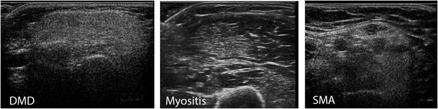
Figure 10 This panel shows three types of abnormality that can be found on visual evaluation of muscle ultrasound. On the left a diffusely increased echogenicity with a “ground glass” aspect of the biceps brachii muscle is seen. This pattern occurs in muscular dystrophies such as Duchenne muscular dystrophy (DMD) and facioscapulohumeral dystrophy (FSHD). In the middle a biceps muscle is seen with an area of increased echogenicity and other parts of the muscle that have a normal appearance. Such patchy abnormalities are mainly found in inflammatory disorders of muscle, such as dermatomyositis, but can also occasionally occur in FSHD or in disorders with very focal denervation such as neuralgic amyotrophy. On the right a biceps muscle with focal zones of normal echogenicity (the black holes) surrounded by hyperechogeneous tissue (denervated fibrosed muscle) is seen, giving it a “moth-eaten” appearance. This pattern is found in disorders with denervation and partial reinnervation of muscles, such as in spinal muscular atrophy (SMA), severe radiculopathies or inclusion body myositis.
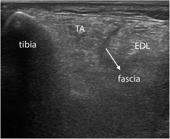
Figure 11 Transverse image of a severely affected tibialis anterior (TA) muscle in facioscapulohumeral dystrophy. The intramuscular central tendon, as well as the intermuscular facia between the TA and extensor digitorum longus (EDL), now appear dark instead of bright (compare to Figure 9B). The interosseus membranes and deeper structures are no longer visible because of attenuation of the ultrasound caused by absorption and scattering of the beam.
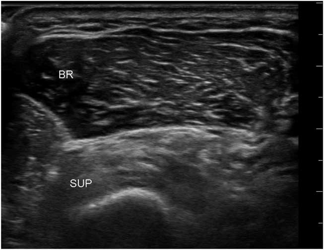
Figure 12 Transverse image of the proximal dorsomedial forearm showing the radius with an overlying supinator and brachialis muscle. The echogenicity of the supinator is clearly abnormal and compatible with selective denervation caused by a partial infraclavicular brachial plexus traction injury. BR=brachioradialis; SUP=supinator.
To improve diagnostic sensitivity, a semi-quantitative score such as the Heckmatt grading scaleReference Heckmatt, Leeman and Dubowitz 24 (Figure 13) can be used to rate the echogenicity of muscle images. Heckmatt grade I corresponds to the appearance of normal muscle, with clearly visible muscle architecture and minimal attenuation of the ultrasound beam, so that underlying structures such as bone and fascial planes are clearly visible. Heckmatt grade 2 denotes a slight overall increase in echogenicity (i.e., whiteness) of the muscle, without attenuation of the underlying structures. Grade 3 shows a further increase in whiteness and some attenuation with reduced visibility of underlying structures; grade 4 shows a completely white muscle and strong attenuation with loss of visualization of the underlying bone or fascia echo.
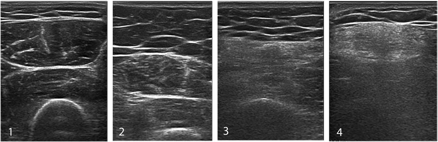
Figure 13 The Heckmatt grading scale for visual assessment of muscle echogenicity. Grade 1 is normal. Grade 2 shows an overall increase in echogenicity without architecture loss or attenuation. Grade 3 showed clearly increased muscle echogenicity, loss of muscle architecture and some attenuation causing less visibility of deeper structures. Grade 4 denotes a completely white muscle with loss of recognizable features and strong attenuation of the ultrasound signal, so no deep structures can be discerned beyond the superficial layer of muscle.
Visual muscle evaluation and grading are both dependent on operator experience. All healthy muscles look slightly different on ultrasound because of differences in architecture and connective tissue content (see e.g., Figures 1, 7A, 11A, 11B). In addition, their echogenicity also strongly depends on age and the fat content of muscle. People aged 40-50 years and over or obese people will have whiter muscles (Figure 14).Reference Arts, Pillen, Schelhaas, Overeem and Zwarts 25 , Reference Nijboer-Oosterveld, van Alfen and Pillen 26 The appearance of normal and diseased muscle will also vary considerably from one ultrasound machine and preset to another, so that using a machine different from the one the examiner is used to will make it much more difficult to assess images correctly (see Figure 5).
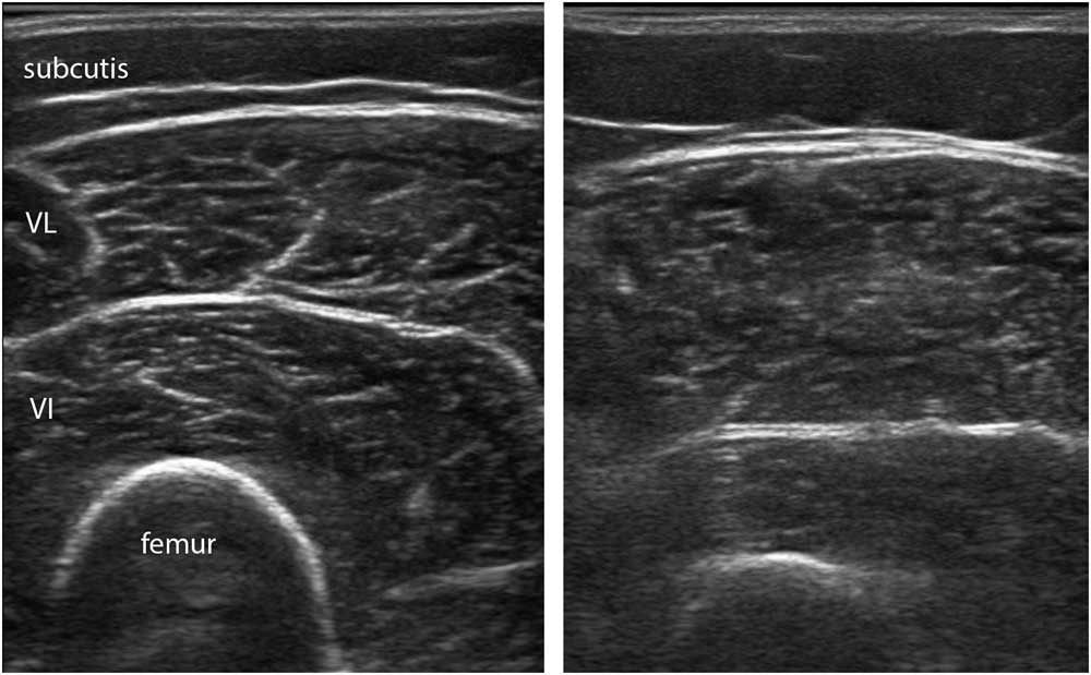
Figure 14 This panel shows the vastus lateralis muscle in two healthy female subjects, one with a body mass index (BMI) of 18.7 (left image) and one with a BMI of 30.1 (right image). The muscle on the right has more intramuscular fat depositions, leading to a more grainy and somewhat fuzzy appearance of the intramuscular fascia.
Quantitative evaluation of muscle ultrasound
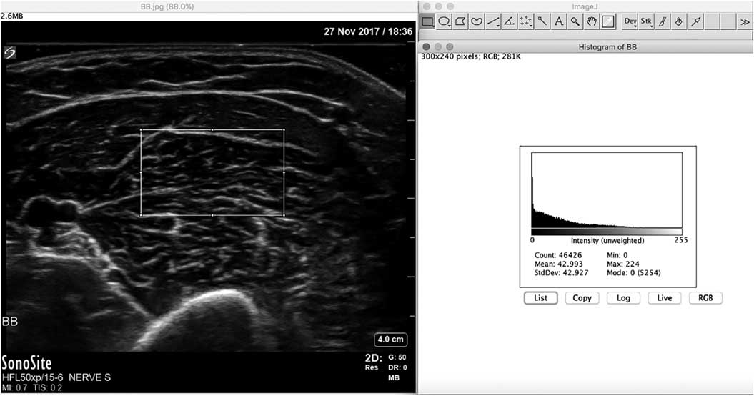
In addition to differences in age, muscle architecture, muscle fat content and system setting, there is yet another reason why visual or semi-quantitative evaluation of muscle has inherent limitations to its sensitivity. The human visual system is designed to be contrast sensitive, which means that when viewing a particular white image the next object viewed will automatically be interpreted to look darker. To overcome all these factors that hamper accurate visual evaluation of muscle images, several quantitative techniques that objectively assess muscle echogenicity have been developed.Reference Mayans, Cartwright and Walker 27 The most robust measures that have also been validated in clinical use are mean grayscale analysis and backscatter analysis.Reference Pillen, Verrips and van Alfen 28 - Reference Shklyar, Geisbush and Mijialovic 31 Grayscale analysis works by selecting a region of interest within the muscle, and having a graphic software program such as ImageJ (freeware, see https://imagej.nih.gov/ij/) to calculate the mean gray value of all the pixels in that region (Figure 15). Usually the mean gray value of 3 separate measurements is averaged to provide a robust value. This mean gray value is then compared with an age-, sex- and weight- or height-matched reference value for that muscle and imaging preset for the specific ultrasound machine and probe used. For this method, a sufficient number of healthy subjects across the sexes and ages will need to be measured to calculate the references for each different muscle. Usually this requires measuring each muscle in at least five males and five females for every decade of age. The measurements in patients are expressed as z-scores, which is the number of standard deviations from the mean echogenicity value for that muscle. To ensure measurement reproducibility between subjects and over time, all system settings that influence the image parameters (both hardware and software) should be maintained constant. Backscatter analysis uses a similarly rigid protocol that compares the measured echogenicity with that of a calibrated phantom.Reference Zaidman, Connolly and Malkus 32
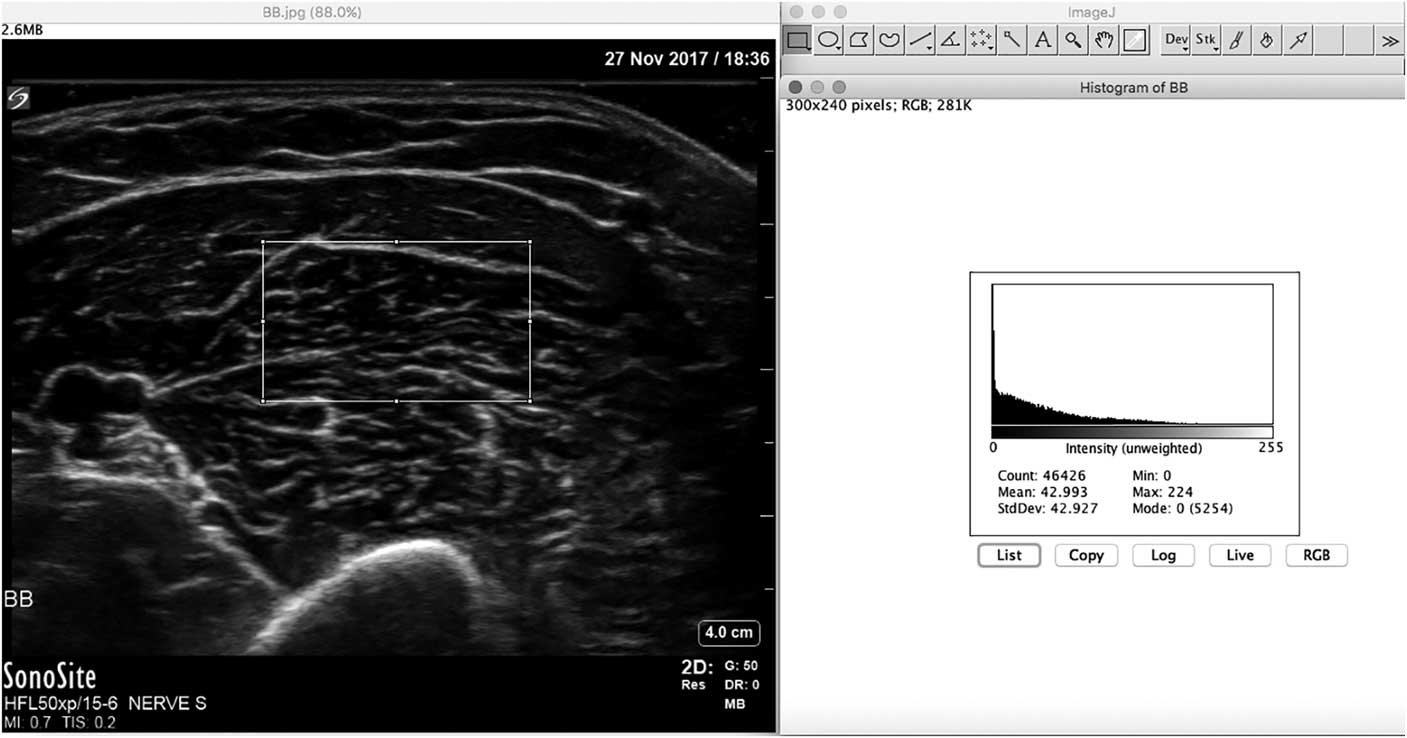
Figure 15 Screenshot of the ImageJ free software program for calculating mean grayscale value from the muscle ultrasound image histogram. The rectangle in the left half of the image denotes the region of interest from which the histogram is captured.
As both techniques require strict protocol adherence across measurements, rigid standardization of software and hardware parameters, and, at least for grayscale analysis, the collection of age-, sex- and weight- or height-matched reference values, the use of quantitative muscle ultrasound is currently limited to centers that routinely scan a large number of patients (e.g., several hundred a year) for clinical or research purposes. In addition, the software- and hardware-dependence of the imaging results precludes sharing reference values across platforms, which currently is an impediment to the distribution of this technique. In spite of these limitations, however, quantitative echogenicity measurements currently have the highest sensitivity and reproducibility for detecting neuromuscular disorders.
Dynamic ultrasound imaging of muscle
A very useful and powerful ultrasound feature is that it allows for dynamic imaging of tissue. Movement of, or within, a muscle can easily be seen and captured using the sequential frame capture (video) feature that is standard on most ultrasound machines. In this way, muscle contractions can be studied, and involuntary movements motor units or muscle fibers such as fasciculations and fibrillations can be visualized. Fasciculations are brisk, randomly occurring contractions of motor units, whose territory is often enlarged by collateral reinnervation in case of a neuromuscular disease. On the ultrasound screen they look like small parts of the muscle, about 0.5-1 cm across, that suddenly and unexpectedly jump (Supplemental Video 1). As ultrasound captures a substantially larger part of the muscle than the EMG needle or visual observation from the outside does, it is not surprising that ultrasound is better at detecting fasciculations than either EMG or clinical observation.Reference Regensburger, Tenner, Möbius and Schramm 33 This makes it very suitable for fasciculation screening, for example, in suspected motor neuron disease. Fasciculations need to be distinguished from contraction pseudotremor (Supplemental Video 2), which is the involuntary firing of one or a few, usually enlarged, neurogenic motor units that shows up on the ultrasound screen as a fixed small area of muscle that twitches almost rhythmically with a predictable pattern of appearance from one twitch to the next. Finally, sometimes under specific circumstancesReference van Alfen, Nienhuis, Zwarts and Pillen 34 even fibrillations can be captured with ultrasound (Supplemental Video 3).
How to Get Started?
Equipment
There are many options on the market for neuromuscular ultrasound imaging. Prices ranged from around $ 25,000 for a basic system with a single transducer to $ 300,000 and over for a full-size radiology system with multiple software options and transducers. Transducers are essential hardware and cost about $ 5000-10,000 each. For a clinician considering buying an ultrasound system, it is important to match the budget and requirements for the system to the different options available. Consider the following questions before making a purchase: Do you want to be able to adjust image formation or just “turn on and scan”? Does the equipment need to be portable, or does the transducer need to be attachable to a smartphone? Does the machine also need to perform vascular scanning, and are extras needed such as needle guidance or three-dimensional imaging ability? It is also advisable to consider other quality conditions such as data storage, network capability and integration with other diagnostic workflow systems.
Some practitioners may only be able to start by sharing a machine with another program or department. In that case one needs to make sure that the machine has the basic imaging properties described above, including a linear transducer in the 5-15 MHz range, with measurement capabilities for diameters and CSAs. From a hospital point of view, time-sharing of an ultrasound machine makes for more efficient use of this expensive equipment. However, in practice, many physicians have found it difficult to match scanning time and schedules, or arrange for joint agreements on servicing and other costs. These “merely practical” issues can all too soon become prohibitive to effective sharing. It makes sense to establish a good rapport with colleagues from another department and assess one another’s specific needs, resources and limits, before setting up such a machine-sharing venture.
Once the equipment is installed, it is advisable to ask the suppliers’ representative to help configure a small number of presets—that is, predefined image acquisition configurations that can usually be selected by pressing a button. Usually a superficial (e.g., 0-4 cm depth range) and a deeper (e.g., 4-8 cm) musculoskeletal ultrasound setting will suffice to get started. To keep it practical, one could try scanning one’s own median nerve and flexor muscles from the wrist to the elbow to see whether the image quality is acceptable with a given preset.
Equipment care and calibrations
As most hospital equipment is written-off over a relatively long period of 7-10 years, it is worthwhile to take good care of the ultrasound equipment to maintain optimal image quality. This goes especially for the transducer footprint, the piezo-electric elements and their wiring. Footprints are usually made of rubber, and this will degrade when cleaned with an alcohol-containing solution. Cleaning the probe and cable after use with inexpensive hydrogen peroxide (H2O2)-based disinfectant wipes will ensure hygienic scanning without degradation of the rubber surface. The transducer cable contains all the wires of the individual piezo-electric elements, very similar to an optic nerve containing nerve fibers from a retina. Avoid bending, kinking, stepping on or driving over the cable, as this will cause individual wires to break, which leads to a progressive dropout of elements, effectively rendering the probe “blind.” It is advisable to have the probe output calibrated regularly—for example, every 1-2 years—to assess remaining power and image quality, and replace the probe if necessary.
Practical issues
To get started, it can be of great help to attend some of the hands-on neuromuscular ultrasound courses that are offered during conferences or in specialized centers. The International Society of Peripheral Neuromuscular Imaging publishes a quarterly digital newsletter that features an overview of training opportunities around the world (e.g., see http://www.ispni-iccnu.org/).
Once the equipment is available and the patients are selected who would benefit from neuromuscular ultrasound, the next challenge is usually to get the machine, the patient and the examiner in the same room at the same time for a long enough period to allow for hands-on trying of the different imaging techniques. It may make sense at first to reserve only the first and last slot of a clinic for ultrasound; starting a little bit earlier with the first patient and ending a bit later with the last will allow oneself to have time to learn. At first, one will need to gain practical experience and confidence in the images made, so it is unwise to try and make reports of findings that will have clinical implications right away. Do scan regularly though and, ideally, review the images and videos with a colleague or an online community forum. After a while one will become confident with the structures that were scanned, and at this point one can start adding the ultrasound information to the patient report or chart, and start scheduling a specific ultrasound clinic. For result reporting, it is recommended to follow existing quality requirements. If none are locally available, the 2013 American Association of Neuromuscular and Electrodiagnostic Medicine (AANEM) Practice Topic Report on “Reporting the results of diagnostic neuromuscular ultrasound” provides a solid reference.Reference Hobson-Webb and Boon 35 In addition, the AANEM has a few more position statements on neuromuscular ultrasound, including recommendations on how to qualify for practice and how to uniformly conduct and report research in the field.Reference Walker, Alter and Boon 36 - Reference Cartwright, Hobson-Webb and Boon 38
Reimbursement for neuromuscular ultrasound
An informal survey of current reimbursement agreements for neuromuscular ultrasound suggests that wide variation exists across different countries and healthcare systems. In Canada, neuromuscular ultrasound is often performed as a supplementary evaluation, in addition to the physical exam and electrophysiologic (EMG/nerve conduction studies) study, as part of a clinical consultation. Very few clinicians are billing directly for performing neuromuscular ultrasounds. Anecdotally, there have been discussions between the Diagnostic Imaging and Neurosciences Departments at various academic centers in regard to supporting non-radiologists to perform and bill for diagnostic neuromuscular ultrasound studies. Further collaborative studies are needed to optimize the utility of neuromuscular ultrasounds in clinical practice.
Conclusion
This review has aimed to be a practical guide to getting started with neuromuscular ultrasound in practice. We hope it has aroused an interest in this new technique that will complement the practitioners’ neuromuscular diagnostic toolkit. A further review in this journal will deal with the proven diagnostic values of neuromuscular ultrasonography. We wish you happy scanning!
Supplementary material
To view supplementary material for this article, please visit https://doi.org/10.1017/cjn.2018.269
Acknowledgments
The authors thank their colleague Sigrid Pillen for her contributions to the artwork.
Statement of authorship
NVA drafted the manuscript and provided the images; JM critically revised the manuscript for content and language.
Disclosure
NVA and JM have nothing to disclose.