
Meal-induced thermogenesis (MIT) is the energy expended consequent to the consumption of a meal and reflects the energy required for the processing and digestion of the food and/or drink consumed. The contribution of MIT to total daily energy expenditure is commonly stated to be approximately 10 %(Reference Donahoo, Levine and Melanson1, Reference Scott and Devore2). This value has been noted to vary considerably between individuals or within individuals with changes in energy balance. However, the extent of this variation is not consistent among studies(Reference Granata and Brandon3–Reference Schutz, Golay and Felber10). Differences in protocols, for example meal size and the duration of the post-meal measurement period, as well as the methods used to calculate MIT, may contribute to the discrepancies between studies.
The total MIT response may take as long as 8–10 h following the ingestion of larger meals (>4180 kJ; 1000 kcal)(Reference Melanson, Saltzman and Vinken11, Reference D'Alessio, Kavle and Mozzoli12); however, in the majority of studies using meals with energy content ranging between 1670 and 4180 kJ (400 and 1000 kcal), MIT has been measured between 3 and 6 h and is often incomplete at the end of the measurement period(Reference Nelson, Weinsier and James5, Reference Katzeff and Danforth9, Reference Schutz, Golay and Felber10, Reference Tentolouris, Pavlatos and Kokkinos13–Reference Davies, Baird and Fowler16). Individual differences in the rate of gastric emptying and nutrient digestion and storage may affect the duration of the MIT response(Reference Scott, Fernandes and Lehman17), and a larger meal size and a greater ratio of fat:protein and protein:carbohydrate, as well as greater adiposity, may extend the MIT response and also delay the peak in energy expenditure(Reference Melanson, Saltzman and Vinken11–Reference Tentolouris, Pavlatos and Kokkinos13, Reference Reed and Hill18, Reference Karst, Steiniger and Noack19). However, long measurement durations place a considerable burden on the participant, so it is important to determine whether shorter measurement durations can accurately reflect the total MIT response and capture a similar proportion of the total response in the same individuals on repeated test days.
In addition to the challenge of interpreting findings from studies using very different measurement protocols, the reported day-to-day variability in the measurement is high, with CV typically being in the range of 15–29 %(Reference Dabbech, Aubert and Apfelbaum20–Reference Armellini, Zamboni and Mino24), but as high as 42 %(Reference Weststrate21). This high variability may be associated with the method used to calculate MIT. In the majority of studies, MIT has been calculated as the difference between total post-meal energy expenditure and the RMR measured in a fasted state immediately before meal ingestion(Reference Laville, Cornu and Normand4, Reference Nelson, Weinsier and James5, Reference Katzeff and Danforth9, Reference Schutz, Golay and Felber10, Reference Tentolouris, Pavlatos and Kokkinos13, Reference Welle and Campbell14, Reference Schutz, Bessard and Jequier25). As such, even if the meal-induced component of the measurement is identical between days, differences in the pre-meal RMR can affect the calculated value for MIT. In an attempt to minimise the effects of any between-day variability in RMR, several studies have used a single value for RMR (‘fixed’ RMR) to calculate each subsequent MIT value(Reference Dabbech, Aubert and Apfelbaum20, Reference Piers, Soares and Maken23, Reference Segal, Chun and Coronel26). While this approach has tended to reduce the day-to-day variability, a substantial degree of between-day variability in MIT remains unexplained.
Therefore, the aims of the present study were (1) to determine whether shorter measures of MIT correlate with the total MIT response, (2) to determine the reproducibility of the total MIT response and the proportion of the response completed at 3, 4 and 5 h and (3) to determine whether shorter measurement durations and the use of a fixed RMR result in a lower day-to-day variability.
Methods
Participants
A total of ten participants (five males and five females) were recruited for the study. All the participants were weight stable for the last 6 months (within 2 kg), did not smoke, were euthyroid and free from food allergies. The participants were excluded if currently pregnant, lactating, post or currently menopausal, or on medications that may affect the metabolic rate or heart rate. The participants self-reported their average weekly physical activity along a scale, with participants ranging from the lowest ranking of less than 1 h/week to the highest ranking of greater than 6 h/week. The present study was conducted according to the guidelines laid down in the Declaration of Helsinki, and all procedures involving human participants were approved by the Human Research Ethics Committee at the Queensland University of Technology, Brisbane. Written informed consent was obtained from all the participants before the commencement of the study.
Experimental design
All the participants underwent testing on 3 d over a maximum period of 4 weeks: on test day 1, anthropometric and body composition data were collected, and the day served as a familiarisation session. On test days 2 and 3, repeat 6 h measurements of MIT were done in the participants. All the testing was conducted in the morning following an overnight fast ( ≥ 8 h). The participants were instructed to consume the same meal the evening before test days 2 and 3, to abstain from exercise for 48 h before all the test days, and to minimise activity on the morning of each test day. The participants were asked to arrive to the laboratory by car to minimise activity before the measurements.
Anthropometry and body composition
Height was measured to the nearest 0·1 cm on test day 1. Body weight was measured to the nearest 0·05 kg at the start of each test day to ensure that the participants were weight stable for the duration of the study. Body composition was measured using dual-energy X-ray absorptiometry (Lunar Prodigy; Lunar Corporation). The scans were analysed using DPX-L adult software (Encore adult software, version 9; Lunar Prodigy). Quality assurance was assessed regularly by analysing a phantom spine, and calibrations were undertaken before each scan using a calibration block provided with the equipment.
Measurement of meal-induced thermogenesis
Familiarisation session (test day 1)
Height, weight and body composition were measured, followed by a 30 min measurement of RMR to familiarise the participants with the ventilated hood and measurement procedure. To ensure that the participants were relaxed, they were permitted to listen to music during their RMR measurement.
Meal-induced thermogenesis measurements (test days 2 and 3)
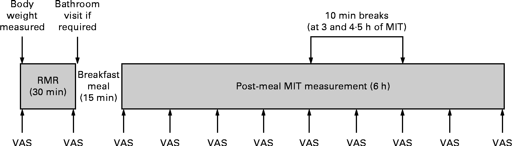
An overview of the protocol for test days 2 and 3 is shown in Fig. 1. Upon arrival at the laboratory, body weight was measured and then the RMR was measured in a fasted state for 30 min. This RMR measurement served as the ‘baseline’ energy expenditure for the calculation of MIT. Immediately after this baseline RMR measurement, the participants consumed a fixed test meal within 15 min. The metabolic measurement was then resumed, and postprandial energy expenditure was measured for a total of 6 h, with two 10 min ‘comfort breaks’ at 3 and 4·5 h. These breaks were mandatory, and all the participants were required to walk along the corridor to the restrooms on both test days 2 and 3. For all metabolic measurements, the participants were in a semi-reclined position in a lounge chair and the position of the participants was consistent between the test days. Before commencing the pre-meal RMR measurement, before and after breakfast, and then at 45 min intervals during the 6 h postprandial measurement period, the participants rated their subjective alertness and comfort sensations using visual analogue scales (VAS). This was done to evaluate the levels of restlessness and alertness both throughout the tests and between the days to consider their contribution to MIT variability. The participants were able to watch movies for the duration of the metabolic measurement period.

Fig. 1 Procedure for meal-induced thermogenesis (MIT) test days. The visual analogue scale (VAS) ratings were administered at 45 min intervals throughout the testing.
Test meal composition
The standard fixed breakfast meal on test days 2 and 3 represented a typical breakfast and consisted of muesli with milk, toast with margarine and jam, and a glass of orange juice. The meal provided 2410 kJ and comprised 20·1 g of fat, 78·2 g of carbohydrate and 20·6 g of protein, giving relative energy contributions of 32 % fat, 54 % carbohydrate and 14 % protein, respectively.
Measures of resting and postprandial energy expenditure
Resting and postprandial energy expenditure was measured using indirect calorimetry with a ventilated hood and canopy system (TrueOne 2400; Parvo Medics). The rate of flow of air being pumped through the hood was manually adjusted to maintain a constant CO2 level in the hood between 1·00 and 1·20 %. O2 concentration in the hood was measured with a paramagnetic oxygen analyser, and CO2 concentration was measured with an IR single-beam single-wavelength CO2 analyser. O2 consumption and CO2 production were calculated as the difference between the expired air in the hood and room air. Energy expenditure was calculated automatically using the TrueOne 2400 Metabolic Measurement System OUSW 4.3 software (Parvo Medics) from VO2 and VCO2 measured continuously throughout the testing using the Weir formula, which calculates the non-protein energy equivalent for O2(Reference Weir27):
 $$\begin{eqnarray} Energy\,expenditure\,(kJ) = ((1\cdot 106\times RER) + 3\cdot 941)\times VO_{2}\times 4\cdot 184. \end{eqnarray}$$
The metabolic cart was calibrated before each measurement period for flow, using a standard 3-litres calibration syringe and gas concentration using a two-point calibration procedure using room air and a standardised calibration gas (16·0 % O2, 1·0 % CO2). To control for any drift within the gas analysers, automated 30 s calibrations were performed at 5 min intervals throughout the measurement period.
Data handling and calculations
Pre-meal RMR
To ensure that the pre-meal RMR was measured during a stable period, the initial 10 min of the 30 min RMR measurement were discarded, and the RMR was calculated as the lowest 10 min average during the final 20 min of the 30 min measurement period. The CV for VO2 over the final 20 min of the tests averaged 5 (sd 2) %. Estimated RMR were calculated for each participant using the Schofield equations based on height and body weight(28) to determine whether the measured RMR were consistent with the predicted values of RMR.
Postprandial energy expenditure
Data from the 6 h postprandial measurement period were averaged over 15 min intervals and plotted against time. To minimise the effect of movement on the measurement of energy expenditure, the first 5 min of the postprandial measurement (i.e. immediately following breakfast) and 5 min periods following each of the prescribed breaks at 3 and 4·5 h were excluded from the calculations. The peak postprandial energy expenditure was defined as the 15 min interval with the highest rate of energy expenditure, and the time of peak was defined as the time that corresponded with this 15 min maximum. MIT on each test day was calculated as the energy expenditure above the RMR. This was calculated by averaging all the postprandial 15 min data points where the rate of energy expenditure was greater than that during the baseline RMR measurement, subtracting RMR and then multiplying the ‘net’ energy expenditure by the time taken for energy expenditure to return to the baseline RMR for a minimum of 30 min. MIT was also expressed as a percentage of the total energy of the test meal. To minimise the effect of day-to-day variability in RMR on the calculation of MIT, MIT was also calculated for both test days using the lower of the two pre-meal RMR measured on test days 2 and 3 (a ‘fixed’ baseline). The lowest RMR was chosen as it was considered to represent the participants in their most rested state and more likely to reflect their RMR after prolonged resting during their MIT measurement. RMR sdwas calculated over the 10 min period used for each participant's RMR measurement. The MIT responses of the participants were considered to have returned to the baseline if their energy expenditure returned to within 1 sd of their RMR for a minimum of 30 min.
Subjective ratings of alertness and comfort
Questions were administered on a laptop to measure the subjective ratings of alertness and comfort using VAS. The participants were asked to rate their intensity of alertness and comfort by moving a cursor along a 100 mm continuous line on a laptop with the two extremes of each question at either end. The questions asked included ‘How content are you right now?’, ‘How alert are you right now?’, ‘How comfortable are you right now?’ and ‘How great is your desire to move right now?’. The minimum and maximum VAS scores were 0 and 100 mm, respectively.
Calculation of visual analogue scale ratings
The subjective alertness and comfort sensations were expressed in millimetres and calculated by averaging the VAS scores from each 45 min period after the ingestion of the fixed meal.
Statistical analysis
SPSS version 18 for Windows (SPSS, Inc.) was used for the statistical analysis. A value of P< 0·05 was considered statistically significant. All values are reported as means and standard deviations. Data were verified as normally distributed using Shapiro–Wilk tests of normality before the analysis. A repeated-measures ANOVA was used to test for changes in body weight between the days, and a one-way ANOVA was used to compare the differences in characteristics and RMR between males and females. To determine the extent to which the measured RMR varied from the Schofield predictions, the measured RMR were subtracted from the predicted RMR and expressed as a percentage difference from the predicted RMR. Paired t tests were used to determine significant differences between the predicted and measured RMR. To assess for the reproducibility of the response curve, the cumulative MIT at 3, 4 and 5 h were calculated and expressed as a percentage of the MIT measured at 6 h. Paired t tests were used to assess for any significant changes in the peak postprandial energy expenditure (kJ) and the time of this peak. Paired t tests and CV were used for determining differences between the days and the variability of the pre-meal RMR, MIT in both absolute terms (total energy (kJ) over the time period) and relative terms (the proportion of the total response completed in the time period), and MIT (calculated with the ‘fixed’ baseline method). A Bland–Altman plot was used to depict the mean difference and 95 % limits of agreement in the MIT response between the days. A paired t test was used to compare the CV of the standard MIT calculation method and that of the ‘fixed’ baseline calculation method, and a repeated-measures ANOVA was used to compare the CV between the MIT calculated after 3, 4, 5 and 6 h. Minimal detectable change (MDC), which is defined as the minimal amount of change that is not due to the variation in measurement noise(Reference Steffen and Seney29), was calculated for MIT. Scores at or above the MDC level can be attributed to the intervention rather than to the measurement error. The measurement error includes the expected or typical variability in the physiology of the participants over repeated tests where tests are undertaken under the same conditions(Reference Steffen and Seney29). MDC scores were calculated for MIT using the following formula:
 $$\begin{eqnarray} MDC_{90} = sem\times 1\cdot 65\times \surd 2, \end{eqnarray}$$
where sem is calculated using the following equation(Reference Steffen and Seney29, Reference Ries, Echternach and Nof30):
 $$\begin{eqnarray} sem = sd\times \surd (1 - r ). \end{eqnarray}$$
In these equations, sd is the standard deviation of the measure, r is the intra-class correlation coefficient for the subject group, 1·65 represents the z-score at the 90 % CI and 1·65 is multiplied by the square root of 2 to account for errors associated with repeated measures. Pearson's correlations were used to assess the relationship between the MIT (kJ) calculated at 3, 4 and 5 h and the response measured at 6 h. A 2 × 2 repeated-measures ANOVA with the test day and each 45 min VAS rating as repeated measures was used to determine differences in the VAS variables between the days and changes in the VAS variables across the MIT test duration, and CV was used to determine the VAS between-day variability. The CV was calculated to determine the variability of the fasting, average postprandial and peak postprandial RER. Pearson's correlations were used to determine any relationship between MIT and RER and MIT and RMR.
Results
Table 1 provides the characteristics of the participants. Compared with females, males were heavier and taller, but these differences did not reach statistical significance. Furthermore, males and females did not differ significantly in terms of age, BMI or percentage fat mass. The participants maintained a stable weight across the study period (day 1: 65·2 (sd 11·3) kg, day 2: 65·1 (sd 11·2) kg, and day 3: 65·2 (sd 10·7) kg; P =0·87). There were no differences between the RMR determined as the lowest 10 min average and the predicted RMR using the Schofield equations on either test day 1 (measured RMR 1·1 (sd 8·9) % below the predicted RMR; P= 0·72) or test day 2 (measured RMR 0·9 (sd 11·3) % above the predicted RMR; P= 0·77).
Table 1 Descriptive characteristics of the participants (Mean values and standard deviations)

% FM, percentage of fat mass; DXA, dual-energy X-ray absorptiometry.
* P values for comparisons between the male and female participants.
† RMR was calculated as the average pre-meal RMR of both test days.
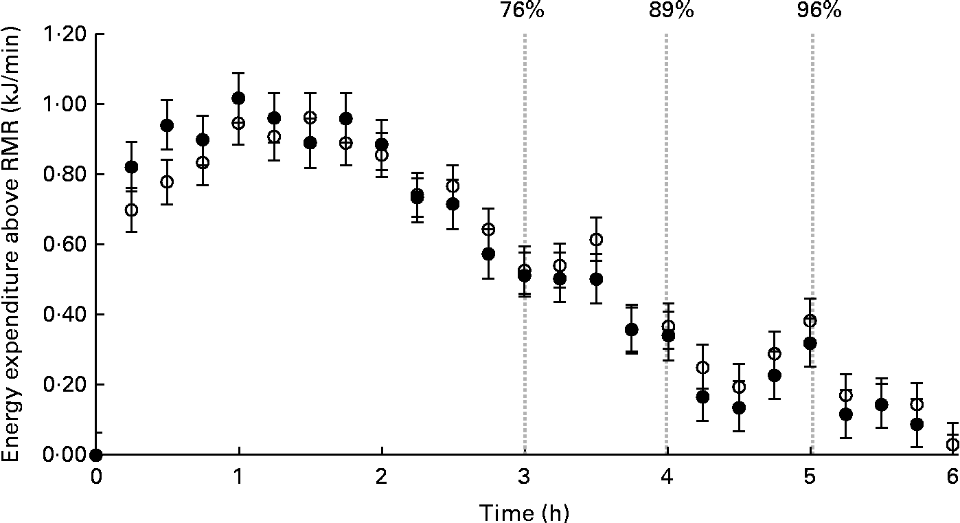
Fig. 2 illustrates the average MIT response for MIT1 and MIT2. The participants' peak rates of energy expenditure above RMR were similar between the tests (MIT1: 1·09 (sd 0·28) kJ/min v. MIT2: 1·15 (sd 0·47) kJ/min; P =0·64). Although the peak tended to occur earlier for the participants during MIT1 than during MIT2, this difference was not significant (MIT1: 68 (sd 38) min v. MIT2: 95 (sd 55) min; P =0·31). At the end of the 6 h measurement period, energy expenditure returned to the baseline (i.e. within 1 sd of the pre-meal RMR) for six participants during MIT1 and six participants during MIT2. Five of these were the same participants. For the remaining participants, the average energy expenditure over the final 30 min of the measurement period averaged 0·46 (sd 0·25) kJ/min above the baseline.
Fig. 2 Average meal-induced thermogenesis (MIT) response. MIT1 is shown as ○ and MIT2 is shown as ●. Data points are representative of 15 min averages of energy expenditure post-meal consumption above the baseline RMR (kJ/min). The first data point for each series represents the pre-meal RMR. MIT was calculated as the total energy expenditure above RMR until energy expenditure returns to the RMR value. Values are means, with their standard errors represented by vertical bars. The percentage of the 6 h response completed after 3, 4 and 5 h was 76, 89 and 96 %, respectively, as illustrated in the graph.
The cumulative MIT completed within 3, 4 and 5 h was calculated for MIT1 and MIT2 and expressed as a percentage of the MIT response measured at 6 h for each test (Table 2). On average, the proportion of the response completed at 3, 4 and 5 h was 76, 89 and 96 %, respectively. The between-day variability of the percentage of the 6 h response completed within 3, 4 and 5 h is provided in Table 2.
Table 2 Meal-induced thermogenesis (MIT) calculated after 3, 4, 5 and 6 h and the percentage of the 6 h MIT complete within 3, 4 and 5 h* (Mean values and standard deviations)

* MIT is reported in both absolute terms (kJ above RMR) and as a percentage of the test meal. Percentage MIT completed is expressed as a percentage of the 6 h MIT measurement. CV of the total MIT between days and the CV of the percentages of the 6 h MIT compete within 3, 4 and 5 h between days are also provided.
With respect to the reproducibility of the MIT response, the pre-meal RMR was not significantly different between the days (MIT1 RMR: 4·52 (sd 0·84) kJ/min; MIT2 RMR: 4·60 (sd 0·88) kJ/min; P =0·66). The mean between-day CV was 9 (sd 6) %. As outlined in Table 2, there was no significant difference in the total MIT response between the days (P =0·83) and the CV was significantly lower at 3 and 4 h than at 6 h (3 v. 6 h CV: P =0·02; 4 v. 6 h CV: P =0·03).
To minimise the potential effect of between-day variability of RMR on variability in MIT, both MIT1 and MIT2 were also calculated using a ‘fixed’ RMR value (the lower of the two pre-meal RMR) for each participant. Using this approach, the between-day CV for the 6 h measurement was 33 (sd 12) %, which was not significantly different from that of the standard approach (P =0·98).
The individual between-day differences are illustrated with a Bland–Altman plot in Fig. 3. While the mean difference between the days was − 9 kJ ( − 0·4 %; P =0·83), the 95 % limits of agreement were wide, ranging from 239 to − 257 kJ (9·9–10·7 % of energy intake). However, as shown in Fig. 3, this large between-day difference was heavily influenced by two individuals who experienced marked differences (+236 kJ (9·8 %) and 246 kJ (10·2 %)) between MIT1 and MIT2. The remaining eight participants had between-day differences in MIT within ± 87 kJ (3·2 % of energy intake). While there was no clear reason for excluding data from these two participants from the analysis, calculations performed without these two responses resulted in a similar mean between-day difference of − 10 kJ ( − 0·4 %), but reduced the 95 % limits considerably to between 115 and − 135 KJ (4·8 to − 5·6 %). Day-to-day variability determined using the intra-class correlation coefficient was 0·382. MDC90 was calculated as 122·1 kJ.

Fig. 3 Bland–Altman plot of individual differences in meal-induced thermogenesis (MIT) (kJ) between MIT1 and MIT2. —— indicates mean bias and - - - represents the upper and lower 95 % limits of agreement. The upper 95 % limit of agreement was 239 kJ and the lower 95 % limit of agreement was − 257 kJ. The mean difference was − 9 kJ. Difference calculated as MIT1 minus MIT2. Males are shown as ● and females are shown as ▲.
The relationship between the MIT measured for 6 h and the cumulative MIT values measured after 3, 4, and 5 h is illustrated in Fig. 4. The MIT measured after 3, 4 and 5 h was strongly correlated with the MIT measured over 6 h during both MIT1 and MIT2 (correlations reported in Fig. 4).

Fig. 4 Regression line of the meal-induced thermogenesis (MIT) (kJ) measured over (a) 3, (b) 4 and (c) 5 h compared with the MIT measured over 6 h. MIT1 is shown as ○ and MIT2 is shown as ●. The correlation coefficients are as follows. (a) MIT1: R 0·992, P< 0·001; MIT2: R 0·958, P< 0·001. (b) MIT1: R 0·998, P< 0·001; MIT2: R 0·990, P< 0·001. (c) MIT1: R 0·996, P< 0·001; MIT2: R 0·997, P< 0·001.
Despite a large variation in the MIT response between the days, the between-day CV for the VAS variables was relatively low. There were no significant differences in contentment (P =0·68), level of comfort (P =0·14) or desire to move (P =0·60) between the days, with between-day CV of 11, 10, and 11 %, respectively. Although the level of alertness was significantly higher in MIT2 than in MIT1 (P =0·04), the between-day CV was only 7 %. Ratings of alertness did not change across the duration of the tests (P =0·93). However, there was a significant decrease in contentment and comfort and a significant increase in the desire to move over the 6 h postprandial measurement period (P< 0·001 for all variables). This was the result of significant changes over the first 3 h (all variables P< 0·001), with no significant changes being observed between 3 and 6 h (contentment: P =0·159; comfort: P =0·59; desire to move: P =0·80).
There were no between-day differences in the fasting RER (MIT1: 0·79 (sd 0·05); MIT2: 0·79 (sd 0·05); P =0·66), average 6 h postprandial RER (MIT1: 0·80 (sd 0·02); MIT2: 0·80 (sd 0·04); P =0·98) and peak postprandial RER (MIT1: 0·86 (sd 0·03); MIT2: 0·86 (sd 0·04); P =0·99). The between-day variability for these RER variables was low with CV of 5, 4 and 3 %, respectively. There was no relationship between MIT and average 6 h postprandial RER (MIT1: P =0·576; MIT2: P =0·334) or MIT and peak postprandial RER (MIT1: P =0·699; MIT2: P =0·622). Further analysis revealed no relationship between the size of the MIT response of the participants and their RMR (MIT1: P =0·319; MIT2: P =0·405).
Discussion
The primary findings from the present study were that the magnitude of MIT measured for 3, 4 or 5 h strongly correlated with that of the 6 h MIT and the proportion of the 6 h MIT response completed at 3, 4 or 5 h was reproducible between the days. In addition, while measurements made over shorter durations were more reproducible, using a ‘fixed’ RMR did not reduce the day-to-day variability in the measurements.
MIT is a small but important component of total daily energy expenditure. MIT is typically measured for up to 6 h(Reference Laville, Cornu and Normand4–Reference Bessard, Schutz and Jequier7), which places a large burden on the participant, and thus it is important to consider whether shorter measurement durations may be used. The initial few hours of the MIT measurement can provide a considerable amount of information about the total MIT response. In the present study, the peak postprandial energy expenditure occurred at 67 and 94 min in MIT1 and MIT2, respectively, which was within the range of 30–120 min reported previously in studies using similar-sized meals (2510–4054 kJ)(Reference Katzeff and Danforth9, Reference Dabbech, Boulier and Apfelbaum15, Reference Maffeis, Schutz and Grezzani31). Furthermore, 76, 89 and 96 % of the 6 h response was completed at 3, 4 and 5 h, respectively, which is similar to, albeit slightly higher than, the 60, 78 and 91 % reported by Reed & Hill(Reference Reed and Hill18) at the same time points. The inclusion of larger meals in the Reed & Hill study (2711–5807 kJ) compared with the 2410 kJ test meal in the present study may have contributed to this difference because larger meals may delay the peak response and lengthen the MIT total duration and therefore result in a greater proportion of the MIT occurring later in the measurement period(Reference Melanson, Saltzman and Vinken11, Reference Reed and Hill18, Reference Karst, Steiniger and Noack19).
The use of either a relative (to RMR) or a standard meal size remains equivocal. While several studies have used meals relative to body weight or RMR(Reference Nelson, Weinsier and James5, Reference Bessard, Schutz and Jequier7, Reference Leibel, Rosenbaum and Hirsch8, Reference Armellini, Zamboni and Mino24), a large number have provided meals of standard sizes for all participants(Reference Scott and Devore2, Reference Segal, Albu and Chun6, Reference Katzeff and Danforth9, Reference Tentolouris, Pavlatos and Kokkinos13, Reference Dabbech, Boulier and Apfelbaum15, Reference Scott, Fernandes and Lehman17, Reference Dabbech, Aubert and Apfelbaum20, Reference Houde-Nadeau, de Jonge and Garrel22, Reference Segal, Chun and Coronel26, Reference Maffeis, Schutz and Grezzani31). D'Alessio et al. (Reference D'Alessio, Kavle and Mozzoli12) compared four energetic loads in lean and obese individuals and found that MIT remained proportional to energy intake for each individual regardless of meal size, indicating that meal size is inconsequential when measuring the entire MIT response. However, as larger meals have been shown to prolong the MIT response(Reference Melanson, Saltzman and Vinken11, Reference Reed and Hill18, Reference Karst, Steiniger and Noack19), providing relative meal sizes may result in longer and more delayed responses in individuals with a greater body mass. This raises the concern of measuring different proportions of the total MIT response over a fixed measurement period, either between individuals or pre- and post-weight loss, unless the entire MIT response is measured. A standard meal size was chosen for the present study to minimise variation in the timing of the response in order to provide tighter estimates of the proportion of the chosen meal completed within 3, 4 and 5 h.
In the present study, the magnitude of MIT measured for 3, 4 and 5 h was strongly correlated with the 6 h measurement, which is also in line with previous findings(Reference Reed and Hill18). Furthermore, the proportion of the response completed at 3, 4 and 5 h was consistent between the days (Table 2), indicating that the temporal profile of the response is reproducible. As such, for an individual whose 6 h MIT response was smaller on one test day, his or her response was proportionally smaller at 3, 4 and 5 h. Hence, shorter measurement durations reflected the magnitude of each individual's total MIT and the proportion of his or her total response captured at these time points was comparable between the test days. This suggests that while measurement durations of approximately 6 h may be required to quantify the entire MIT response to a meal, shorter measures may provide sufficient information to perform between-group and within-subject comparisons across time. This assumes that the timing of the response is the same between the groups for the former and that the test meal (i.e. energy and composition) is held constant for the latter.
In the present study, MIT reproducibility was measured using two approaches. The CV was used to determine the variability relative to the size of the response to allow a comparison with previous studies, and a Bland–Altman plot with 95 % limits of agreement was used to illustrate the extent of individual between-day variation. Previously, studies measuring MIT with a ventilated hood and using the standard pre-meal RMR to calculate the response have reported average CV for MIT between 15 and 29 %(Reference Dabbech, Aubert and Apfelbaum20–Reference Piers, Soares and Maken23); however, CV as high as 42 % have been reported within some groups, even under highly controlled conditions(Reference Weststrate21). While there was no significant difference in the group MIT between the days (Fig. 2), there was a considerable within-individual variability with an average between-day CV of 33 % for the 6 h measurement, which is at the upper end of the previously reported range. Although the variability was significantly decreased when MIT was measured over 3 and 4 h, it was still 26–29 %. The reasons for the high CV in the present study are not clear, especially since consistent and standardised approaches were undertaken to minimise variability. Despite the between-day variability of MIT, the variability of the fasting RER, 6 h postprandial average RER and peak postprandial RER values was low. The low RER variability despite a much greater MIT variability is similar to previous findings(Reference Weststrate21, Reference Piers, Soares and Maken23) and indicates that while MIT may be greater on any particular test day, the substrates oxidised increase proportionally.
To minimise the effect of day-to-day differences in RMR and glycogen stores, both of which may affect the magnitude of the MIT response(Reference Acheson, Schutz and Bessard32), pre-test conditions were controlled, with the participants being asked to avoid exercise outside of their daily work requirements for a minimum of 48 h before the test days and to replicate their evening meal preceding both test days. Greater control of diet in the days preceding the measurements may have improved reproducibility. However, it seems unlikely that pre-test diet can explain the variability in MIT, given that Weststrate(Reference Weststrate21) found no improvement in the reproducibility of MIT even when controlling antecedent diet for 4 d before MIT measurements. Where facilities allow, accommodating participants at the testing centre on the night preceding their RMR and MIT tests may offer an additional means of minimising variability through more stringent control over activity and meal choices on the evening before, and morning of, the test days.
It is also critical to control conditions during the tests. Relative to total energy expenditure, MIT is small and is, therefore, easily obscured by any noise in the measure. Boredom and a lack of entertainment can increase restlessness and fidgeting(Reference Calabro, Welk and Silva33), and this may ‘artificially’ increase RMR(Reference Dietz, Bandini and Morelli34) and contribute to variability during the measurements(Reference Calabro, Welk and Silva33). In the present study, the participants were able to watch movies of their choice for the duration of the measurement period and were provided with two opportunities for brief breaks during the measurement period. Despite this, the participants became more restless over the 6 h measurement period, with significantly lower ratings of contentment and comfort and significantly higher ratings of desire to move at 3 and 6 h than at the start of the measurement period. It is worth considering how this may affect the measured response within a test and the day-to-day variability. While energy expenditure had returned to the baseline in six of the ten participants by 6 h, it remained slightly elevated in the remaining four. While this may represent a true biological response in these individuals, it is also possible that increased restlessness in the latter parts of the tests contributed to the sustained elevation in the metabolic rate. On the other hand, given that the between-day CV for all these variables was between 7 and 11 % and, with the exception of alertness, there were no significant differences between the test days, differences in comfort or the level of arousal are unlikely to explain the high day-to-day variability in MIT.
While eight of the ten participants had differences in MIT values within 115 and − 135 kJ between the two tests, the remaining two participants had very large between-day differences (Fig. 3). Both participants were female, and because some females were tested in different phases of the menstrual cycle, this may have contributed to the large differences. However, Melanson et al. (Reference Melanson, Saltzman and Russell35) compared women in the luteal and follicular phases of their menstrual cycle and reported no differences in the MIT between the two phases. Furthermore, while one of the participants with high between-day differences was in different phases of the menstrual cycle for the two MIT tests, the other was in the luteal phase on both test days, suggesting that the large day-to-day variability was not due to the menstrual cycle alone. In addition, both participants complied with the pre-test meal and exercise requirements, and there were no further obvious reasons for their variability.
The between-day CV for RMR was 9 % in the present study, and while this may have contributed to the between-day variability of MIT, the use of a ‘fixed’ RMR did not result in a reduction in variability. This is in contrast with previous research in which the use of a ‘fixed’ RMR had resulted in a significant reduction in the day-to-day variability(Reference Dabbech, Aubert and Apfelbaum20, Reference Piers, Soares and Maken23). A possible explanation for this discrepancy is the method used to calculate CV. In studies reporting that the use of a fixed RMR improved reproducibility, the fixed RMR has tended to produce substantially higher MIT values. Because the same absolute between-day difference in MIT (e.g. 60 kJ) will result in a smaller CV with large MIT values (e.g. test 1: 170 and test 2: 230 kJ; CV: 21 %) compared with small MIT values (e.g. test 1: 70 and test 2: 130 kJ; CV: 42 %), the apparent improvement in MIT with a ‘fixed’ RMR may be more a mathematical function rather than a reflection of a true reduction in biological variability between the days.
It is important to note that the findings from the present study apply to this ‘typical’ mixed breakfast meal (2410 kJ: 20·1 g fat, 78·2 g carbohydrate and 20·6 g protein) with a relative energy contribution of 32 % fat, 54 % carbohydrate and 14 % protein. In situations with a markedly different meal composition, there is the possibility of an altered temporal function of gastric transit and therefore MIT(Reference Tentolouris, Pavlatos and Kokkinos13, Reference Scott, Fernandes and Lehman17, Reference Karst, Steiniger and Noack19). A limitation of the study was the small sample size with ten participants underpowered to be able to determine significant differences. However, the data from the present study allow the determination of variability and measures of MDC to inform future studies. Based on the findings from the MDC90, we may suggest that a difference of ≥ 122 kJ between the test days would be required to be confident that the difference was from the intervention rather than from measurement variability. Retrospective power calculations indicated that to detect a difference of 9 kJ, as was the average difference between the days in the present study, a sample of 1567 participants would have been required. While the small sample size in the present study may not provide a population-wide example of intra-class correlation coefficient and variability for calculating MDC90, the present study does suggest that the differences that were noted between the days would not have been found to be statistically significant in most experimental or clinical studies. Should the study of 1567 participants be undertaken, based on the results from the present study, Cohen's d calculation of effect size 0·08 indicates that the difference is trivial, even if it would reach statistical significance. Additionally, while the homogeneity of the study population limits the findings to those with similar characteristics, the advantage is the ability to provide a standardised test meal to all the participants and therefore provide tighter guidelines on the time requirements for MIT measurement for an average-sized meal. However, some research has indicated a delayed MIT response in obese individuals(Reference D'Alessio, Kavle and Mozzoli12, Reference Reed and Hill18, Reference Segal, Chun and Coronel26). Therefore, further research is necessary to determine the proportion of MIT captured within shorter measurement durations in a wider range of individuals including obese individuals and in a larger variety of meal compositions.
In conclusion, the proportion of the total MIT measured over 3, 4 or 5 h is reproducible between days and the magnitude of the response measured over shorter durations is strongly related to the magnitude of an individual's total response. Furthermore, important elements of the response, for example the peak in energy expenditure, occur early in the measurement period, and thus measurements as short as 3 h provide valuable information about an individual's response to meal ingestion. Therefore, given the substantial participant burden and potential for the confounding effects of restlessness associated with long measurement durations, shorter measurement durations may provide a practical option for repeated measurements of MIT. Given that factors such as body weight, meal size and meal composition may alter the timing of the MIT response curve(Reference Melanson, Saltzman and Vinken11–Reference Tentolouris, Pavlatos and Kokkinos13, Reference Reed and Hill18, Reference Karst, Steiniger and Noack19), further investigation is recommended to determine the applicability of shorter measurement durations in a wider population and for different meals.
Acknowledgements
The present study received no specific grant from any funding agency in the public, commercial or not-for-profit sectors. The contributions of the authors are as follows: L. C. R.-C., R. E. W., N. M. B. and N. A. K. were involved in the conception and design of the study; L. C. R.-C. was responsible for data acquisition and statistical analysis; L. C. R.-C. and R. E. W. were involved in the writing of the manuscript. All authors contributed to the study interpretation, reviewing of each draft of the manuscript, the decision of the final content and the approval of the final manuscript. None of the authors has any personal or financial conflicts of interest.