


Settings and sample
We focus on two centers located in the northwest Peten, Guatemala. This region is an ecotone, grading gently from east to west (Figure 1). Its eastern extreme, around the Late Preclassic and Early Classic center of Achiotal, is part of a karst margin plain that defines the western part of the Peten Plateau. Its western extreme is part of the Laguna del Tigre wetlands, characterized by many small freshwater lagoons and small perennial surface streams. La Corona is positioned at the point of transition between these two landscapes. The entire region is exceedingly flat, with limited surface drainage.
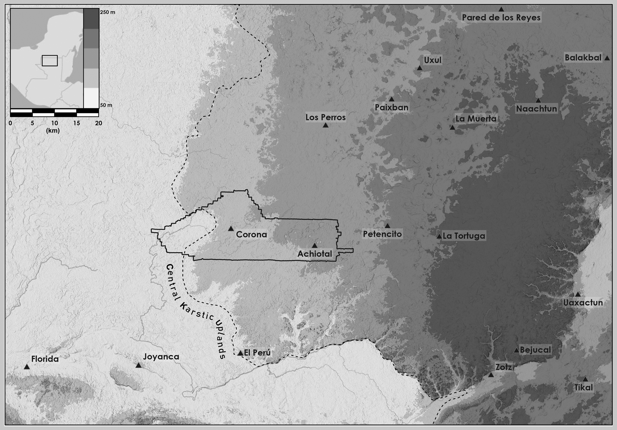
Figure 1. Maya sites in northwestern Peten, along with the boundaries of the ALS capture.
Though remote, La Corona was peppered with sculpted monuments that recorded its political association with the important Classic Maya dynasty of Kaanul, the hegemonic rulers of the Classic period centers of Dzibanche and Calakmul with which it maintained a close alliance for over two centuries in the Late Classic period (Baron Reference Baron2016; Canuto and Barrientos Q. Reference Canuto, Barrientos Q., Houk, Arroyo and Powis2020; Lamoureux-St-Hilaire et al. Reference Lamoureux-St-Hilaire, Canuto, Christian Wells, Cagnato and Barrientos Q.2019; Martin Reference Martin, Inomata and Houston2001:183, Reference Martin2008; Stuart et al. Reference Stuart, Canuto, Barrientos Q. and González2018). Despite this important role as a tightly integrated but geographically distant political dependency, La Corona's civic-ceremonial core was small (~1 km2), composed of two main architectural complexes, interspersed with a handful of minor shrines and residential clusters (Barrientos Q. et al. Reference Barrientos Q., Canuto, Baron, Desailly-Chanson, Love, Arroyo, Aragón, Palma and Arroyave2011). Moreover, initial mapping, survey, and reconnaissance efforts indicated that the surrounding region was sparsely settled (Canuto et al. Reference Canuto, Guenter, Tsesmeli and Marken2005; Chiriboga Reference Chiriboga, Canuto, Barrientos Q. and Ponce2013; Guzmán Piedrasanta Reference Guzmán Piedrasanta, Canuto, Barrientos Q. and Ponce2012; Marken Reference Marken, Canuto and Q.2010).
In 2016, the Pacunam LiDAR Initiative (PLI) undertook a 2,144 km2 airbone lidar scanning (ALS) survey of the Central Maya Lowlands in northern Guatemala (see Canuto et al. Reference Canuto, Estrada-Belli, Garrison, Houston, Acuña, Kováč, Marken, Nondédéo, Auld-Thomas, Castanet, Chatelain, Chiriboga, Drápela, Lieskovský, Tokovinine, Velasquez, Fernández-Díaz and Shrestha2018, for details on PLI). Data were collected by the National Center for Airborne Laser Mapping (NCALM), which produced digital terrain models with a 1 m grid resolution. Proyecto Regional Arqueológico La Corona (PRALC) provided a 432 km2 block of LiDAR data that present the singular opportunity to study how a small Late Classic center of outsized political importance correlates with a sparse population (Figure 1).
In this study, we pose the question of how the application of the Gini coefficient can help further illuminate the nature of La Corona as a small subordinate center. Would its populations reflect a degree of inequality as acute as that of those populations living in the shadows of larger political centers such as Dzibanche or Calakmul? How would the Late Preclassic populations located further east compare with their Classic period successors?
Settlement density and typology
Heads-up digitization iterating with field validation resulted in the identification of 3,853 structures and 10 small centers, suggesting that the Late Classic population of the region was around 12,000 people, with an overall population density of less than 0.5 people/ha—sparse by Lowland Maya standards (see Culbert and Rice Reference Culbert and Rice1990). Assessing the distribution of settlement throughout the survey domain demonstrated that much of the region was nearly vacant, while the rest had less than 60 structures/km2, a measure often interpreted as indicating “rural.” At the opposite end of the density spectrum, the region's highest recorded density was 227 structures/km2, a value that characterizes a small ~100 ha area within the La Corona polity core. Relative to the rest of the Peten, in which Lowland Maya monumental centers reach settlement densities above 300 structures/km2, even La Corona's densest area registers as both small and low.
The region's flat, ecotonal setting leaves it with a paucity of preferred landforms relative to the rest of the Maya lowlands (see Canuto and Auld-Thomas Reference Canuto and Auld-Thomas2021). For instance, the highly preferred ridge and islote landforms comprise only ~19 percent of the whole area. Yet these landforms contain nearly 90 percent of its settlement, resulting in a productive density of ~56 structures/km2. Even so, in adjacent parts of the Maya Lowlands, the settlement densities of preferred landforms are three to six times greater than those of the Corona region. Overall, these various assessments leave us with one inescapable conclusion: by any reasonable measure, the “Corona community” is indeed less dense than the rest of the Central Maya Lowlands, in both absolute and relative terms.
Before we turn to our Gini results, we focus on our settlement typology to further clarify the kind of settlement and populations that inhabited this region. Settlement classification and field verification efforts centered around the monumental cores of La Corona, Achiotal, and Chable (Canuto and Auld-Thomas Reference Canuto, Auld-Thomas, Barrientos Q., Canuto and López2020, Reference Canuto and Auld-Thomas2021). To date, PRALC's field validation has conducted full-coverage survey of ~23.5 km2 throughout the region, which has demonstrated excellent fidelity between what we identified through heads-up digitizing and what we encountered on the ground (single-pass assessment: 0.908 user accuracy; 0.752 producer accuracy; 0.823 F1-score; Canuto and Auld-Thomas Reference Canuto and Auld-Thomas2021; see also Garrison et al. Reference Garrison, Thompson, Krause, Eshleman, Fernandez-Diaz, Dennis Baldwin and Cambranes2022). It has also allowed us to develop a locally parameterized settlement typology with a robust local sample.
Field validation showed that our digitizing was conservative, with false negatives outnumbering false positives. This is highly relevant to our purpose here, because “false negatives” were, overwhelmingly, small buildings. If there were a way to reliably account for them in our calculations, our derived Gini coefficient would be higher, since the additional small buildings would not be offset by the addition of midsize or large buildings, all of which were reliably identified in the LiDAR data.
Our survey defined a “group” as any set of archaeological features located within 35 m of one another (see Ashmore et al. Reference Ashmore, Connell, Ehret, Gifford, Theodore Neff, Vandenbosch, Leventhal and Ashmore1994; de Montmollin Reference de Montmollin1985). With ALS data, we quantified each structure's proximity relationships, demonstrating that over 85 percent of structures were located within 35 m of one another, thus buttressing our initial spatial definition of a group. We then classified each group into six categories, based on: number of mounds, mound height, presence of focal mound or patio within the group, and overall spatial arrangement (Figure 2). Notably, settlement in our study area consists of a hodge-podge of single mounds, informal clusters of buildings, formal patios, and so on, implying that the region's population was predominantly organized into single (multigenerational) family households. Basal platforms and clearly defined patios are both uncommon; instead, single mounds and irregular clusters of buildings represent some 40 percent of the dataset.
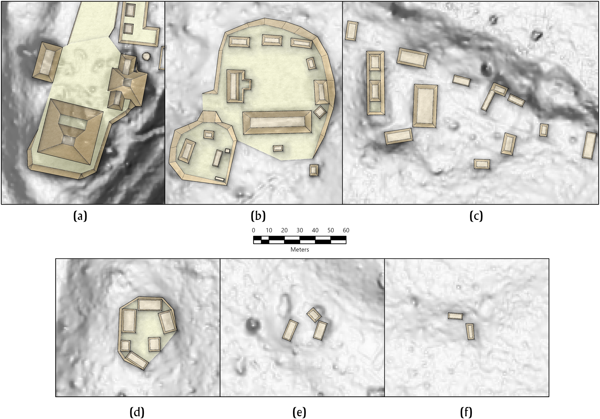
Figure 2. Settlement typology: (a) monumental core; (b) plaza; (c) patio cluster; (d) patio; (e) aggregate mound; and (f) single mound.
In our typology, the smallest unit (Type I) is the isolated mound; it represents a significant portion (~30 percent) of all settlement. Single buildings have long been regarded by some Mayanists as non-permanent or secondary residences, drawing on the ethnographic analog of “field houses,” used by Maya farmers to be close to their outfields during busy agricultural seasons (Ford Reference Ford1986; Horn III et al. Reference Horn, Tran and Ford2023; Sanders Reference Sanders and Ashmore1981). We do not dispute this argument; in fact, our own excavations support the idea that some isolated buildings in our region were not permanent homes. However, this analogy does not explain single mounds located within communities, which would not be the settings for outfield agriculture. Since most of our isolated mounds were located near other residential groups, it is unlikely that all were field houses or temporary shelters. Perhaps adjacent to now-invisible perishable structures, some Type I groups were nuclear family residences. Nevertheless, a key feature of the settlement in this area is the frequent occurrence of Type I (single mounds) not associated with any other buildings. Since these Type 1 buildings represent 10 percent of our total number of structures, how we handle them has a major impact on our Gini estimates.
Clustering methods
To calculate Gini coefficients for our area, we delineated groups beyond ground-truthing. To do so, we first identified each structure within our area of interest with a point using heads-up digitization. We then turned to a combination of two density-based spatial clustering algorithms—DBSCAN (ArcGIS Pro, 40 m search radius, with a minimum of two structures) and HDBSCAN (ArcGIS Pro, with a minimum of two structures)—which identify clusters among a set of unevenly distributed points within a given area; in this way, both tools are well-suited to the characteristic patchiness of Maya settlement. Both these tools resulted in the identification of point clusters of, at minimum, two buildings. We used both approaches: (1) to confirm the validity of one tool's clusters with those of the other; and (2) to provide alternative clusterings when one tool produced a cluster that did not meet our expectations of single household units.
After reviewing and confirming the clusters, we qualitatively eliminated clusters according to strict functional criteria. Our analysis eliminated a handful of complexes in the entire Corona-Achiotal region as categorically non-residential and disarticulated from a household. We also excluded a complex of two conical mounds north of La Corona, which are formally distinct, clearly not residential, and not contemporaneous with the rest of the Corona-Achiotal region's settlement system.
Returning to the thorny problem of “single mounds”, they are of no small consequence for estimations of inequality in Maya society. Excluding them altogether would risk artificially flattening Maya society, excluding the poorest people from analysis. But if the single mounds are secondary residences, to whom should they be attributed in the calculations? To deal with these two problems, we invoked spatial relationships. Single mounds within communities—where there would be no advantage to building a rancho for agricultural convenience—are included as genuine standalone houses. Single buildings that occur outside of communities are excluded from the analysis under the assumption that they mostly represent non-permanent dwellings. That these mounds are universally small and shabby, rarely more than 25 m2 or 30 cm high, means that they would contribute little in the way of area or volume to their owners’ architectural assets.
To distinguish which single mounds should be considered part of a household, despite their remoteness from the cluster, from those single mounds which should be excluded from our calculations as solitary “field” structures, we calculated the distance between each solitary (non-clustered) structure and its nearest cluster. We then compiled these nearest distances and, based on the overall distribution of nearest distances, identified 221 m as a threshold. In other words, there appeared to be a natural break in the distribution of distances of solitary buildings from cluster centers at approximately 220 m, suggesting that beyond that distance, solitary structures may have had a different function—that is, non-residential—relative to their closest residential cluster.
Scenarios
We calculated Gini coefficients (see Table 1) using both area and volume measurements as our “inequality metric” for four different analytical units. We did this to see what variations would result using different metrics as well as analytical units. In the first scenario we used only “individual residential structures,” as adopted by colleagues in Belize (Thompson et al. Reference Thompson, Feinman, Lemly and Prufer2021b). Only residential structures were used, and among those, only the ones measuring 20–275 m2 (see Thompson et al. Reference Thompson, Chase and Feinman2023). Single, isolated mounds were included in this scenario. The Gini coefficients were 0.34 for area and 0.59 for volume, with confidence intervals of less than 0.02 (Figure 3). For our second scenario, we aggregated (summed) all the structures within plazuela groups (Thompson et al. Reference Thompson, Feinman and Prufer2021a). In our case, these plazuela groups were the clusters that we had defined earlier, using a combination of HDBSCAN and DBSCAN. The Gini coefficients in this case were 0.44 for area and 0.69 for volume, with confidence intervals of less than 0.06 (Figure 4). A third version of this analysis took as its unit of analysis the entire plazuela group, aggregating structures and the basal platform where present. In our case, when our plazuela clusters had no basal platform, only the sum of the constituent structures was used (as in Scenario 2). That is, we did not include the area between structure mounds in the Gini calculation; given the irregular nature of many groups in our sample, doing so would have spuriously incorporated a great deal of natural topographic variation. The Gini coefficients were 0.53 for area and 0.69 for volume, with confidence intervals of less than 0.07 (Figure 5).
Table 1. Gini coefficients of four different scenarios.
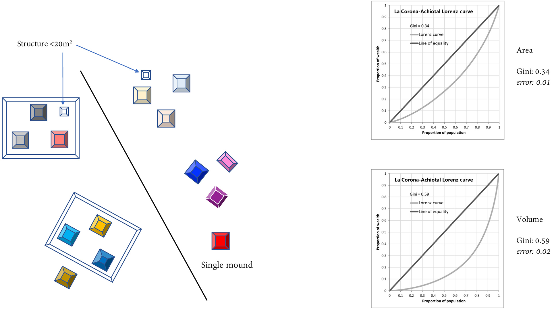
Figure 3. Gini coefficient: individual residential structures (20–275 m2, sample size: 3,363; Scenario 1).
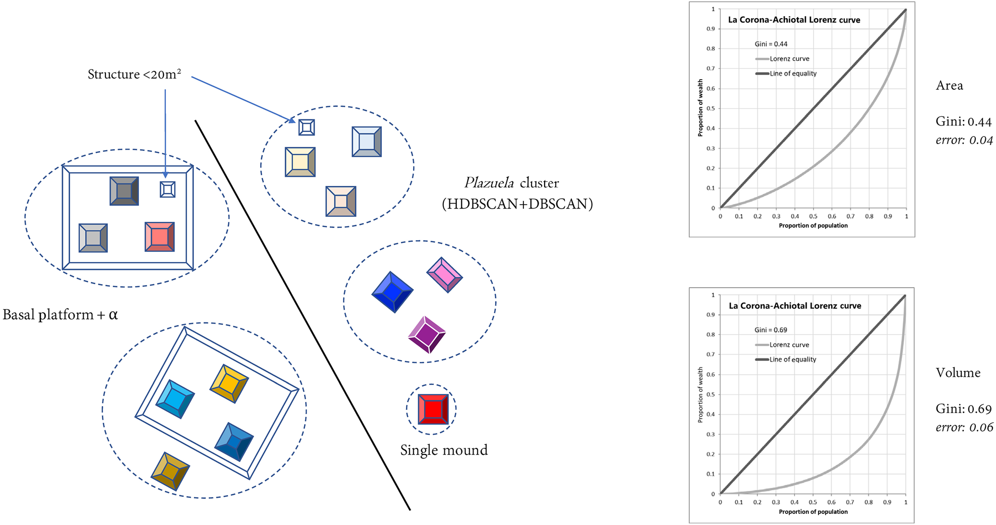
Figure 4. Gini coefficient: structures in plazuela groups (sample size: 985; Scenario 2).
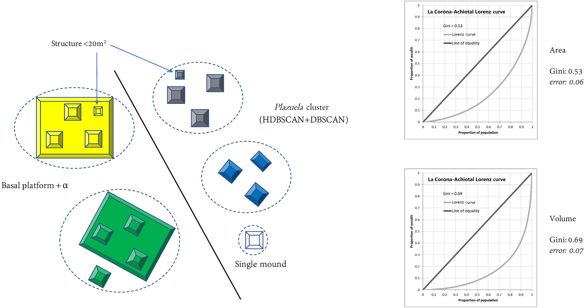
Figure 5. Gini coefficient: plazuela group, including basal platform (sample size: 978; Scenario 3).
For our fourth scenario, we return to the issue of single mounds. As noted above, we reasoned that single mounds (20–275 m2) in close spatial proximity to other multi-building clusters represent true residences. Therefore, in our fourth scenario, we included all single mounds within 221 m of another cluster and excluded all those that fell outside this distance as probable non-dwellings. We chose this distance because the distribution of single structures clustered either within 221 m or far beyond it. This calculation resulted in Gini coefficients that were 0.58 for area and 0.71 for volume, with confidence intervals of less than 0.06 (Figure 6).
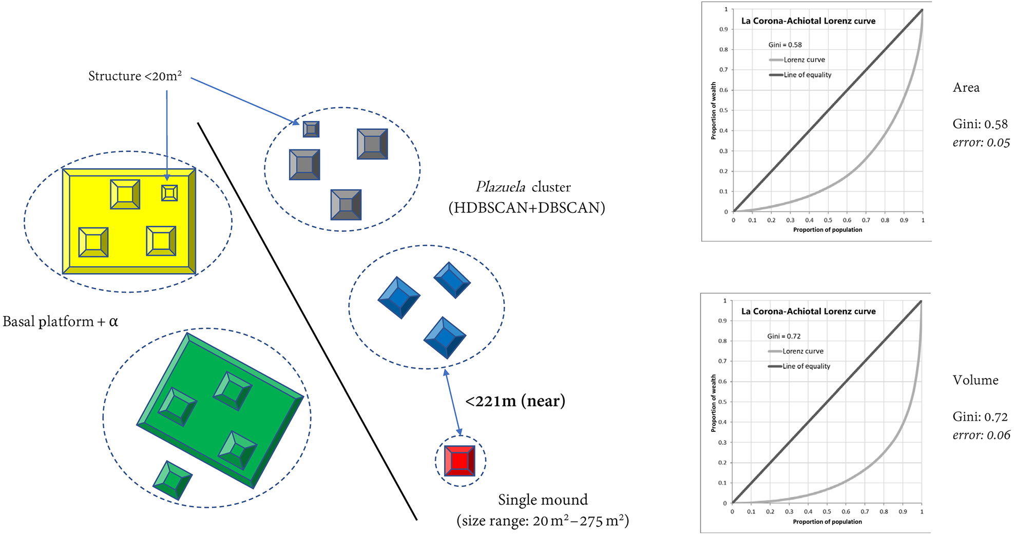
Figure 6. Gini coefficient: plazuela group, including basal platform and nearby single structures (sample size: 1,319; Scenario 4).
Results
These results suggest that the La Corona region had relatively high levels of inequality as measured by the Gini coefficient. However, one note of caution is warranted. Our Gini indices vary notably, from a low of 0.34 for area (equivalent to Canada) to a high of 0.72 for volume (higher than all modern nation states, including South Africa), solely as a function of how we aggregated our data. This variation is no small matter, since we cannot simply favor one measure without good reason.
We begin with the differences produced by area- and volume-based measurements. These are significant (see Table 1; see Thompson et al. Reference Thompson, Chase and Feinman2023). We find that volumes may be far more inaccurately measured than areas, especially given uncertainties (vertical error, misclassified points, etc.) in the LiDAR-derived DEM and further uncertainties introduced by the estimation of a pre-architectural, “natural” surface beneath digitized buildings (see Hutson et al. Reference Hutson, Stanton and Ardren2023; Munson et al. Reference Munson, Scholnick, Mejía Ramón and Paiz Aragon2023). However, because volume provides a critical dimension of information that cannot be ignored, we are not willing to discard it entirely. For this reason, we suggest calculating both area and volume, and then reporting a Gini coefficient range (see Oka et al. Reference Oka, Ames, Chesson, Kuijt, Kusimba, Gogte, Dandekar, Kohler and Smith2018, for alternative approaches to developing composite coefficients). A second source of significant Gini coefficient variation is the aggregation of different features. Thus, to choose among our four scenarios, we suggest that the one which produced the tightest range between area and volume indices is likely to be the most robust. In our case, Scenario 4—the measurement of the entire plazuela group, including nearby single mounds—results in the smallest range of values between area and volume. For this reason, we suggest that the most accurate measurement of inequality in the Corona region would be a Gini coefficient of 0.65 +/−0.06 (Table 1).
Given that our region is likely composed of two different settlement systems—a Late Classic one around La Corona to the west and a Late Preclassic one around Achiotal in the east—we divided our data to calculate separate Gini indices for these two times and sites (Table 2; see Montgomery and Moyes Reference Montgomery and Moyes2023; Shaw-Müller and Walden Reference Shaw-Müller and Walden2023). For the Late Classic La Corona polity, using our preferred measure, we see an overall Gini coefficient of 0.6 +/−0.09 (Figure 7). Frankly, we were surprised by this high value, given the secondary, satellite, or, more simply, modest nature of the site and its settlement. To drill down a bit further, we decided to isolate the settlement within two settlement clusters in order to determine the extent to which this degree of inequality varied within separate sectors of the same polity (see Marken Reference Marken2023).
Table 2. Gini coefficients of four different data subsets.
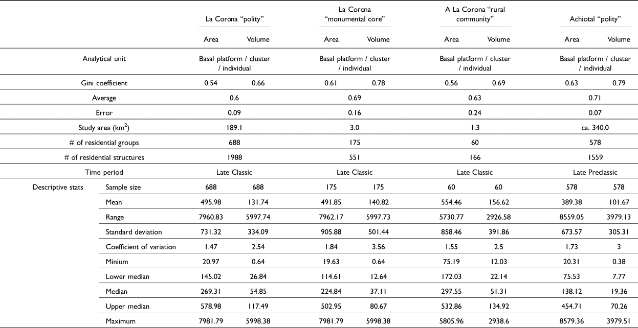
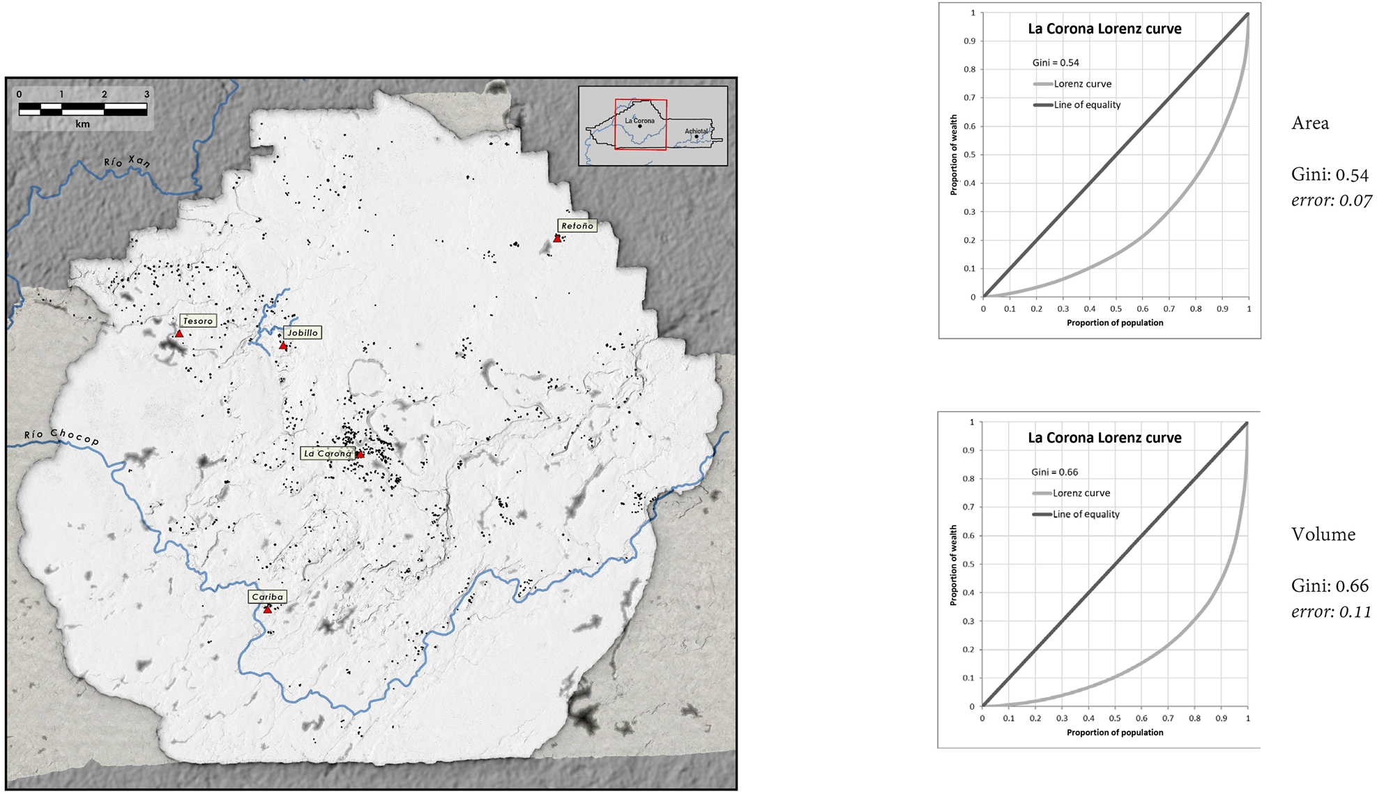
Figure 7. La Corona polity: plazuela group and nearby single structures (sample size: 688), Gini coefficient.
We first isolated the polity core (ancient Sak Nikte') and found a Gini coefficient of 0.69 +/−0.16—a value likely higher than the polity average. We then chose the largest cluster of “rural settlement” and calculated a Gini coefficient of 0.63 +/−0.24. While lower than the polity core, this value had such a wide margin of error that it is difficult to conclude anything with certainty. It nevertheless seems plausible this “rural cluster” and other smaller ones would likely demonstrate progressively less inequality. The basic takeaway here is that there was no place in the Corona polity where inequality would be sensed and perceived more acutely than in the polity core. This makes sense, as the most conspicuous architectural feature of the entire region is the La Corona palace: a huge residence in the middle of the polity core.
Surprisingly, however, these values are eclipsed by our results in the Achiotal sector of our dataset, where the settlement is predominantly Late Preclassic. Of 43 stratigraphically tested buildings in the region, all but three (93 percent) produced evidence of Late Preclassic occupation. This region produced a Gini coefficient of 0.71 +/−0.07 (Figure 8). This striking level of inequality is primarily down to a single complex: the palace at Achiotal, which dwarfs any other residential architecture in the region. To go by architecture and all the resources it indexes, it seems that the Late Preclassic was every bit as “unequal” as the Classic period in this region—indeed, likely more so.
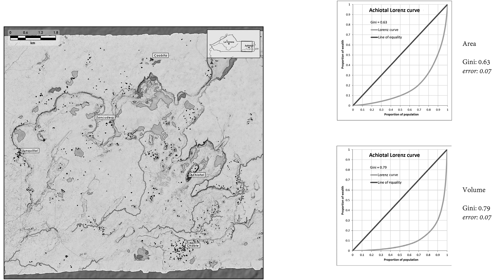
Figure 8. Achiotal polity: plazuela group and nearby single structures (sample size: 578), Gini coefficient.
To further nuance this comparison, we compared the median residential sizes of both the La Corona and Achiotal polities. The data (see Table 2) demonstrate that the median residence in the La Corona polity (269.31 m2/54.58 m3) was two to three times larger than that of the Achiotal polity (138.12 m2/19.36 m3). Although the Achiotal polity exhibits a somewhat higher degree of inequality, this difference does not fully explain the disparity in median residential size. Consequently, we propose that the disparity also suggests that Late Classic households were both sociologically larger and more complex, as well as materially wealthier, than their Late Preclassic counterparts. Whether this difference holds true across the entire Maya Lowlands will depend on the analysis of a much larger dataset.
Conclusions
Our initial foray into these analyses provides some simple takeaways that we hope will inform our continued application of this index in our efforts. First, we suggest that isolated buildings have a small, but still important effect on Gini calculation, and we need a unified strategy for dealing with these buildings. Moreover, given their ephemeral nature, we must ensure that their inclusion is buttressed by robust field verification efforts to reduce the possibility of including false positives or ignoring false negatives.
We also conclude that the La Corona region has high levels of economic inequality, particularly when the palace—a residence—is not arbitrarily excluded. In contrast, the Gini for the Late Preclassic settlement around El Achiotal is even higher than for Late Classic La Corona. This suggests that for this region, inequality did not grow with time, even though overall material wealth and household complexity apparently did. We suggest the possibility that the common factor between the extreme Gini indices for La Corona and Achiotal is that they were both “frontier” polities in their respective heydays, each dependent to some degree on relations with a foreign hegemonic power. We suspect that these values reflect the juxtaposition of a rural subsistence farming population, with essentially intrusive elite classes drawn to the region for its strategic importance. We maintain that this inequality was an expression of socioeconomic disarticulation throughout the region. In other words, this inequality may have been “felt” differently by the populations in the two areas, given the sharp divergence in overall sociopolitical complexity and differences in the relationship between ruling houses and political subjects.
Furthermore, this comparison between La Corona and Achiotal demonstrates how we should expand our analyses beyond the level of “the polity,” however we choose to define it. Although our example does not compare two contemporaneous polities, it is important to appreciate that ancient Maya people would not have assessed inequality or prosperity only at the level of an individual kingdom, but could also have compared a place like Tikal or Caracol to a place like La Corona. To put it prosaically, would the richest family at La Corona have been able to afford Tikal? It is therefore instructive for us to aggregate data—perhaps by region—so that these interregional differences can be identified and interpreted; and that the further we extend our comparisons, the more likely our values will reflect an ancient reality.
These last points bring us to our final thought. While this coefficient may bring some empirical order to our observations regarding architectural differentiation within an area, we caution against the accepting prima facie notion of “inequality” (see Munson and Scholnick Reference Munson and Scholnick2022). We cannot assume how any of these degrees of inequality were salient, if at all, to the ancient Maya. In fact, was “inequality” even a phenomenon of degree or was it seen only in absolutist terms? Perhaps inequality was understood only as a function of a “moral order” (e.g., Houston et al. Reference Houston, Escobedo, Child, Golden, Muñoz and Smith2003)? We should proceed cautiously when leveraging our understanding of these inequality indices to develop economic or sociopolitical models that inevitably touch upon indigenous notions of freedom, indebtedness, prosperity, and power.
Acknowledgements
The authors would like to thank the Fundación Patrimonio Cultural y Natural Maya-Pacunam for planning, funding, and managing the Pacunam LiDAR Initiative (PLI) that provided the LiDAR necessary for this study. We also acknowledge the NSF National Center for Airborne Laser Mapping (NCALM) at the University of Houston for the collection and processing of the 2016 LiDAR dataset. We are grateful to the Government of Guatemala's Instituto de Antropología e Historia for granting permissions, not only for the LiDAR survey, but also for PRALC to conduct the archaeological fieldwork discussed in this article.
Competing interests declaration
The authors declare they have no known competing financial interests or personal relationships that could have appeared to influence the work reported in this article.
Data availability statement
Data will be made available on request to the authors.
Funding statement
This research was made possible by funding from Fundación Patrimonio Cultural y Natural Maya-Pacunam, through contributions from the Hitz Foundation and Pacunam's Guatemalan members (Cervecería Centro Americana, Grupo Campollo, Cementos Progreso, Blue Oil, Asociación de Azucareros de Guatemala-Asazgua, Grupo Occidente, Banco Industrial, Walmart Guatemala, Citi, Samsung, Disagro, Cofiño Stahl, Claro, CEG, AgroAmerica, Fundación Tigo, and Fundación Pantaleón), the Alphawood Foundation, the Hitz Foundation, the National Geographic Society (9710-15 to Auld-Thomas), and the Middle American Research Institute at Tulane University.


 Open access