


Nomenclature
- BPF
Blade Passing Frequency
Symbols
- ${c_a}$
axial flow speed in m/s
-
${c_p}$
specific heat constant in J/ (kg K)
- n
total number of data points
-
${p_i}$
ith level division as percentage of total interval
- q i
total number of points in ith interval
- s
step size
-
$split$
splitting step size as percentage of total interval
- w
window size
- x i
time series variable
-
$H$
entropy function
- I I
ith level division of total interval
- P ref
reference pressure taken as atmospheric pressure of 101,325 Pa
-
$\Delta {T_0}$
total temperature difference in K
-
$U$
blade tip speed in m/s
- X
set of all-time series data points
- X s
set of subsets of X
- φ
flow coefficient
- ψ
loading coefficient


1.0 Introduction
Predicting stall before it occurs is crucial for avoiding stalling of a compressor/fan. Stalling can cause loss of efficiency, vibrations or even structural failure, depending on the severity of the phenomenon. Though the phenomena of stall in conventional compressors and fans have been widely investigated, the stall inception mechanisms in contra-rotating fans have not been explored thoroughly.
Stall inception in a fan/compressor remains an interesting topic of research and the works on stall inception started when Emmons [Reference Emmons, Kronauer and Rockett1] suggested a conceptual model for the rotating stall phenomenon. The research on stall inception for the next several decades focused on developing theoretical models [Reference Day, Greitzer and Cumpsty2]–[Reference Moore and Greitzer5]. Later with larger experimental studies, researchers identified the significant fluid phenomenon leading to stall and termed those as the short-length-scale spikes and the long-length-scale modal disturbances [Reference McDougall, Cumpsty and Hynes6]–[Reference Camp and Day8]. The prominent aspects of the behaviour of these fluid structures remain unclear and the research on identifying the structure and propagation of these structures are still being carried out experimentally and computationally [Reference Yamada, Kikuta, Iwakiri, Furukawa and Gunjishima9]–[Reference Brandstetter, Paoletti and Ottavy17]. Several of these works concluded the existence of the disturbances prior to the fully developed stall. With this understanding, some researchers tried to predict and control the stall phenomenon using active or passive techniques. Spakovszky et al. [Reference Spakovszky, Weigl, Paduano, Van Schalkwyk, Suder and Bright18] used an active technique using jet injectors upstream of the rotor leading edge. Control strategies were obtained using transfer functions determined from the response of the sensors. A review of the different types of stall inception phenomenon and the possible control strategies were detailed by Tan et al. [Reference Tan, Day, Morris and Wadia19]. Ashrafi et al. [Reference Ashrafi, Michaud and Vo20] used a plasma actuator placed upstream of the rotor leading edge and impeller leading edge of an axial compressor and a centrifugal compressor, respectively, to delay the stall. The plasma actuator could accelerate the flow and push the tip leakage flow into the blade passage. Recently, Day [Reference Day21] reported that even after a long history of research on stall prediction in compressors/fans, designing a stall-resistant machine or to predict the stall of a new compressor is still a challenge. Thus, it is evident that the prediction of stall needs to be investigated in detail to design a compressor/fan that is tolerant to stall or can operate over a wide range of mass flows.
Some recent studies have focused on machine learning strategies to predict the unsteady variation in pressure fluctuations to identify stall. Xu et al. [Reference Xu, Wang, Liu and Liu22] implemented a support vector regression machine (SVRM) to predict internal pressure in a fan, and detect the inception of rotating stall. The results predicted by the SVRM model are compared to the stall detected using wavelet transform of pressure data. The model successfully predicts pressure 0.0625 seconds, which corresponds to 1.35 rotor revolutions in advance and can reliably detect stall before it occurs, giving ample time for a control system to prevent it. Kim et al. [Reference Kim, Pullan, Hall, Grewe, Wilson and Gunn23] studied the stall inception behaviour of two different transonic fans both experimentally and computationally using steady and unsteady simulations. The unsteady pressure reading upstream of the leading edge of rotor is compared to the pressure traces predicted using unsteady computations and used to detect the stall and its propagation in the machine. Using CFD, the stall mechanisms of the two fans were studied, indicating tip leakage flow and shock boundary layer interaction as the cause of the stall. Unsteady casing pressure measurements at the rotor and stator of a four-stage axial compressor were used to identify and study the stall and pre-stall behaviour of compressor, at different rotor speeds by Methling et al. [Reference Methling, Stoff and Grauer24]. The stall was identified to be associated with spike-type disturbances. A neural network was trained using the pressure data at different speeds to identify the region of operation of the compressor, indicating if the machine is near stall. This network model works for both spike type stall and modal wave, at different rotor speeds if trained with sufficient data. The physics of the pre-stall instability described by discrete flow disturbances, or rotating instability was studied by Eck et al. [Reference Eck, Geist and Peitsch25], using complementary experimental and numerical methods. The instability is characterised by the development of vortex tubes that are attached to the casing and suction surface of the rotor blades. Also, a new stall indicator was developed by applying statistical methods on the casing pressure trace, to get better control of the safety margin. A K-means clustering and Gaussian Mixture Models-based algorithm was developed by Yusoff et al. [Reference Yusoff, Ooi, Lim and Leong26], using the pressure, temperature and vibration signals from LM 2500 axial compressor. The model monitors the machine condition and could avoid any fatal failure. The model also identified three machine states characteristic—off, active and abnormal—along with degradation tracking visualisation of the machine. It will be helpful in predictive maintenance of the machine. Falzone et al. [Reference Falzone and Kolodziej27] recorded vibration signals from Dresser-Rand ESH-1 reciprocating compressor, taken using accelerometers in normal and damaged condition, and these signals were used to develop a model to monitor the compressor condition. Wavelet transforms were used to identify and visualise the vibration features from the data. The first and second order wavelet statistical features were selected for training a support vector machine to classify if the machine is normal or damaged, which worked with predictive accuracy of more than 90%. It will be helpful in predictive maintenance of the machine.
From a thorough literature review, it is understood that the stall inception is still a phenomenon which requires detailed understanding and the prediction of stall can help in recovering the machine from failure. Also, most of the works that are reported in literature related to application of machine learning on compressors or fans are focused on predictive maintenance of terrestrial gas turbines, or prediction of stall for terrestrial gas turbine compressors using measurement and prediction of absolute values of various physical parameters. In this work we take a different approach based on data engineering to predict as well as detect stall in a contra-rotating fan, which is a potential configuration that can replace the conventional fans in future aircraft gas turbine engines. The methodology records casing pressure traces using high-response sensors and studies the variation in the Fourier amplitude and frequency characteristic of pressure traces as the contra-rotating fan approaches stall. Assumption is that the variation in flow characteristics in the fan as it approaches stall will be translated to casing pressure traces and its Fourier characteristic as well, which was observed in cases of compressors as reported in literature. The different regions of operation were algorithmically characterised and classified using abstract parameters and machine learning methods. Neural network models were trained to identify the operating region of the machine based on the recorded pressure traces. Control systems using these models could be made, which can detect the operating region of the machine and take necessary action to avoid stall or pull the machine out of stall. This work extends the application of machine learning to the operation of contra-rotating fans, and thus explores the potential use of machine learning for aerospace gas turbine applications. The identified flow regimes are not based on absolute value of a physical parameter, rather on the statistical features of the data, and so are related to the properties of the flow over an extended period of time. This makes the classification model resilient to noise in actual value of the physical parameter. The control model based on the above methodology has potential to significantly reduce the instrumentation for measurement and computation as it uses only one sensor to measure the pressure traces, and no other parameter is required to be measured. This work also allows gaining some insight into the stall inception characteristics of a contra-rotating fan, which has not been explored as thoroughly as in conventional rotor-stator configurations. Though the current work is focused on a specific design speed of the contra-rotating fan, the methodology presented in this work is general and can be extended to other speeds. In addition, this method being generic can also be applied to other types of machines to identify their operating flow regimes and can be used to train classification models for their control.
2.0 Methodology
2.1 Experimental setup
The experiments for this work were performed on a contra-rotating fan setup shown in Fig. 1. The contra-rotating fan has nine blades on rotor-1 and seven blades on rotor-2. The stage has a target stage loading of 1.05 at a flow coefficient of 0.79, as defined in Equations (1) and (2) respectively, and the Reynolds number obtained based on the axial velocity at the inlet and the chord of the blade is approximately 2 $ \times $
105. The important specifications of rotor1 and rotor2 is given in Table 1, and a detailed description of the design of the contra-rotating stage can be found in Manas and Pradeep [Reference Manas and Pradeep28].
$ \times $
105. The important specifications of rotor1 and rotor2 is given in Table 1, and a detailed description of the design of the contra-rotating stage can be found in Manas and Pradeep [Reference Manas and Pradeep28].
 \begin{align}\psi = \frac{{{c_p}\Delta {T_0}}}{{0.5\;{U^2}}}\end{align}
 \begin{align}\varphi = \frac{{{c_a}}}{U}\end{align}

Figure 1. Photograph of the experimental facility.
2.2 Data acquisition
Seven high response pressure sensors arranged circumferentially and equally spaced on the casing, near the leading edge of the first rotor, were used to take pressure data at 10,000Hz sampling frequency, or normalised sampling frequency of 200, with respect to the rotor frequency. The data was recorded for 30 seconds or 1,500 rotor revolutions, generating 300,000 data points during the stall inception process. A schematic of the positional arrangement of the sensors is shown in Fig. 2. In this period of 30 seconds, the machine was pushed towards the stall region from the safe operating region, by continuously reducing the mass flow rate using a throttle controller. Similar measurements were taken four times on different days, in order to verify the consistency of the data and to validate the analysis. Thus, in total, five datasets were analysed, and the validity and repeatability of the model are tested. The data from the first experiment is referred to as the Baseline case in the paper and the other four are referred to as Test cases. All sensors showed similar trends for a given experiment, and therefore, for further analysis, data from only one sensor is used.

Figure 2. Schematic of the sensor position.
2.3 Analysis methodology
In order to understand the characteristics of the pressure data, two methodologies are used in this study. One is the windowed Fourier, and the other is the identification of the abstract statistical parameters that can help to divide the pressure traces into different operating regions. The algorithms of both the methods are described here.
2.3.1 Windowed fourier analysis
Windowed Fourier analysis is similar to short-time Fourier analysis, but without using the hamming functions. Let ‘X’ be a set of ‘n’ time series data points, X = {x 1, x 2,…, x n }. Let ‘w’ be the window size and ‘s’ be the step size such that the points are divided into subset of X given by, X s = [{x 1, x 2,…, x w }, {x 1+s, x 2+s ,…., x w+s }, …, {x 1+ks, x 2+ks,…, x w+ks}]. Here, the sets are mutually exclusive if ‘s ≥ w’, else, the sets have an overlap of ‘w - s’ points and also, ‘w + ks ≤ n’. The window and step sizes affect the details of the information that can be extracted from the data. The discrete Fourier transform for each of the set in Xs is performed, and the index set for each of the set is defined as I = [{mean (1, 2,…, w)}, {mean (1+s, 2+s,…, w+s)},…, {mean (1+ks, 2+ks,…, w+ks)}]. The Fourier frequency vs Fourier amplitude vs index is plotted to get an insight into how the amplitude of various frequencies vary with the index.
Table 1. Specifications of rotor-1 and rotor-2

For the time series data used in this work, the number of data points, n = 300,000. Window size, w = 1,000 and step size, s = 100 were chosen after a few iterations with different values. The chosen values ensure that both frequency and temporal resolutions are satisfactorily achieved, and one is not overly compromised for the other. The current choice of window size corresponds to five rotor revolutions and the step size corresponds to 0.5 rotor revolutions. The step size should be small enough to accurately capture the development of the stall in time, and window size should be large enough to capture sufficient data points for resolving the frequencies and establish the flow regime in which the machine is operating. If the flow characteristics of the machine did not change for multiple rotations, it can be established with some confidence that the machine is operating in that flow regime. It was observed that if the size of the window is increased, the parameters computed using the Fourier amplitudes get smoothed out, and the resolution of the features in time reduces. This can cause issues near the stall region as it will limit the accuracy of the algorithm to exactly determine the time at which stall starts. Therefore, too much compromise on time resolution will not be good to capture the start point of the stall. Also, if the time resolution is significantly reduced, the frequency content of the window is not appropriately resolved. This further leads to an increase in the number of windows and thus the computational time, which was found to be not necessary for the present analysis. As far as the step size is concerned, a larger step size reduces time resolution of computed features and a smaller step size increases computational time. However, the above choice of window size and step size could be formalised based on the fact that the current window size of 1,000 points is equivalent to five rotor revolutions, and a step size of 100 points is equivalent to 0.5 rotor revolutions. It was found that the significant pre-stall disturbances and the stall cells during the fully developed stall travel approximately at 0.5 times the blade speed. Therefore, the choice of 0.5 rotor revolutions allows to appropriately capture the movement of pre-stall disturbances and the stall cell. Also, sufficient data points are required to resolve the frequencies. Here, the sampling frequency of the sensors is 10kHz. Therefore, five rotor revolutions at a given RPM were required to capture 1,000 data points. And the value of pressure must be recorded across multiple rotations for the present methodology to be applicable as it predicts the operating regime based on flow dynamics, and consistent flow dynamics across multiple rotations confirm that the machine is operating in the predicted region. Thus, the choice of the window size is a function of the machine RPM, sensor sampling frequency, minimum number of rotations required to capture sufficient data points to accurately capture the frequencies and the operating regime of the machine with confidence, and to resolve the time at which stall starts as accurately as possible. For step size, in addition to the above parameters, the number of rotations required for stall cells to fully develop is an important factor. The algorithm for this approach was implemented using Python 3.6.
2.3.2 Statistical parameters
The next step was to quantify the data using statistical and abstract quantities. Statistical quantities such as variance, skewness, and kurtosis for the data and Fourier amplitude of the data were initially explored, in order to quantitatively characterise the three different regions identified from the previous analysis. Later, abstract quantities like Shannon’s entropy based on two different probability definitions, for both the data and Fourier amplitude, and the coefficient of determination for a polynomial fit of a fixed degree, were also explored for the same. Finally, four quantities were chosen for this purpose, which are the variance of Fourier amplitude, two different Shannon’s entropies, and the coefficient of determination for a polynomial fit of fixed degree. Two different algorithms for calculating Shannon’s entropy for a given data, as used in this work are described below.
Consider a set X = {x 1, x 2,…, x n }. First, the elements of the set X are transformed as
 \begin{align}{x_i} \to \;{x_i}/\Sigma {x_i}\end{align}
Here, all elements lie in the range $0 \le {x_i} \le 1$
, and their sum adds up to one, making it a probability like mapping on the data.
$0 \le {x_i} \le 1$
, and their sum adds up to one, making it a probability like mapping on the data.
Now, Shannon’s entropy 1 is calculated as
 \begin{align}H = - \Sigma {x_i}{\rm{ln}}\;{x_i}\end{align}
Consider a set X = {x 1, x 2,…, x n}. The range min(X) and max(X) is divided into uniformly spaced intervals where the element of the interval set is given by
 \begin{align}{I_i} = \;{\rm{min}}\left( X \right) + \left\{ {{\rm{max}}\left( X \right) - {\rm{min}}\left( X \right)} \right\}\left( {\frac{{{p_i}}}{{100}}} \right)\end{align}
where ${p_0} = 0$
and
${p_0} = 0$
and ${p_i} = \;{p_{i - 1}} + split$
. Here,
${p_i} = \;{p_{i - 1}} + split$
. Here, $split$
is defined as the interval spacing or the difference between two intervals in percentage of the total interval
$split$
is defined as the interval spacing or the difference between two intervals in percentage of the total interval $\;{\rm{max}}\left( X \right) - {\rm{min}}\left( X \right)$
. For each interval {
$\;{\rm{max}}\left( X \right) - {\rm{min}}\left( X \right)$
. For each interval { ${I_i}$
,
${I_i}$
, ${I_{i + 1}}$
}
${I_{i + 1}}$
}
 \begin{align} q_{i} = size [\{x_{p}\;:\; l_{i} \leq x_{p} \leq l_{i+1};\; x_{p} \epsilon X \}] \end{align}
is calculated. Thus, Shannon’s entropy 2 is calculated as
 \begin{align}H = - \Sigma \left( {\frac{{{q_i}}}{{size\left( X \right)}}} \right){\rm{ln}}\;({q_i}/size\left( X \right))\;\end{align}
where $\;{q_i} \gt 0$
and
$\;{q_i} \gt 0$
and $\dfrac{{{q_i}}}{{size\left( X \right)}}$
acts as probability-like mapping on the data.
$\dfrac{{{q_i}}}{{size\left( X \right)}}$
acts as probability-like mapping on the data.
The idea behind these algorithms is to fit a probability distribution on a given data set, so that each point in the data can be assigned a value between 0 and 1, in order to calculate the entropy values. There is no physical meaning of these probability-like distributions in relation to the actual data. If the same probability distribution function is applied to two different data sets having a different distribution, the probability assigned to the data points will differ and will be reflected in the value of Shannon’s entropy. A different distribution will generate a different entropy value. Similarly, a different probability distribution on the same data will generate a different entropy value.
If the physics of the flow in a different operational region is different, then the distribution of pressure and the Fourier amplitude data in that region will be different. If the same probability distribution function is applied in each of these regions, they will generate different entropy values and different regions can be identified using these values.
The two entropy values and the goodness of fit were calculated for each window and plotted with respect to the index. The window and index were the same as used in the Fourier analysis. The value of split was chosen to be 0.02% for evaluating Shannon’s entropy 2, so that the distribution of data points with respect to amplitude was captured with highest resolution while staying within a small computational time limit of a few 100 milliseconds, and also resolve the different flow regimes. A polynomial of degree 50 was chosen for evaluating the goodness of fit. The choice of degree 50 was based on an analysis, which identified that in the flow regime showing periodic disturbances, the coefficient of determination was proportionally related to the degree of polynomial, and in regions where there was no periodic disturbance, no correlation was found. Since the number of data points were large, a polynomial of higher degree was more likely to accurately model it. Therefore, a higher-degree polynomial could resolve different flow regimes and the upper limit of the choice of the degree of polynomial was set based on the computational time.
Since the data was unmarked, the unsupervised learning algorithm, K-means clustering, was applied on these four quantities to classify the data into different groups. It clearly identified three clusters with large and stable silhouette values for all five tests, marking the three different regions in the original time series. This marked data was used to train neural network classifiers and could successfully predict the operating region of the machine with acceptable accuracy.
3.0 Results and discussion
3.1 Fourier analysis of pressure data
Preliminary Fourier analysis was performed on pressure data from all seven sensors, from all five experiments, for full 300,000 data points, taken at normalised sampling frequency of 200, giving a normalised Nyquist frequency of 100. All seven sensors showed a similar trend in the frequency vs amplitude plots as shown in Fig. 3. Most of the significant normalised frequencies are in the range 0–9, which is below the first blade passing frequency, as marked by red ellipse. It can also be observed that the amplitude is decreasing rapidly for larger frequencies.

Figure 3. Fast Fourier transform of the pressure data of one sensor.
Figure 4 shows the windowed Fourier analysis performed on the data to understand the variation of frequency and amplitude. The amplitudes have been filtered so that all frequencies with amplitude above 0.987 and below 0.0691 are set to 0, in order to highlight the distinction between the three regions. It can be observed that none of the Fourier frequencies has any significant amplitude prior to approximately 500 rotor revolutions (marked by the red line). Some frequency excitations are observed between 500 rotor revolutions and around 950 rotor revolutions (marked by the green line). The excitations are intermittent and there is no order in which the frequencies are excited, except that most of the excited frequencies are below the first blade passing normalised frequency corresponding to 9. Also, the amplitudes of excitation for various frequencies increase as the rotor moves from 500 to 950 revolutions or towards stall. This region identified before the fully developed stall is the transition region. Beyond 950 rotor revolutions (green line), the stage enters into a fully developed stall. Moreover, it can be observed that the larger frequencies (beyond the first blade passing frequency) also get excited as the machine moves towards stall, with smaller frequencies having larger amplitudes.

Figure 4. Frequency vs number of rotor revolutions vs amplitude (colour bar).
From Fig. 5, it can be concluded that the stall region is characterised by the consistent frequency excitation through the region at a regular interval of approximately 0.6, which marks the harmonics of the stall cell normalised frequency. Yellow line marks the first blade passing normalised frequency at 9. By observing the region enclosed by the blue square in Fig. 5, the intermittent and random excitation of frequencies that are visible in the transition region is also visible in the stall region. Another noticeable feature observed between a normalised frequency range of 4.8 and 7.2 is that the amplitude of the harmonics of stall cell frequency has dropped significantly, compared to the harmonics below 4.8 and above 7.2, and is in the same amplitude range as the intermittent random frequency excitations. It can be concluded that in the fully developed stall region, the stall cell frequency has been superimposed over the disordered frequency excitations of the transition region. The stall cell frequency marks the difference in the transition and stall regions.

Figure 5. Frequency vs number of rotor revolutions vs amplitude (colour bar) for normalised frequency range of 0–9.
Figure 6 is a different representation of Fig. 4 and highlights the amplitude range of the higher frequencies, as all the frequencies having amplitude above 0.02961 have been filtered and set to zero. Before 500 rotor revolutions, most of the frequencies have smaller amplitudes, which started rising as the rotor moved to the transition region and towards fully developed stall. A general trend marked by the orange curve shows the increasing excitation amplitude of higher frequencies as the rotor moves towards fully developed stall. It can be concluded that the high-frequency disturbances are generated in the flow as stall is approached, by some mechanism that has not been explored in detail in this work.

Figure 6. Frequency vs number of rotor revolutions vs amplitude (colour bar). Frequencies with amplitude above 0.02961 are filtered.
3.2 Characterisation of flow regimes using abstract parameters
Most of the large amplitude disturbances have normalised frequencies below 8 in both transition and the fully developed stall region as can be observed from Fig. 4 and also the three regions show significant differences in their frequency–amplitude characteristics. This indicates that the distribution of amplitude in the frequency as well as time domain is different for the three regions. This difference should be sufficient to distinctly characterise the three regions using abstract mathematical parameters, which take advantage of the above stated fact.
Many statistical and abstract parameters like variance, variance of Fourier amplitude, skewness, kurtosis, Shannon’s entropy and coefficient of determination were plotted for the data with the same window and step size as used in the windowed Fourier analysis, but only for the normalised frequency range of 1–8, filtered using Butterworth band-pass filter of order 5. Of all the parameters, four parameters were selected as they showed significantly distinct trends in the three regions of operation compared to all other parameters. Hence, these parameters are able to distinguish the regions independently. These four parameters are variance of Fourier amplitude, coefficient of determination for polynomial fit of fixed degree on the pressure data, Shannon’s entropy using the first algorithm for Fourier amplitude where all amplitude below 0.0987 and above 0.987 is set to 1 so that they contribute negligibly to the value of entropy compared to amplitudes in the required range, and Shannon’s entropy using second algorithm for the pressure data.
Figures 7–10 shows the plot of the four different parameters vs number of rotor revolutions for the baseline case. The respective magnitudes of each of these parameters are approximately in the same range for all the five experiments. All five experiments show similar trends in the variation of these parameters as shown from Figs 11–14. In case of the variance of Fourier amplitudes, initially the value is small and uniform, and then some small peaks start to develop intermittently, as expected (see Fig. 5), signifying the transition region, and later a sudden jump in the value occurs with a large peak, marking the beginning of the stall region. A similar trend is observed in the other parameters also. In the case of Shannon’s entropy 1, initially the value is small with a general straight-line trend, and then some small peaks start to develop intermittently with increasing magnitudes with large fluctuations, which marks the transition region. This is followed by a relatively stable region having comparatively large magnitude and low fluctuations in value, which marks the fully developed stall region. In the case of the coefficient of determination, similar to that of the variance of Fourier amplitude, the initial value is small with a general straight-line trend, and then some small peaks start to develop intermittently with increasing magnitude as the machine moves towards stall, marking the transition region and followed by a sudden jump in the magnitude of the variable, generating a large peak, marking the start of the fully developed stall region. For Shannon’s entropy 2, in the transition region, the fluctuations are large compared to the stall region. Though, the end of the transition region and the beginning of the stall region are not sharply distinguishable.

Figure 7. Variance of Fourier amplitude for the first experiment.

Figure 8. Shannon’s entropy using the first algorithm evaluated on Fourier amplitude for the first experiment. Amplitude filtered between 0.0987 and 0.987.

Figure 9. Coefficient of determination for a polynomial of degree 50, fitted to the data in each window, for the first experiment.
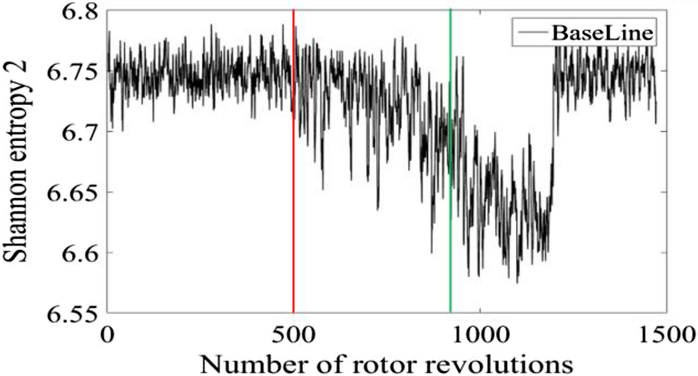
Figure 10. Shannon’s entropy using second algorithm evaluated on pressure data, for the first experiment.

Figure 11. Variance of Fourier amplitudes after min-max normalisation for each experiment.

Figure 12. Normalised Shannon’s entropy using first algorithm, for Fourier amplitudes lying between 0.987 and 0.0987 for each experiment.

Figure 13. Coefficient of determination for a polynomial of degree 50, min-max normalised for each experiment.

Figure 14. Shannon’s entropy using second algorithm min–max normalised for each experiment.
Each of these four variables show significantly distinct characteristics in the three regions identified from the windowed Fourier analysis as in Fig. 5; also, they can distinguish the three regions independently of each other. This was not necessarily true for all other variables that were tested, and hence only these four variables were selected for further analysis.
3.3 Discrete clustering of operating region using machine learning
All the four variables that were selected show distinct characteristics in the three regions identified using windowed Fourier analysis; however, these differences are not sharply identifiable in all cases and are gradual with large fluctuations. If an algorithm has to prevent stalling of the machine, it should discretely identify the three regions with high confidence, so that whenever the machine reaches the transition region, action to prevent stall could be taken.
One method to discretise is to cluster the data into distinct groups. For this purpose, K-means clustering and self-organising maps were used. However, since K means clustering was easier to implement and more transparent when dealing with the data, it was chosen for grouping the data. The average silhouette value for the clusters and the stability of average silhouette value over multiple clustering runs were used to confirm the reliability of the clustering. If in each clustering run, the average silhouette value changes, then the clustering is unreliable as each time the data points are clustered differently.
The four variables and their trends have different scales separated by multiple orders of magnitude. For example, the variance of Fourier amplitudes is seven orders of magnitude larger than all other variables. This creates a problem for clustering algorithms as it can bias the algorithm towards one of the variables. It is important to rescale all the variables into nearly the same range while preserving their trend, and min-max rescaling is one of the best ways to do it.
Data from all five experiments show similar trends and are in a similar magnitude range; however, these data do not have the exact same minimum and maximum value. Therefore, to rescale the variables, some threshold maximum and threshold minimum value should be chosen that is valid across all the five experiments. The repeatability of trend and magnitudes across all five experiments indicates a physical origin of the chosen parameters, even if they are abstract. This allows us to choose a specific threshold maximum and minimum value for each of the parameters that is valid across the experiments, to do the min-max rescaling that puts all the parameters roughly in the range of 0–1 while preserving their trends. This can be done through a direct observation of the magnitudes, or by taking the average of the maxima and minima of a given parameter over all the experiments. For this work, the thresholds were chosen by direct observation of the data plots (similar to Figs 7–10) for all five experiments. Table 2 gives the different parameters and their chosen min-max threshold values.
All the four parameters were rescaled using the corresponding min-max threshold values, and then K-means clustering algorithm was applied to these parameters with 2, 3, 4 and 5 clusters. Figure 15 shows the variation of silhouette value with the number of iterations for the baseline case. It can be concluded that cluster 1, where the data is separated into two clusters, has an almost stable silhouette value of 0.874308 with very small fluctuations, and cluster 2, where the data is separated into three clusters, has a perfectly stable silhouette value of 0.855883, across all the iterations of the algorithm. Cluster 3 that divides the data into four clusters, and cluster 4 that divides the data into five clusters, are having unstable and relatively lower silhouette values. It can be concluded that the best and reliable way to cluster the given data is in two or three different groups.

Figure 15. Silhouette value vs iteration plot for different number of clusters for the baseline case.
Figure 16 shows the discrete division of clusters with rotor revolutions for two clusters (a) and three clusters (b). The red and green lines on both the figures approximately divide the three regions as identified in Fig. 5. It can be seen that, for two clusters, the transition region (between the red and green lines) shows an intermittent development of second cluster and a stable second cluster in the stall region (beyond the green line). For three clusters, the transition region shows intermittent development of second cluster and a stable third cluster in the stall region. Also, the beginning and end of each region as predicted by clustering using three clusters matches approximately with the one identified using direct observation from the windowed Fourier analysis (Fig. 5). Also, the transition region shows an intermittent development of the second cluster, which is similar to the intermittent excitation of Fourier frequencies in the transition region as observed using Fourier analysis. It can be said that before the occurrence of a fully developed stall, the machine gives intermittent pre-stall signals, and this region of operation can be called the transition region, which falls between the region of safe operation and the region of fully developed stall. The above trend was observed in all five experiments. Table 3 gives the silhouette value for two and three clusters for all the five experiments. All these values are stable across multiple iterations.

Figure 16. Discrete division of clusters with rotor revolution for (a) two clusters and (b) three clusters.
Table 2. Statistical parameters and their threshold minimum and maximum values

Table 3. Silhouette value for two and three clusters for all the five experiments

Thus, K-means clustering on the selected abstract parameters allowed discrete division and identification of the three regions, which also confirms the observation made using windowed Fourier analysis, enabling the development of an algorithm for control system that can identify the transition region using pre-stall signals, so that stall can be avoided.
3.4 Neural network based classifier for identifying operating region of the machine
K-mean clustering showed that the data can be reliably classified into three distinct clusters, corresponding to three different operating regions of the machine as observed from Fourier analysis. In order to prevent stall in the machine, the algorithm should be able to identify the region in which the machine is operating. For this, a neural network-based classification model was chosen, and the network was programmed using the Keras library in Python 3.6. Two different approaches were used to train a classification model. In the first approach, the model takes four parameters as input and gives an output corresponding to the cluster in which the given data point belongs. This model had four inputs and four outputs. The four inputs were the four parameters, and the four outputs correspond to the four columns of one hot encoded output corresponding to the cluster number. Cluster 1 was encoded as [0 1 0 0], cluster 2 as [0 0 1 0] and cluster 3 as [0 0 0 1]. Data from the baseline case and Test1 were stacked together, containing a total of 5,878 data points and this data was used to train the neural network. The same training data was used to test the trained network models and get the loss and accuracy value. The prediction made by the models, in hot encoded form, was integer encoded to directly get the cluster number, and was used to generate the confusion matrix. Also, the data from Test2, Test3 and Test4, containing a total 8,817 data points were stacked together and were used to test the network models, calculating the loss and accuracy. The confusion matrix was generated for the testing data as well using the same procedure as used for the training data. The structure, defining parameters and performance of the model, is given below, and also summarized in Tables 4–6.
For this model the total number of parameters was 1,864, out of which all were trainable parameters. Mean-squared error loss function was used to calculate the losses along with Adam optimisation algorithm with accuracy as evaluation metric. Model was trained for 20,000 epochs with batch size of 5,878. The accuracy and loss on the training data was 100% and 0 respectively, and the accuracy and loss on the testing data was 98.42% and 0.01 respectively.
Table 4. Network structure of first model

Table 5. Confusion matrix for training data for first model

Table 6. Confusion matrix for testing data for first model

In the second approach, a 1D convolution network model was used. It directly takes the min – max normalised 1,000 sensor data points of a particular window as input and generates the output corresponding to the cluster in which the given data belongs, and thus the model has 1,000 input points. Similar to the previous model, this model also has four outputs corresponding to one hot encoded classification vector as in the previous case. The training and testing methodology was the same as that of the previous model. The structure, defining parameters and performance of the model is given below, and is also summarized in Tables 7–9.
The number of windows with 1,000 data points in the training set was 5,878, which includes the data from the baseline and Test1. Similarly, the number of windows with 1,000 data points in the testing set was 8,817, which includes data from Test2, Test3 and Test4. Here, the total number of trainable parameters was 418,654. Mean-squared error loss function was used to calculate the losses along with Adam optimisation algorithm with accuracy as evaluation metric. The model was trained for 200 epochs with a batch size of 64. For this model, the accuracy and loss on the training data was 98.93% and 0.01 respectively, and the accuracy and loss on the testing data was 94.17% and 0.02 respectively.
Network model based on both the approaches showed acceptable accuracy in predicting the operating region of the machine based on clusters. Though the first model has more accuracy compared to the second model, the second model eliminates the need to compute the four abstract parameters and directly works with the sensor data as input. The intended application of the neural network models is in controlling the operating region of the machine during real time operation, thus preventing the machine from stalling. A simple conceptual schematic of a control loop based on the above models is shown in Fig. 17.
Table 7. Network structure of second model

Table 8. Confusion matrix for training data for second model

Table 9. Confusion matrix for testing data for second model


Figure 17. A simple control loop concept implementing classification network model for controlling the state of the machine.
Since the models were trained on a window size of 1,000 data points, the control loop shown in Fig. 17 takes the input as 1,000 pressure data points, which is worth 0.1 seconds of sensor data with sampling rate of 10,000Hz. In the first model, the four abstract parameters used for clustering are calculated and normalised using threshold normalisation values corresponding to that particular variable, determined using multiple experiments on the machine, as data pre-processing step. Normalised parameters are given as input to the trained model, which generates the output corresponding to the operating region of the machine. A state-based control model generates the necessary instructions to control the machine and prevent stall. The second model is also used in a similar way; however, it eliminates the need to compute the four abstract parameters. It directly takes the 1,000 pressure data samples as input, and in the pre-processing step it min–max normalises the sample and feeds it as input to the 1D convolution model, which predicts the operating region of the machine. The above method allows controlling the state of the machine based on the dynamics of the flow in the machine, as it depends on statistical features of the pressure traces over an extended period, rather than on the specific value of a flow variable at a given time, making the models resilient to noise in actual value of the flow variable.
4.0 Conclusion
The main objective of this work was to identify any pre-stall signal that the machine generates and to predict stall before it occurs, which can later be used to make a control system to prevent stall, using the pressure traces from the casing of a contra-rotating fan. Windowed Fourier analysis was performed on the pressure data to understand the variation in its frequency amplitude characteristic, as the machine moves towards the fully developed stall. The variation was expected as the distribution of pressure data will differ in different flow regimes due to different flow physics.
The windowed Fourier analysis showed pre-stall excitations at various frequencies. These excitations were random and intermittent with respect to frequencies and rotor revolutions. This was called the transition region. Stall region was characterised by a large and stable excitation of different frequencies that were integral multiple of the normalised stall cell frequency of approximately 0.6. Random and intermittent excitations that were observed in the transition region also appeared in the stall region with stall cell frequencies superimposed over it.
Four abstract parameters were chosen to quantitatively characterise these regions. All these parameters showed similar trends and also had similar respective magnitude range across multiple experiments, indicating a physical origin by virtue of repeatability. These parameters showed different trends in different regions of operation of the machine that were identified from previous analysis, but transition from one region to the other was not always sharply defined.
K means clustering was performed on the data that showed a stable classification and large silhouette value for two and three clusters. For three clusters, the second cluster marking the start and end of the transition region is around the same location as identified using the windowed Fourier analysis. These clusters discretely mark the three regions of operation of the machine, with the first cluster marking normal region, the second cluster marking the transition or pre stall region and the third cluster marking the stall region.
The clustered data was used to train two different neural network classifier models. The first model takes the four abstract parameters as input and gives the cluster number as output, indicating the region of operation of the machine. The second model directly takes 1,000 pressure data points that are min–max normalised and predicts the operating region. Both the models showed acceptable accuracy in predicting the operating region of the machine. If the machine is operating in the transition region, appropriate measures can be taken to prevent stalling of the machine, using the proposed control loop, based on the models.
The neural network models generated in this work are only applicable to this particular machine; however, the methodology presented in this work to generate these models is fairly general, and can be used to generate models for any machine working at any operating condition. Therefore, this novel methodology stands as a potential tool and can become a standard technique for identifying operating regions and training classification models across a wide range of similar turbomachines working at different operating conditions.


 Open access