

Extending this famous verse, we can also say that there is a time for work and a time for play. There is a time for leisure.
An important distinction, however, needs to be made between the precise concept of a time for leisure and the semantically different and much fuzzier notion of leisure time, the initial topic. In the course of exploring this subject, the fundamental economic forces that affect and motivate spending on all forms of entertainment goods and services will be revealed. The perspectives provided by this approach will enable us to see how entertainment is defined and how it fits into the larger economic picture.
1.1 Time Concepts
Leisure and Work
Philosophers and sociologists have long wrestled with the problem of defining leisure – the English word derived from the Latin licere, which means “to be permitted” or “to be free.” Leisure has, in fact, usually been described in terms of its sociological and psychological (state-of-mind) characteristics.1 And closely tied into this is the more recent notion that “play” is a fundamental aspect of life.2
The classical attitude was epitomized in the work of Aristotle, for whom the term leisure implied both availability of time and absence of the necessity of being occupied. According to Aristotle, that very absence is what leads to a life of contemplation and true happiness – yet only for an elite few, who do not have to provide for their own daily needs. Reference VeblenVeblen (1899) similarly saw leisure as a symbol of social class (and status emulation as a driver of demand). To him, however, it was associated not with a life of contemplation but with the “idle rich,” who identified themselves through its possession and its use.
Leisure has more recently been conceptualized either as a form of activity engaged in by people in their free time or, preferably, as time free from any sense of obligation or compulsion.3 The term leisure is now broadly used to characterize time not spent at work (where there is an obligation to perform).4 Naturally, in so defining leisure by what it is not, metaphysical issues remain largely unresolved. There is a question of how to categorize work-related time such as that consumed in preparation for, and in transit to and from, the workplace. And sometimes the distinctions between one person’s vocation and another’s avocation are difficult to draw: People have been known to “work” pretty hard at their hobbies.
Although such problems of definition appear quite often, they fortunately do not affect analysis of the underlying economic structures and issues.
Recreation and Entertainment
In stark contrast to the impressions of Aristotle or Veblen, today we rarely, if ever, think of leisure as contemplation or as something to be enjoyed only by the privileged. Instead, “free” time is used for doing things and going places, and the emphasis on activity corresponds more closely to the notion of recreation – refreshment of strength or spirit after toil – than to the views of the classicists.
The availability of time is, of course, a precondition for recreation, which can be taken literally as meaning re-creation of body and soul. But because active re-creation can be achieved in many different ways – by playing tennis or by going fishing, for example – it encompasses aspects of both physical and mental well-being. Hence, recreation may or may not contain significant elements of amusement and diversion or occupy the attention agreeably. For instance, amateurs training to run a marathon might arguably be involved in a form of recreation. But if so, the entertainment aspect would be rather minimal.
As noted in the Preface, however, entertainment is defined as that which produces a pleasurable and satisfying experience. The concept of entertainment is thus subordinate to that of recreation: It is more specifically defined through its direct and primarily psychological and emotional effects.
Time
Most people have some hours left over – “free time,” so to speak – after subtracting the hours and minutes needed for subsistence (mainly eating and sleeping), for work, and for related activities. But this remaining time has a cost in terms of alternative opportunities forgone.
Because time is needed to use or to consume goods and services, as well as to produce them, economists have attempted to develop theories that treat it as a commodity with varying qualitative and quantitative cost features. However, as Reference SharpSharp (1981) notes in his comprehensive book, economists have been only partially successful in this attempt:
Although time is commonly described as a scarce resource in economic literature, it is still often treated rather differently from the more familiar inputs of labor and materials and outputs of goods and services. The problems of its allocation have not yet been fully or consistently integrated into economic analysis.
Investigations into the economics of time, including those of Reference BeckerBecker (1965) and Reference DeSerpaDeSerpa (1971), have suggested that the demand for leisure is affected in a complicated way by the consumption-cost of time. For instance, according to Reference BeckerBecker (1965; see also Reference Ghez and BeckerGhez and Becker 1975):
The two determinants of the importance of forgone earnings are the amount of time used per dollar of goods and the cost per unit of time. Reading a book, getting a haircut, or commuting use more time per dollar of goods than eating dinner, frequenting a nightclub, or sending children to private summer camps. Other things being equal, forgone earnings would be more important for the former set of commodities than the latter.
The importance of forgone earnings would be determined solely by time intensity only if the cost of time were the same for all commodities. Presumably, however, it varies considerably among commodities and at different periods. For example, the cost of time is often less on weekends and in the evenings.
From this it can be seen that the cost of time and the consumption-time intensity of goods and services – e.g., commitment, is usually higher for reading a book than for reading a newspaper – are significant factors in selecting from among entertainment alternatives. “Time is what remains scarce when all else becomes abundant.”5 Time indeed is money.
Expansion of Leisure Time
Most of us are not commonly subject to sharp changes in our availability of leisure time (except on retirement or loss of job). Nevertheless, there is a fairly widespread impression that leisure time has been trending steadily higher ever since the Industrial Revolution of more than a century ago. Yet the evidence on this is mixed. Figure 1.1 shows that in the United States the largest increases in leisure time – workweek reductions – for agricultural and nonagricultural industries were achieved prior to 1940 and had already been reflected in rising interest in entertainment as early as the 1920s.6

Figure 1.1. Estimated average weekly hours for all persons employed in agricultural and nonagricultural industries, 1850–1940 (ten-year intervals) and 1941–56 (annual averages for all employed persons, including the self-employed and unpaid family workers).
But more recently, the lengths of average workweeks, adjusted for increases in holidays and vacations have scarcely changed for the manufacturing sector and have also stopped declining in the services sector (Table 1.1 and Figure 1.2). By comparison, average hours worked in other major countries, as illustrated in Figure 1.3, have declined markedly since 1970.
Table 1.1. Average weekly hours at work, 1948–2018,a and median weekly hours at work for selected years
| Year | Average hours at work | Median hours at work | ||
|---|---|---|---|---|
| Unadjusted | Adjustedb | Year | Hours | |
| 1948 | 42.7 | 41.6 | 1975 | 43.1 |
| 1956 | 43.0 | 41.8 | 1980 | 46.9 |
| 1962 | 43.1 | 41.7 | 1987 | 46.8 |
| 1969 | 43.5 | 42.0 | 1995 | 50.6 |
| 1975 | 42.2 | 40.9 | 2004 | 50.0 |
| 1986 | 42.8 | 2018 | 43.5 | |
a Nonstudent men in nonagricultural industries.
b Adjusted for growth in vacations and holidays.
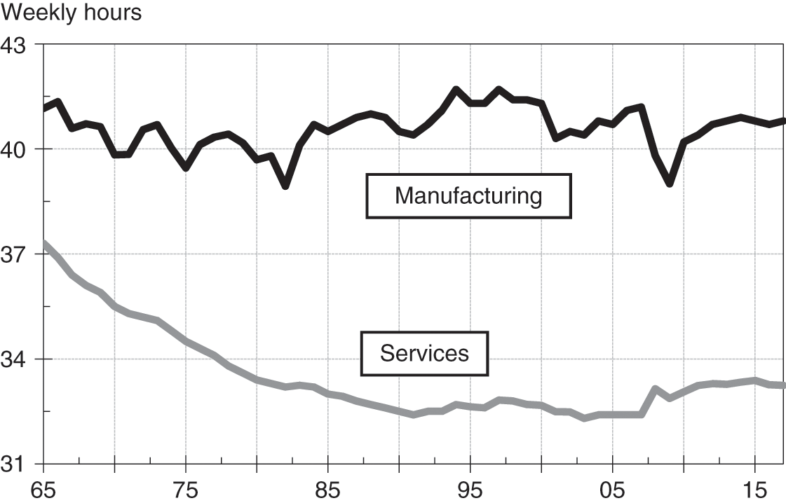
Figure 1.2. Average weekly hours worked in manufacturing and service industries 1965–2018.

Figure 1.3. Average annual hours worked by persons employed (U.K. series changed after 2010), 1970–2018.
Although this suggests that there has been little, if any, expansion of leisure time in the United States, what has apparently happened instead is that work schedules now provide greater diversity. As noted by Reference SmithSmith (1986), “A larger percentage of people worked under 35 hours or over 49 hours a week in 1985 than in 1973, yet the mean and median hours (38.4 and 40.4, respectively, in 1985) remained virtually unchanged.”7
If findings from public-opinion surveys on Americans and the arts are to be believed, the number of hours available for leisure may actually at best be holding steady.8 But occasionally the view that Americans are actually working more hours than previously has been expressed.9
Reference Aguiar and HurstAguiar and Hurst (2007) argue the opposite. And as shown in Table 1.2, Reference McGrattan and RogersonMcGrattan and Rogerson (2004) found that since World War II, the number of weekly hours of market work in the United States has remained roughly constant, even though there have been dramatic shifts in various subgroups.
Table 1.2. Aggregate weekly hours worked per person (+15), 1950–2000
| Year | Aver. weekly hours worked | Employment-to-population ratio (%) | |
|---|---|---|---|
| Per person | Per worker | ||
| 1950 | 22.34 | 42.40 | 52.69 |
| 1960 | 21.55 | 40.24 | 53.55 |
| 1970 | 21.15 | 38.83 | 54.47 |
| 1980 | 22.07 | 39.01 | 56.59 |
| 1990 | 23.86 | 39.74 | 60.04 |
| 2000 | 23.94 | 40.46 | 59.17 |
| % change: 1950–2000 | 7.18 | −4.56 | 12.30 |
Reference RobinsonRobinson (1989, p. 34) also measured free time by age categories and found that “most gains in free time have occurred between 1965 and 1975 [but] since then, the amount of free time people have has remained fairly stable.” By adjusting for age categories, the case for an increase in total leisure hours available becomes much more persuasive.10
In addition, Reference Roberts and RupertRoberts and Rupert (1995) found that total hours of annual work have not changed by much but that the composition of labor has shifted from home work to market work, with nearly all the difference attributable to changes in the total hours worked by women. A similar conclusion as to average annual hours worked was also reported by Reference Rones, Ilg and GardnerRones, Ilg, and Gardner (1997).11 Yet, according to Reference Jacobs and GersonJacobs and Gerson (1998, p. 457), “even though the average work week has not changed dramatically in the U.S. over the last several decades, a growing group of Americans are clearly and strongly pressed for time.” And this fully reflects the income-time paradox wherein the young and elderly have lots of time but relatively little income available as compared to the middle-aged, who have income but no time.
In all, it seems safe to say that for most middle-aged and middle-income Americans – and recently for Europeans too – leisure time is probably not expanding noticeably.12 The comprehensive compilation of research by Reference Ramey and FrancisRamey and Francis (2009) indeed suggests that “per capita leisure and average annual lifetime leisure increased by only four or five hours per week during the last 100 years … leisure has increased by 10 percent since 1900.”
Still, whatever the actual rate of expansion or contraction may be, there has been a natural evolution toward repackaging the time set aside for leisure into longer holiday weekends and extra vacation days rather than in reducing the minutes worked each and every week.13
Particularly for those in the higher-income categories – conspicuous consumers, as Veblen would say – the result is that personal-consumption expenditures (PCEs) for leisure activities are likely to be intense, frenzied, and compressed instead of evenly metered throughout the year. Moreover, with some adjustment for cultural differences, the same pattern is likely to be seen wherever large middle-class populations emerge.
Estimated apportionment of leisure hours among various activities in 2018 are indicated in Table 1.3.14 The contrast to apportionment in 2005 is stark, even though that was not so very long ago. For instance, total television in that year accounted for 50.1% of leisure hours spent, total radio was 30.5%, newspapers were 3.9%, and magazines 6.5%. Of course, since then online services have grown at the expense of these older media.
Table 1.3. Estimated hours per adult per year using media, 2018
| Medium | Hours per person year | % of total time |
|---|---|---|
| Television1 | 1,380 | 31.7 |
| Network affiliates | 452 | 10.4 |
| Independent stations | 3 | 0.1 |
| Basic cable programs | 868 | 19.9 |
| Pay-cable programs | 57 | 1.3 |
| Radio2 | 685 | 15.7 |
| Home | 205 | 4.7 |
| Out of home | 480 | 11.0 |
| Internet3 | 1,758 | 40.4 |
| Newspapers4 | 64 | 1.5 |
| Recorded music5 | 159 | 3.7 |
| Magazines6 | 52 | 1.2 |
| Leisure books7 | 71 | 1.6 |
| Movies: theaters | 9 | 0.2 |
| Home video8 | 17 | 0.4 |
| Spectator sports | 17 | 0.4 |
| Video games: home | 134 | 3.1 |
| Cultural events | 6 | 0.1 |
| Total | 4,352 | 100.0 |
| Hours per adult per week | 83.7 | |
| Hours per adult per day | 11.9 |
1 Does not include over-the-top viewing, part of the Internet category.
2 Includes satellite radio but not online listening, which is captured in the Internet category.
3 Includes mobile access.
4 Includes free dailies but not online reading, part of the Internet category.
5 Includes licensed digital music.
6 Does not include online reading, part of the Internet category.
7 Includes electronic and audio books.
8 Does not include OTT viewing, part of the Internet category.
Table 1.4 shows how Americans on average allocate leisure time of around five hours a day.
Table 1.4. Leisure time on an average day, 2018a
| Minutes | % of total | |
|---|---|---|
| Watching TV | 167 | 55.8 |
| Socializing and communicating | 41 | 13.7 |
| Playing computer games | 25 | 8.4 |
| Reading | 19 | 6.4 |
| Sports, exercise, recreation | 18 | 6.0 |
| Relaxing and thinking | 17 | 5.7 |
| Other leisure activities | 12 | 4.0 |
| Total | 299 | 100.0 |
a Includes all persons age 15+ and all days of the week.
1.2 Supply and Demand Factors
Productivity
Ultimately, more leisure time availability is not a function of government decrees, labor union activism, or factory owner altruism. It is a function of the rising trend in output per person-hour – in brief, the rising productivity of the economy. Quite simply, technological advances embodied in new capital equipment, in the training of a more skilled labor pool, and in the development of economies of scale allow more goods and services to be produced in less time or by fewer workers. Long-term growth in leisure-related industries thus depends on the rate of technological innovation throughout the economy.
Information concerning trends in productivity and other aspects of economic activity is provided by the National Income and Product Accounting (NIPA) data from the U.S. Bureau of Labor Statistics. From these sources it can be seen (Figure 1.4) that overall productivity between 1979 and 1990 rose at an average annual rate of approximately 1.5%, then jumped to a rate of 2.7% between 2000 and 2007 before falling back to a rate of 1.3% between 2007 and 2018.

Figure 1.4. Average annual percent change in nonfarm business productivity in the United States, 1947–2018, selected periods.
This suggests that the potential for leisure-time and travel-related activity expansion rose steadily in the last quarter of the twentieth century and into the early 2000s. Meanwhile, the gap between European and U.S. labor productivity narrowed into the early 1990s.15 Since then, productivity increases in the U.S. and other already developed countries have diminished but are still rising from a relatively low base in emerging markets (EMs). The potential for growth of leisure-time and spending on entertainment, media, and travel is thus relatively much higher in EM countries.
Demand for Leisure
All of us can choose either to fully use free time for recreational purposes (defined here and in NIPA data as being inclusive of entertainment activities) or to use some of this time to generate additional income. How we allocate time between the conflicting desires for more leisure or more income then becomes a subject that economists investigate with standard analytical tools. In effect, economists can treat demand for leisure as if it were, say, demand for gold, for wheat, or for housing. And they often estimate and depict the schedules of supply and demand with curves of the type shown in Figure 1.5.

Figure 1.5. Supply and demand schedules.
In simplified form it can be seen that, as the price of a unit rises, the supply of it will normally increase and the demand for it will decrease so that over time and in an openly competitive market an approximate equilibrium at the intersection of the curves will be reached (though in reality, such equilibrium is fictional). This is the narrative that primarily applies to tangible manufactured assets and agricultural produce.16
As such, however, it doesn’t necessarily apply to software and other types of intellectual properties (IPs) that include movies, music recordings, books, and services of all types. Production of the first item might cost upwards of $100 million, but then for each additional unit the cost at the margin is close to zero and the profit margin per unit is high.17
Consumers typically tend to substitute less expensive close-equivalent goods and services for more expensive ones and the total amounts they can spend – their budgets – are limited or constrained by income. Reference OwenOwen (1970) extensively studied the effects of such substitutions and changes in income as related to demand for leisure and observed:
An increase in property income will, if we assume leisure is a superior good, reduce hours of work. A higher wage rate also brings higher income which, in itself, may incline the individual to increase his leisure. But at the same time the higher wage rate makes leisure time more expensive in terms of forgone goods and services, so that the individual may decide instead to purchase less leisure. The net effect will depend then on the relative strengths of the income and price elasticities … It would seem that for the average worker the income effect of a rise in the wage rate is in fact stronger than the substitution effect.
In other words, as wage rates continue to rise up to point A in Figure 1.6, people will choose to work more hours to increase their income (income effect). But they eventually will begin to favor more leisure over more income (substitution effect, between points A and B), resulting in a backward-bending labor-supply curve.18 And the net (of taxes) hourly wage thus becomes the opportunity cost of an hour of leisure!

Figure 1.6. Backward-bending labor-supply curve.
Although renowned economists, including Adam Smith, Alfred Marshall, Frank Knight, A. C. Pigou, and Lionel Robbins, have substantially differed in their assessments of the net effect of wage-rate changes on the demand for leisure, it is clear that “leisure does have a price, and changes in its price will affect the demand for it” (Reference OwenOwen 1970, p. 19). Results from a Bureau of Labor Statistics survey of some 60,000 households in 1986 indeed suggest that about two-thirds of those surveyed do not want to work fewer hours if it means earning less money.19
As Reference OwenOwen (1970) has demonstrated, estimation of the demand for leisure requires consideration of many complex issues, including the nature of “working conditions,” the effects of increasing worker fatigue on production rates as work hours lengthen, the greater availability of educational opportunities that affect the desirability of certain kinds of work, government taxation and spending policies, and market unemployment rates.20
Expected Utility Comparisons
Individuals differ in terms of emotional gratification derived from consumption of different goods and services. It is thus difficult to measure and compare the degrees of satisfaction derived from, say, eating dinner as opposed to buying a new car. To facilitate comparability, economists have adapted an old philosophical but vague concept known as utility (which is essentially pleasure).21 Utility “is not a measure of usefulness or need but a measure of the desirability of a commodity from the psychological viewpoint of the consumer.”22 It is often the consumption characteristics and qualities associated with goods rather than the possession of goods themselves that matters most.23
Rational individuals try to maximize utility – in other words, make decisions that provide them with the most satisfaction. But they are hampered in this regard because decisions are normally made under conditions of uncertainty, with incomplete information, and therefore with the risk of an undesired outcome. People thus tend implicitly to include a probabilistic component in their decision-making processes – and they end up maximizing expected utility rather than utility itself.
The notion of expected utility is especially well applied to thinking about demand for entertainment goods and services and the “experiences” provided. It explains, for example, why people may be attracted to gambling or why they are sometimes willing to pay scalpers enormous premiums for theater or sports tickets. Its application also sheds light on how various entertainment activities compete for the limited time and funds of consumers.
To illustrate, assume for a moment that the cost of an activity per unit of time is somewhat representative of its expected utility. If the admission price of a two-hour movie is $12, and if the purchase of video-game software for $25 provides six hours of play before the onset of boredom, then the cost per minute for the movie is 10 cents whereas that for the game is 6.9 cents. Now, obviously, no one decides to see a movie or buy a game on the basis of explicit comparisons of cost per minute. For an individual many qualitative (nonmonetary) factors, especially fashions and fads, may affect the perception of an item’s expected utility. However, in the aggregate and over time, such implicit comparisons do have a significant cumulative influence on relative demand for entertainment (and other) products and services.
Demographics and Debts
Over the longer term, the demand for leisure goods and services can also be significantly affected by changes in the relative growth of different age cohorts. Teenagers tend to be important purchasers of recorded music; people under the age of 30 are the most avid moviegoers. Accordingly, a large increase in births after World War II created, in the 1960s and 1970s, a market highly receptive to movie and music products. As this postwar generation matures past its years of family formation and into years of peak earnings power and then retirement, spending may be naturally expected to shift collectively to areas such as casinos, cultural events, and tourism and travel and away from areas that are usually of the greatest interest to people in their teens or early twenties.
The expansive demographic shifts most important to entertainment industry prospects in the United States include (1) a projected increase in the number of 5- to 17-year-olds by 4.7 million from 2010 to 2020 and another 4.8 million from 2020 to 2030, and (2) a major expansion of the population over age 65 (Table 1.5). By 2030, the 65+ group will account for an estimated 19.3% of the population, as compared to 12.4% in 2000.
Table 1.5. U.S. population by age bracket, components of change, and trends by life stage, 1970–2030
| Components of population change forecasts | |||||||
|---|---|---|---|---|---|---|---|
| Percentage distribution | Change (millions) | ||||||
| Age | 2000 | 2010 | 2020 | 2030 | 2000–2010 | 2010–2020 | 2020–2030 |
| Under 5 | 6.8 | 6.8 | 6.7 | 6.5 | 1.9 | 1.7 | 1.3 |
| 5–17 | 18.8 | 17.4 | 17.2 | 17.0 | 1.0 | 4.7 | 4.8 |
| 18–34 | 23.8 | 23.4 | 22.5 | 21.7 | 5.4 | 4.3 | 4.2 |
| 35–65 | 38.1 | 39.4 | 37.5 | 35.5 | 14.7 | 5.8 | 4.5 |
| 65+ | 12.4 | 13.0 | 16.1 | 19.3 | 5.1 | 14.6 | 17.3 |
| Totala | 100.0 | 100.0 | 100.0 | 100.0 | 28.1 | 31.1 | 32.1 |
| Population trends by life stage (millions) | |||||||
|---|---|---|---|---|---|---|---|
| Life stage | 2000 | 2010 | 2020 | 2030 | |||
| 0–13 | 56.2 | 58.2 | 63.6 | 68.0 | |||
| 14–24 | 43.4 | 47.7 | 48.9 | 53.9 | |||
| 25–34 | 39.8 | 41.8 | 46.1 | 47.0 | |||
| 35–44 | 45.1 | 41.3 | 43.7 | 48.2 | |||
| 45–54 | 38.0 | 44.7 | 41.4 | 44.0 | |||
| 55–64 | 24.4 | 36.3 | 43.0 | 40.3 | |||
| 65+ | 35.1 | 40.2 | 54.8 | 72.1 | |||
| Totala | 282.0 | 310.2 | 341.5 | 373.5 | |||
a Totals might not be exact due to rounding.
A significant change from the years between 2010 and 2020 to the decade of 2020 to 2030 is that the number of people in the 45–64 group will not be increasing in proportion to the number of people in the 25–44 group. This is of particular importance given that those in the younger category spend much of their income when they enter the labor force and form households, whereas those in the older category are already established and thus more likely to be in a savings mode, perhaps to finance college educations for their children or to prepare for retirement, when earnings are lower. The ratio of people in the younger group to those in the older group – in effect, the spenders versus the savers – is illustrated in Figure 1.7.

Figure 1.7. Ratio of spenders to savers, 1950–2030.
Although it depends on the specific industry component to be analyzed, proper interpretation of long-term changes in population characteristics may also require that consideration be given to several additional factors, which include dependency ratios, fertility rates, number of first births, number of families with two earners, and trends in labor force participation rates for women, which had climbed steadily from 45% in 1975 to around 60% by 2005.24 Elements of consumer debt (see Figure 14.3), weighted by the aforementioned demographic factors, probably explain why, according to the Louis Harris surveys previously cited (Table 1.1), leisure hours per week might vary so much. Still, a rising median age (as in the U.S. and other developed countries) will generally tend to abate pressures on time availability.
As can be seen from Figure 1.8, aggregate spending on entertainment is concentrated in the middle-age groups, which are the ages when income usually peaks, even though free time may be relatively scarce. This is known as the leisure paradox, wherein young people usually have more time and less income than the middle-aged, who are in the prime of their career and family-raising years and have the income but not the time.

Figure 1.8. Average annual expenditures on entertainment per person by age category, 2017.
The most important underlying conditions for media and entertainment sector growth will everywhere (i.e., globally) always include an increase in the number of middle class-income consumers, a large percentage of population under the age of 35, and a non-authoritarian political environment and culture that allows for freedom of expression and accepts diversity of ideas. Figure 1.9 is representative of the importance of a young population as an influence on media and entertainment spending growth.

Figure 1.9. Youngsters drive spending. Percentage of population under age of 35 versus projected compound annual growth rate, 2015–2020, of spending on media and entertainment, selected countries.
Barriers to Entry
The supply of entertainment products and services offered would also depend on how readily prospective new businesses can overcome barriers to entry (i.e., competitive advantages) and thereby contest the market. Barriers to entry – which can be structural (economies of scale), strategic (price reductions), or institutional (tariffs and licenses) – restrict supply and fit mainly into the following categories, listed in order of importance to the entertainment industries:
Capital
Know-how
Regulations25
Price competition.
To compete effectively, large corporations must of necessity invest considerable time and capital to acquire technical knowledge and experience. But the same goes for individual artists seeking to develop commercially desirable products in the form of plays, books, films, or songs. Government regulations such as those applying to the broadcasting, cable, and casino businesses often present additional hurdles for potential new entrants to surmount. Furthermore, in most industries, established firms ordinarily have some ability to protect their positions through price competition.
1.3 Primary Principles
Marginal Matters
Microeconomics provides a descriptive framework in which to analyze the effects of incremental changes in the quantities of goods and services supplied or demanded over time. A standard diagram of this type, displayed in Figure 1.10, shows an idealized version of a firm that maximizes its profits by pricing its products at the point where marginal revenue (MR) – the extra revenue gained by selling an additional unit – equals marginal cost (MC), the cost of supplying an extra unit. Here, the average cost (AC), which includes both fixed and variable components, first declines and is then pulled up by rising marginal cost. Profit for the firm is represented by the shaded rectangle (price [p] times quantity [q] minus cost [c] times quantity [q]).
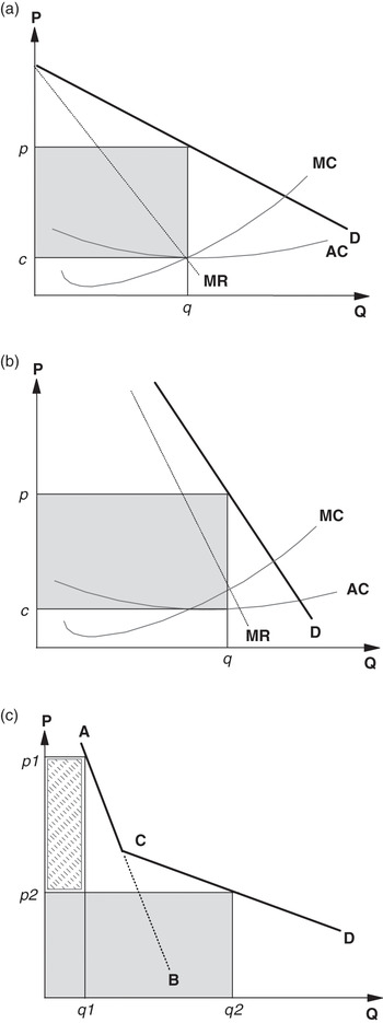
Figure 1.10. (a) Marginal costs and revenues, normal setting, (b) Demand becomes more inelastic and right-shifted, and (c) Consumers’ surplus under price discrimination.
Given that popular entertainment products feature one-of-a-kind talent (e.g., Elvis or Sinatra recordings) or brand-name products and services (e.g., Apple or Disney), the so-called competitive-monopolistic model of Figure 1.10a, in which many firms produce slightly differentiated products, is not far-fetched. The objectives for such profit-maximizing firms are to both rightward-shift and also steepen the demand schedule idealized by line D. A shift to the right represents an increase in demand at each given price.
Meanwhile, a schedule of demand that perhaps through promotional and marketing becomes more vertical (i.e., quantity demanded becomes less responsive to a change in price and becomes more price-inelastic) – enables a firm to reap a potentially large proportionate increase in profits as long as marginal costs are held relatively flat (Figure 1.10b). In all, the more substitutes that are available, the greater is the price elasticity of demand.
Look, for example, at what happens when a movie is made. The initial capital investment in production and marketing is risked without knowing how many units (including theater tickets, video sales and rentals, and television viewings) will ultimately be demanded. The possibilities range from practically zero to practically infinite.
Whatever the ultimate demand turns out to be, however, the costs of production and marketing, which are large compared with other, later costs, are mostly borne upfront. Come what may, the costs here are sunk (i.e., the money is already spent and is likely unrecoverable), whereas in many other manufacturing processes, the costs of raw materials and labor embedded in each unit produced (variable and marginal) may be relatively high and continuous over time.
In entertainment, the cost of producing an incremental unit (e.g., an extra movie print, DVD, or download) is normally miniscule as compared with the sunk costs, which should by this stage be irrelevant for the purpose of making ongoing strategic decisions. It may thus, accordingly, be sensible for a distributor to take a chance on spending a little more on marketing and promotion in an attempt to shift the demand schedule into a more price-inelastic and rightward position. Such inelastic demand is characteristic of products and services that
are considered to be necessities
have few substitutes
are a small part of the budget
are consumed over a relatively brief time, or are not used often.
Economists use estimates of elasticity (i.e., responsiveness) to indicate the expected percentage change in demand if there is a 1% change – up or down – in price or income (or some other factor). In the case of price, this can be stated as

All other things being equal, quantity demanded would normally be expected to rise with increases in income and decline with increases in price.26 For example, if quantity demanded declined 8% when price rose 4%, the price elasticity of demand would be −2.0. In theory, cross-elasticities of demand between goods and services that are close substitutes (a new Star Trek film versus a new Star Wars film), or complements to each other (movie admissions and sales of popcorn), might also be estimated. Such notions of elasticity suggest that it makes sense for firms to first increase the price markup on goods with the most inelastic demand (known as the Ramsey, or inverse elasticity pricing, rule).
In sum, when elasticity is greater than 1, price increases lead to decreases in revenue and vice versa. When elasticity is less than 1 (inelastic), increases in price lead to increases in revenues. And when elasticity equals 1, changes in price lead to no changes in revenues.
Elasticity: When prices are raised, revenues are …
| >1 | Lower |
| <1 | Higher |
| =1 | No change |
Similarly, elasticity with respect to income can be estimated for goods and services classifiable as luxuries, necessities, or inferiors.27 With luxuries, quantity demanded grows faster as income rises, and the income elasticity is greater than 1.0. For necessities, quantity demanded increases as income rises, but more slowly than income (elasticity 0.0 to 1.0). And for inferior goods, income elasticity is negative, with quantity demanded falling as income rises. By these measures, most entertainment products and services are either necessities or luxuries for most people most of the time (but with classification subject to change over the course of an economic or individual’s life-stage cycle).
That demand grows more slowly than income for needs (e.g., food, shelter, clothing) and more quickly for wants (e.g., entertainment, travel, recreation experiences) has been seen in most societies and nations. Figure 1.11 is based on per capita data from 116 countries and compares income elasticity estimates for a need category such as clothing to those for a want category such as recreation. From this it can be seen in the upper panel that needs demand grows at about the same pace as income, but that wants demand tends to rise at a higher rate than income: As countries become wealthier, people tend to spend proportionately more of their income on wants rather than needs.28

Figure 1.11. Needs (clothing) versus wants (recreation): income elasticity estimates in 116 countries, 2006.
Price Discrimination
If, moreover, a market for, say, airline or theater seats (see Chapter 13) can be segmented into first and economy classes, profits can be further enhanced by capturing what is known in economics as the consumers’ surplus – the price difference between what consumers actually pay and what they would be willing to pay. Such a price discrimination model extracts, without adding much to costs, the additional revenues shown in the darkened rectangular area of Figure 1.10c. The conditions that enable discrimination include
existence of monopoly power to regulate prices,
ability to segregate consumers with different elasticities of demand, and
inability of original buyers to resell the goods or services.
Such dynamic pricing or yield management strategies, as they are known, are commonly implemented in many different industries and may be beneficial to some consumers: For example, movie theaters may offer senior-citizen or matinee discounts that might not otherwise be available. And travelers willing to pay more for an airline ticket might be indirectly helping to reduce (i.e., subsidize) prices for those who are less willing. The extent to which subsidization of this type occurs will typically depend both on the industry-specific pricing conventions that have evolved over several business cycles and on the current intensity of competition in each consumer category.
Entertainment and media companies are especially able to advantageously apply price discrimination tactics by turning the introduction of important products and services into “events.” Releases of some new books, music tracks, films, game software, and openings of casinos, theme park attractions, sporting events, and television shows are typically “eventized” as a means of tapping into the willingness of some consumers and advertisers to pay premium prices.
To this end, economists have categorized discrimination into three types (degrees):
Public-Good Characteristics
Public (nonrival) goods are those that can be enjoyed by more than one person without reducing the amount available to any other person; providing the good to everyone else is costless. In addition, once the good exists, it is generally impossible to exclude anyone from enjoying the benefits, even if a person refuses to pay for the privilege. Such nonpayers are therefore “free riders.” In entertainment it is not unusual to find near-public-good characteristics: The marginal cost of adding one viewer to a television network program or of allowing an extra visitor into a theme park is not measurable. Spending on national defense or on programs to reduce air pollution is of this type. Public goods are thus non-rivalrous and non-excludable, whereas merit goods or services are provided by political decisions based on interpretations of need rather than ability or willingness to pay.
1.4 Personal-Consumption Expenditure Relationships
Recreational goods and services are those used or consumed during leisure time. As a result, there is a close relationship between demand for leisure and demand for recreational products and services.
As may be inferred from Table 1.6, NIPA data classify spending on recreation as a subset of total personal-consumption expenditures (PCEs). This table is particularly important because it allows comparison of the amount of leisure-related spending to the amounts of spending for shelter, transportation, food, clothing, national defense, and other items.29 For example, percentages of all PCEs allocated to selected major categories in 2018 were:
| Medical care | 16.9% |
| Housing | 18.3 |
| Transportation | 3.2 |
| All recreation | 6.8 |
| Food (excluding alcoholic beverages) | 7.2 |
| Clothing | 2.8 |
Table 1.6. PCEs for recreation in current dollars, selected categories, 1990–2018a
| Product or service by function | 1990 | 2005 | 2018 |
|---|---|---|---|
| Total recreation expenditures (goods + services)a | 227.3 | 633.9 | 957.8 |
| Percent of total PCEs | 5.4 | 6.7 | 6.8 |
| Amusement parks, campgrounds, etc. | 19.2 | 33.6 | 65.8 |
| Gambling (casino, track, lotteries) | 23.7 | 72.9 | 142.6 |
| Newspapers + periodicals | 21.6 | 36.1 | 47.8 |
| Books (edu + rec) | 16.2 | 36.8 | 32.7 |
| Cable TV + satellite services | 18.0 | 54.6 | 96.0 |
| Spectator amusements, total | 14.4 | 43.7 | 78.8 |
| Motion picture theaters | 5.1 | 9.7 | 15.7 |
| Spectator sportsb | 4.8 | 15.7 | 27.6 |
a In billions of dollars, except percentages. Represents market value of purchases of goods and services by individuals and nonprofit institutions. See Historical Statistics, Colonial Times to 1970, series H 878–893, for figures issued prior to 1981 revisions.
b Includes professional and amateur events and racetracks.
As may be seen in Figure 1.12, spending on entertainment services has trended gradually higher as a percentage of all PCEs, whereas percentages spent on clothing and food have declined.

Figure 1.12. Trends in percentage of total personal consumption expenditures in selected categories, 1980–2018.
That spending on total recreational goods and services responds to prevalent economic forces with a degree of predictability can be seen in Figure 1.13.30 Figure 1.14 illustrates that PCEs for recreation as a percentage of total disposable personal income (DPI) had held steady in a band of roughly 5.0% to 6.5% for most of the 80 years beginning in 1929. New heights can only be achieved as a result of a relatively lengthy business cycle expansion, increased consumer borrowing ratios, demographic and household formation influences, and the proliferation of leisure-related goods and services utilizing new technologies.

Figure 1.13. PCE for recreation as percentage of disposable income, 1929–2018.

Figure 1.14. PCE on recreation services as percentage of total PCE on recreation, 1959–2018.
Measurement of real (adjusted for inflation) per capita spending on total recreation and on recreation services provides yet another long-term view of how Americans have allocated their leisure-related dollars. Although the services subsegment excludes spending on durable products such as television sets, it includes movies, cable TV, sports, theater, commercial participant amusements, lotteries, and pari-mutuel betting. The percentage of recreation services spending is now above 40% of the total spent for all recreation (Figure 1.14), and a steeper uptrend in real per capita PCEs on total recreation and on recreation services beginning around 1960 is suggested by Figure 1.15.31

Figure 1.15. Real per-capita spending on total recreation and on recreation services, 1929–2018.
This apparent shift toward services, which is also being seen in other economically advanced nations, is a reflection of relative market saturation for durables, relative price-change patterns, and changes in consumer preferences that follow from the development of new goods and services. As such, even small percentage shifts of spending may represent billions of dollars flowing into or out of entertainment businesses. And for many firms, the direction of these flows may make the difference between prosperous growth or struggle and decay.
Because various entertainment sectors differ in responses to changing conditions, extreme across-the-board external shocks such as the globally devasting coronavirus pandemic of early 2020 – and also the degree of recession resistance or cyclicity of the entertainment industry relative to that of the economy at large – are not well depicted by such time series.32
For example, broadcasting revenues depend on advertising expenditures, which in turn relate to total corporate profits. Yet, movie and game segments might occasionally move opposite to macroeconomic trends and, to effectively study these business cycle relationships, less aggregated data must therefore be used. Measures of what is known as the gross national product (GNP), or of the more recent standard of gross domestic product (GDP), can thus provide only a starting point for further investigations.33
In addition, financial analysts of entertainment and media industries ought to recognize that prices of energy-sources have the potential to greatly affect overall personal-consumption expenditures and to significantly alter sector growth patterns.34 That’s because a price decline of $10 a barrel corresponds roughly to a 0.25 percentage point gain in GDP growth over the following year.
If the world cannot indeed continue to produce the low-cost energy that has enabled consumers everywhere to spend an increasing part of their incomes on leisure, entertainment, and travel pursuits, growth of spending for these categories is likely to be severely constrained and/or diminished.
Patterns of oil production and consumption for the world and for the U.S. are shown in Figures 1.16 and 1.17, respectively. The data suggest that world production might be leveling in the range of 36 to 40 billion barrels a year and that prices, particularly since the late 1990s, have been trending higher but with unpredictably volatile movements over the short run.35
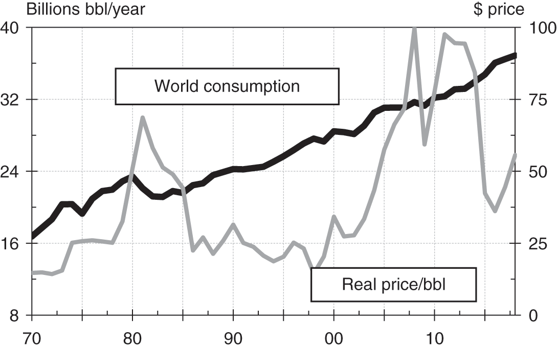
Figure 1.16. World crude oil consumption, billions of barrels per year, production closely tracks consumption, and real price per barrel in 2012 dollars, 1970–2018.

Figure 1.17. Crude oil production and consumption in the United States, billions of barrels/year, 1950–2018.
1.5 Price Effects
Prices are largely dependent on supply and demand factors related to particular goods or services. But economic policies and strategies implemented by governments and their central banks, which have the power to create or extinguish money and credit, often also have an important influence on whether overall prices are moving upward (inflation) or downward (deflation). Although notable episodes of inflation and deflation have occurred in many nations at many times in history, the tendency and preference is normally to allow prices to rise gradually (i.e., creep higher). As a result of compounding, though, even small annual increments in the wholesale (producer or PPI) and consumer price (CPI) indexes will over time significantly erode the purchasing power of a country’s currency, both internally and externally.
As a result, a dollar today reported as an average ticket price is not the same as one of yesterday or of ten years ago. In fact, in the United States, today’s dollar has the purchasing power of and is equivalent to perhaps only two or three cents of 100 years ago. And prices that are rising merely at a compound rate of around 3% a year will approximately double in a little more than 20 years.36 It is therefore important to be aware of such price effects when comparing data that are generated relatively far apart in time and to be careful when interpreting numbers that are stated as being “record-setting.” Indexes of this kind are also criticized as being misleading because they are frequently revised (in data and methodology) and poorly capture changes in quality and technology (i.e., so-called hedonic factors).37
Price trends as reported by the U.S. Bureau of Labor Statistics using the CPI and GDP deflator series appear in Figure 1.18. The main take-away from the heavy dark line (CPI-U) is that overall prices have more than tripled since 1980 (from around 82 to 250 in 2018). But it is also clear that admission prices for entertainment events have risen even faster than the CPI-U.

Figure 1.18. General price inflation indexes, CPI all items, admissions (movies, concerts, sporting events), 1984 = 100, and GDP deflator (2012 = 100), 1970–2018.
1.6 Industry Structures and Segments
Structures
Microeconomic theory suggests that industries can be categorized according to how firms make price and output decisions in response to prevailing market conditions. In perfect competition, all firms make identical products, and each firm is so small in relation to total industry output that its operations have a negligible effect on price or on quantity supplied. At the other idealized extreme is monopoly, in which there are no close substitutes for the single firm’s output, the firm sets prices, and there are barriers that prevent potential competitors from entering. A natural monopoly, moreover, occurs when it is impossible for potential competitors to “contest” a market because high fixed or sunk entry costs cannot be recouped (as prices converge to equal marginal costs and the monopolist’s economies of scale are large). Utility providers such as those distributing electricity, water, and cable television programming are typical examples.
In the real world, the structure of most industries cannot be characterized as being perfectly competitive or as monopolistic but as somewhere in between. One of those in-between structures is monopolistic competition, in which there are many sellers of somewhat differentiated products and in which some control of pricing and competition through advertising is seen. An oligopoly structure is similar, except that in oligopolies there are only a few sellers of products that are close substitutes and pricing decisions may affect the pricing and output decisions of other firms in the industry. Although the distinction between monopolistic competition and oligopoly is often blurred, it is clear that when firms must take a rival’s reaction to changes of price into account, the structure is oligopolistic. In media and entertainment, industry segments fall generally into the following somewhat overlapping structural categories:
| Monopoly | Oligopoly | Monopolistic competition |
|---|---|---|
| Cable TV | Movies | Books |
| Newspapers | Recorded music | Magazines |
| Professional sports teams | Network TV | Radio stations |
| Casinos | Toys and games | |
| Theme parks | Performing arts | |
| Internet service and social media networks | ||
| Video game producers/distributors |
These categories can then be further analyzed in terms of the degree to which there is a concentration of power among rival firms.38 A measure that is sensitive to both differences in the number of firms in an industry and differences in relative market shares – the Herfindahl–Hirschman Index – is frequently used by economists to measure the concentration of markets.39
Segments
The relative economic importance of various industry segments is illustrated in Figure 1.19(a–e), the trendlines of which provide long-range macroeconomic perspectives on entertainment industry growth patterns. These patterns then translate into short-run financial operating performance, as revealed by Table 1.7 and in which revenues, pretax operating incomes, assets, and cash flows (essentially earnings before taxes, interest, depreciation, and amortization) for a selected sample of major public companies are presented. This sample includes an estimated 80% of the transactions volume in entertainment-related industries and provides a means of comparing efficiencies in various segments.


Figure 1.19. PCEs of selected entertainment categories as percentages of total PCE on recreation, 1929–2018.
Table 1.7. Entertainment and media industry composite sample, 2014–2018
| Compound annual growth rates (%): 2014–2018 | |||||
|---|---|---|---|---|---|
| Industry segment | No. companies in sample | Revenues | Operating income | Assets | Operating cash flow |
| Broadcasting (television & radio) | 21 | 3.2 | 6.1 | 1.5 | 5.7 |
| Cable (video subscription services) | 19 | 8.4 | 6.8 | 6.8 | 3.2 |
| Filmed entertainment | 8 | 5.1 | 5.3 | 4.0 | 4.9 |
| Gaming (casinos) | 15 | 1.0 | 3.2 | 5.8 | 2.6 |
| Internet | 4 | 22.3 | 25.7 | 22.4 | 24.2 |
| Music recorded) | 6 | 15.1 | 37.4 | 7.5 | 36.7 |
| Publishing (books, mags, newspapers) | 17 | −1.7 | −1.1 | −2.7 | −1.5 |
| Theatrical exhibition | 5 | −0.9 | −2.9 | 2.3 | −0.3 |
| Theme parks | 6 | 6.6 | 11.3 | 6.0 | 10.5 |
| Toys | 10 | 5.3 | 3.2 | 7.5 | 26.9 |
| Total | 111 | ||||
| Total composite | ||||||
|---|---|---|---|---|---|---|
| Pretax return (%) on | ||||||
| Revenues | Assets | Revenuesb | Operating incomeb | Assetsb | Operating cash flowb | |
| 2018 | 24.7 | 13.8 | 746 | 184 | 1,336 | 269 |
| 2017 | 28.3 | −14.7 | 679 | 192 | 1,304 | 241 |
| 2016 | 29.3 | 14.6 | 594 | 174 | 1,191 | 234 |
| 2015 | 29.2 | 15.3 | 539 | 157 | 1,030 | 203 |
| 2014 | 30.3 | 15.9 | 516 | 156 | 985 | 196 |
| CARGa | 4.9 | −3.4 | 9.7 | 4.2 | 7.9 | 8.3 |
a Compound annual growth rate (%). Excluding Internet, growth would be much lower.
b In $ billions.
Cash flow is particularly important because it can be used to service debt, acquire assets, or pay dividends. In representing the difference between cash receipts from the sale of goods and services and cash outlays required in their production of the same, operating cash flow is usually understood to beoperating income (i.e., earnings) before deductions for interest, taxes, depreciation, and amortization (EBITDA). More recently and alternatively, operating income before depreciation and amortization (OIBDA) has been similarly applied.40
Although it has lost some analytical favor, cash flow (EBITDA) so defined has customarily been used as the basis for valuing all kinds of media and entertainment properties because the distortional effects of differing tax and financial structure considerations are stripped away. A business property can thus be more easily evaluated from the standpoint of what it might be worth to potential buyers.41 Also, a trend of declining EBIT margins (i.e., EBIT/revenues) always suggests that companies are finding it more difficult to convert revenues into free cash – a situation that if sustained leads ultimately to lower share valuations.
More immediately, it can be seen further that sampled entertainment industries generated revenues (on the wholesale level) of about $750 billion in 2018 and that annual growth between 2014 and 2018 averaged approximately 9.7% (largely led by Internet companies). In this, PCEs for casinos, cable, and theme parks have long been far larger than for movies. Over the same span, which included a continuing rebound from a long and deep recession, operating income rose at a compound rate of 4.2%, with total assets rising by 7.9%.
A thorough analysis of the composites shown in Table 1.7 would nevertheless further require consideration of many features of the business environment, including interest rates, antitrust policy attitudes, the trend of dollar exchange rates, and relative pricing power. This last factor is suggested by Figure 1.20, which compares the rise of the Consumer Price Index for two important entertainment segments (and also airfares) against the average of all items for all urban consumers (CPI-U). From this, it can be seen that cable television service prices have been rising at well above average rates.

Figure 1.20. Cable service and ticket price indexes compared to CPI (1983 = 100), 1983–2018. *Ticket admissions to movies, theaters, and concerts. Annual average airfares in U.S.
Although economists also examine various segments through the use of what are known as input–output (I/O) tables, such tables are more robustly employed in the analysis of industrial products and commodities and in travel and tourism (through use of Tourism Satellite Accounts) than they are in entertainment and media services. A typical I/O table in entertainment, for example, would indicate how much the advertising industry depends on spending by entertainment companies.42
Finally, an indexed comparison of the percentage of personal-consumption expenditures going to different segments reveals the effects of changes in technology and in spending preferences. Three such trends are reflected in Figure 1.21, which illustrates the indexed percentages of total PCEs going to movie admissions, spectator sports, and live entertainment (including legitimate theater, opera, and entertainments of nonprofit institutions, i.e., “performing arts”). Interestingly, since around 1980, live entertainment, with a boost from relatively rapidly rising prices, had until recently gained in comparison with the percentage spent on spectator sports. Meanwhile, though, the percentage of PCE spending for movie tickets has fallen sharply now that technology has provided many other diversions and/or alternative means of seeing films (e.g., on DVDs, satellite or cable television hookups, or Internet downloads and streams).

Figure 1.21. Indexed personal consumption expenditures on spectator sports, live entertainment, and movie theater admissions as a percentage of total PCEs (1929 = 1.0), 1929–2018.
1.7 Valuation Variables
Important as it is to understand the economic perspectives, it is ultimately the role of the financial analyst to condense this information into an asset valuation estimate. The key question for investors is whether the market is correctly pricing the assets of an industry or of a company. In attempting to arrive at an answer, analysts find that valuation of assets often involves as much art as it does science.
Valuation methods fall into three main categories of approaches, using discounted cash flows, comparison methods, and option-pricing models. Sometimes all three approaches are suitable and the results are judged. At other times, the characteristics of the asset to be valued are such that only one approach is used. In most cases, however, the central concept is discounted cash flow, which takes account of both the time value of money and risk.
Discounted Cash Flows
Given that the primary assets of media and entertainment companies are most often intangible and are embodied in the form of intellectual property rights, it makes sense to base valuations on the expected profits that the control of such rights might reasonably be expected to convey over time. Although it is not a flawless measure, estimated cash flow (or perhaps EBITDA) discounted back to a present value will usually well-reflect such profit potential as long as the proper discount rate is ascribed: Cash flow to equity (i.e., after interest expenses and principal payments) must use a cost of equity capital discount rate, whereas cash flow to the firm (i.e., prior to interest expenses and principal payments) would use a weighted average cost of capital (WACC) discount rate.
Essentially, the discounted cash flow approach takes the value of any asset as the net present value (NPV) of the sum of expected future cash flows as represented by the following formula:

where r is the risk-adjusted required rate of return (tied to current interest rates), CFt is the projected cash flow in period t, and n is the number of future periods over which the cash stream is to be received.
To illustrate this most simply, assume that the required rate of return is 9%, that the projected cash flows of a television program in each of the next three years are $3 million, $2 million, and $1 million, and that the program has no value beyond the third year. The NPV of the program would then be 3/(1.0 + 0.09) + 2/(1.0 + 0.09)2 + 1/(1.0 + 0.09)3 = 2.75 + 1.683 + 0.7722 = $5.205 million.
Comparison Methods
Valuations can also be made by comparing various financial ratios and characteristics of one company or industry to another. These comparisons will frequently include current price multiples of cash flows and estimates of earnings, shareholders’ equity, and revenue growth relative to those of similar properties. One of the best yardsticks for comparing global companies that report with different accounting standards is a ratio of enterprise value (EV) to EBITDA. Enterprise value, subject to adjustment for preferred shares and other off-balance-sheet items, equals total common shares outstanding times share price (i.e., equity capitalization) plus debt minus cash.
Of course, a ratio of price to cash flow, earnings, revenues, or some other financial feature should – but opportunistically may not – already inherently reflect the estimated discounted cash flow and/or salvage (terminal) values of an asset or class of assets. If cable systems are thus being traded at prices that suggest multiples of ten times next year’s projected cash flow, it is likely that most other systems with similar characteristics will also be priced at a multiple near ten.
In valuations of entertainment and media assets, this comparative-multiple approach is the one most often used, even though it might not fully capture what economists call externalities – those factors that would make a media property especially valuable to a specific buyer. Prestige, potential for political or moral influence, and access to certain markets are externalities that ordinarily affect media transaction prices.
Options
For assets that have option-like characteristics or that are traded infrequently, neither the discounted cash flow nor the price and ratio comparison approach can be readily applied. Instead, option-pricing models (e.g., the Black–Scholes model) that use contingent claim valuation estimates (of assets that pay off only under certain contingencies and assumed probability distributions) are usually employed. Specialized option contracts are regularly used in many entertainment and media segments (see Chapter 13).
With the possible exception of start-up Internet shares in the late 1990s, however, this approach has not normally been used in entertainment industry practice unless the asset to be valued is an option contract (e.g., a warrant, call, or put) or is a contract for marketing or distribution rights or for some form of intellectual property right (e.g., a patent).43
1.8 Concluding Remarks
This chapter has sketched the economic landscape in which all entertainment industries operate. It has indicated how hours at work, productivity trends, expected utility functions, demographics, and other factors can affect the amounts of time and money we spend on leisure-related goods and services. It has also provided benchmarks against which the relative growth rates and sizes of different industry segments or composites can be measured. For example, as a percentage of disposable income, U.S. PCEs for recreation – encompassing spending on entertainment as well as other leisure-time pursuits – first rose to well over 6% in the 1980s.
In all, entertainment is big business: At the wholesale level, it is now generating annual revenues exceeding $700 billion. Moreover, as measured in dollar value terms, entertainment has consistently been one of the largest net export categories (at least $20 billion in 2019) for the United States.44 Entertainment in all its forms has also always provided otherwise unavailable experiences to consumers and participants. Unlike many consumer products and services – which are intermediaries demanded as a means to reach another end (e.g., an airplane trip to visit customers) – entertainment is directly desired and consumed for the experiences and enjoyment that it inherently provides. As such, entertainment provides unique value as it reflects the interests and motivations, career trajectories, language, and political discourses of society at large.45
Technological innovation has obviously played an important role. It underlies the growth of productivity and thus of the relative supply of leisure time. Just as significantly, technological advances as tracked in Figure 1.22, have changed the way in which we think of entertainment products. Such products – whether movies, music, TV shows, video games, or words – must now be regarded as composite bits of “information” that can be produced, processed, and distributed as series of digits; coded bursts of zeros and ones that can represent sounds, pictures, and texts. Already, this has greatly altered the entertainment industry’s economic landscape and propelled sequential movement through time from the vaudeville of the 1880s, to films, then radio, broadcast TV, cable networks, and now, streaming.

Figure 1.22. Entertainment industry milestones, 1870–2018.
The past, then, is not a prologue – especially in a field where creative people are constantly finding new ways to turn a profit. The wide-ranging economic perspectives discussed in this chapter, however, provide a common background for all that follows.


