


1. Introduction
Acoustic streaming is a steady flow generated by Reynolds stresses in an acoustically oscillating fluid, either due to absorption in the main body of the fluid of an irrotational sound beam (for Eckart streaming or Quartz wind) or associated with the Stokes boundary layer adjacent to a solid boundary (Rayleigh's streaming, Rayleigh Reference Rayleigh1884). Quartz wind is generally observed in systems where the length scale is much longer than the wavelength whereas Rayleigh streaming is associated with a length scale of the same order of magnitude as the wavelength.
The typical geometry leading to the development of Rayleigh streaming flow is a resonator of length much larger than its transverse (or wall-normal) dimensions filled with compressible gas (initially at homogeneous pressure and temperature) submitted to an acoustic plane wave in the longitudinal (or axial, wall-parallel) direction. Figure 1 shows a schematic of the problem studied in the present paper corresponding to such a typical geometry. Rayleigh streaming flow is encountered for example in thermoacoustic devices, in which it is responsible for reducing the efficiency of the machines, especially for high powered devices. Indeed, the power density of a thermoacoustic device being roughly proportional to the square of the acoustic pressure amplitude, the streaming flow developing at high acoustic amplitudes is an important issue when optimizing thermoacoustic systems.

Figure 1. Typical problem geometry for Rayleigh streaming. (a) Axial acoustic velocity amplitude along the guide axis. (b) Associated streaming cells. The fluid domain under study in the present paper corresponds to the grey area.
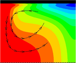
It is well established that, in the case of a plane standing wave at low amplitude, Rayleigh streaming is composed of toroidal so-called inner and outer vortices that have a half-wavelength spatial periodicity, the maximum axial streaming velocity being a quadratic function of the acoustic velocity amplitude at antinode. The inner vortices are slender and located near the walls, while the outer vortices develop in the core of the resonator. Figure 2 shows schematically the corresponding streamlines of the streaming flow in a half-wavelength resonator with acoustic velocity nodes at the extremities. The section shown is a longitudinal half-section between the axis (bottom) and the resonator wall (top). Heat is pumped by thermoacoustic effect initially in the near-wall region, from the acoustic velocity antinode towards the acoustic velocity nodes (Merkli & Thomann Reference Merkli and Thomann1975; Gopinath, Tait & Garrett Reference Gopinath, Tait and Garrett1998). It then diffuses transversely, resulting in a longitudinal temperature gradient. A colour map of the resulting isotherms of the mean temperature is displayed in the same figure. In this case, where the acoustic amplitude is low, the convective transport effect by the streaming flow is negligible and does not influence the organization of the thermal field.

Figure 2. Schematic of isothermal lines and streaming streamlines obtained in a half-wavelength resonator at low acoustic level. The section shown is a longitudinal half-section between the axis (bottom) and the resonator wall (top). Hot and cold regions are depicted.
For higher acoustic levels, Menguy & Gilbert (Reference Menguy and Gilbert2000) showed that the influence of inertial effects on the streaming flow is characterized by a reference nonlinear Reynolds number  $Re_{NL}=(M \times R/\delta _{\nu })^2$, where $M$ is the acoustic Mach number, $M=U_{ac}/c_0$, with $U_{ac}$ the maximum acoustic velocity on the channel axis and $c_0$ the initial speed of sound, $R$ being the half-width of the channel and $\delta _{\nu }$ the viscous boundary layer thickness. For $Re_{NL}=O(1)$, they found that the outer vortices are distorted by inertia, while the inner vortices are not affected. However, their study was limited to low values of $Re_{NL}$ (up to $Re_{NL}=6$) and they used the assumption of isentropic flow. Later, it was found, both experimentally by Thompson, Atchley & Maccarone (Reference Thompson, Atchley and Maccarone2005), Moreau, Bailliet & Valière (Reference Moreau, Bailliet and Valière2008), Reyt et al. (Reference Reyt, Daru, Bailliet, Moreau, Valière, Baltean-Carlès and Weisman2013) and Reyt, Bailliet & Valière (Reference Reyt, Bailliet and Valière2014) and numerically by Boluriaan & Morris (Reference Boluriaan and Morris2003), Reyt et al. (Reference Reyt, Daru, Bailliet, Moreau, Valière, Baltean-Carlès and Weisman2013) and Daru et al. (Reference Daru, Baltean-Carlès, Weisman, Debesse and Gandikota2013, Reference Daru, Reyt, Bailliet, Weisman and Baltean-Carlès2017a), that the longitudinal streaming velocity component along the axis, which is a sinusoidal function of the axial coordinate at low acoustic levels, becomes distorted as the acoustic level is increased. For high acoustic amplitudes, this distortion leads to the generation of counter-rotating additional vortices in the centre of the guide near the acoustic velocity antinodes, while in the near-wall region inner streaming vortices are only slightly modified.
In order to disentangle the physical phenomena responsible for the change of streaming pattern at high acoustic levels, the isentropic case was analysed in Daru et al. (Reference Daru, Weisman, Baltean-Carlès, Reyt and Bailliet2017b). A similar evolution of streaming pattern was observed, although for higher values of  $Re_{NL}$ than in experiments. It was shown numerically that inertial effects cannot be considered as the leading phenomenon to explain this evolution, which was rather attributed to nonlinear interactions between acoustic and streaming flows (Daru et al. Reference Daru, Reyt, Bailliet, Weisman and Baltean-Carlès2017a). The change of pattern was shown to occur when the radial streaming velocity becomes larger than the radial acoustic velocity.
Thermal effects on acoustic streaming flow were investigated analytically at low acoustic levels by Hamilton, Ilinskii & Zabolotskaya (Reference Hamilton, Ilinskii and Zabolotskaya2003) in channels/cylindrical guides of arbitrary width, where the base state (including temperature) is spatially uniform. They included variation of thermophysical gas properties with temperature (for several gases corresponding to several Prandtl numbers) and showed that thermal effects have a limited influence on the streaming flow for low amplitude acoustic waves.
The influence of an imposed longitudinal temperature gradient on acoustic streaming was considered theoretically by Rott (Reference Rott1974), Olson & Swift (Reference Olson and Swift1997) and Bailliet et al. (Reference Bailliet, Gusev, Raspet and Hiller2001) in the context of thermoacoustic devices, where parts of the resonator are maintained under large temperature gradients using heat exchangers. Thompson et al. (Reference Thompson, Atchley and Maccarone2005) showed experimentally the strong effect of a small thermoacoustically induced longitudinal temperature gradient on the acoustic streaming flow for values of the nonlinear Reynolds number  $Re_{NL}$ up to 20. The temperature gradient measured on the outside wall was small (up to $8\ \textrm {K}\ \textrm {m}^{-1}$, corresponding to a temperature difference across the streaming cell of $2.3\ \textrm {K}$). These streaming velocity measurements were not explained by theoretical studies in previously cited references.
The influence of an imposed transverse temperature gradient on Rayleigh streaming flow has been far less studied. Lin & Farouk (Reference Lin and Farouk2008) and Aktas & Ozgumus (Reference Aktas and Ozgumus2010) conducted some two-dimensional (2-D) numerical simulations with the two longitudinal walls maintained at different temperatures. They found that the outer symmetric vortices are distorted and merge to one vortex pattern for high values of the temperature difference (up to 60 K). Note that gravity is neglected in these studies. Nabavi, Siddiqui & Dargahi (Reference Nabavi, Siddiqui and Dargahi2008) studied experimentally the influence of differentially heated horizontal walls on acoustic streaming in a parallelepipedic channel of square cross-section. They applied a vertical bottom–top temperature difference (bottom wall hotter than the top wall) ranging from 0.8 K to 3 K and found that streaming patterns are greatly modified, both in shape and in value; the streaming velocity amplitude was increased when the temperature difference was increased. In their experiment the channel width is very large, of approximately  $400\delta _{\nu }$. However, in their study it is difficult to distinguish between buoyancy and inhomogeneity of temperature effects on the acoustic streaming flow. More recently Chini, Malecha & Dreeben (Reference Chini, Malecha and Dreeben2014) and Michel & Chini (Reference Michel and Chini2019) conducted theoretical studies of the acoustic streaming flow produced in a fluid with inhomogeneous background temperature and density, based on a multiple scale analysis. In Chini et al. (Reference Chini, Malecha and Dreeben2014), the streaming velocity is first order in Mach number, only induced by the transverse temperature gradient (it does not exist if the temperature gradient is zero) and the acoustic flow is non-dissipative. The authors called this streaming flow ‘baroclinic acoustic streaming’. The motivation was the study of high-intensity discharge lamps, where large temperature differences exist and a strong two-way coupling between the acoustic field and the streaming flow is to be expected. The analysis of Michel & Chini (Reference Michel and Chini2019) quantitatively explains the results of numerical simulations by Lin & Farouk (Reference Lin and Farouk2008) conducted for a temperature difference equal to 60 K.
Cervenka & Bednarrik (Reference Cervenka and Bednarrik2017) numerically studied in 2-D channels the evolution of streaming patterns with inhomogeneous background temperature, the inhomogeneity being introduced via varying prescribed temperature distribution along the resonator walls. They found that the resulting temperature heterogeneity in the direction perpendicular to the resonator axis has a great influence on the streaming field if the ratio of the channel width to the viscous boundary layer thickness is large enough. Depending on the conditions they showed that Rayleigh streaming can be enhanced (for the axis colder than the wall) or decreased (for the axis hotter than the wall), and that the streaming patterns can be considerably distorted even if the transverse temperature difference is small. In Cervenka & Bednarrik (Reference Cervenka and Bednarrik2018), the authors studied the added effect of convective heat transport on the streaming field in a cylindrical geometry. Their study was, however, limited to weak convective effects (and thus low values of  $Re_{NL}$), because their model was not numerically stable for values of the Reynolds number of the streaming flow, $Re_{NL}>4$. They explained that when a longitudinal temperature gradient is established in the tube due to the thermoacoustic effect, the streaming flow convects heat along the axis from the acoustic velocity node towards the antinode, causing the appearance of a transverse temperature gradient responsible for the modification of streaming patterns at high acoustic levels. Even though the mechanism for the distortion of streaming due to temperature effects was qualitatively identified, the effects need to be further quantified.
In the present study, the acoustically induced thermal effects on Rayleigh streaming flow in a waveguide at high acoustic amplitude are analysed by following a combined formal and phenomenological approach. In such a waveguide, a longitudinal temperature difference in the boundary layer near the wall is first created by thermoacoustic effect, as shown in figure 2. At high acoustic amplitude, convective transport effects by the streaming flow are no more negligible. Since transport occurs towards the acoustic velocity antinode near the waveguide axis and towards the acoustic velocity node near the wall, a large zone of transverse temperature stratification appears in the central part of the streaming cells (figure 3). Similar temperature distributions were observed in early numerical simulations by Gopinath & Mills (Reference Gopinath and Mills1994). This mean temperature reorganization results in spatial modification of the streaming patterns, and possibly the emergence of a new cell as previously observed experimentally and numerically by Thompson et al. (Reference Thompson, Atchley and Maccarone2005), Reyt et al. (Reference Reyt, Daru, Bailliet, Moreau, Valière, Baltean-Carlès and Weisman2013) and Daru et al. (Reference Daru, Baltean-Carlès, Weisman, Debesse and Gandikota2013).

Figure 3. Schematic of isothermal lines and streaming streamlines obtained in the waveguide at high acoustic levels. The white dashed-line rectangles indicate the transversely stratified temperature regions.
One of our aims is to identify the scaling parameters that predict this modification of streaming pattern. Following Cervenka & Bednarrik (Reference Cervenka and Bednarrik2018), we postulate that a major effect on the streaming flow patterns is to be attributed to the change of the temperature field distribution due to heat transport by convective effect. We thus expect that the streaming flow at high acoustic levels can be adequately studied theoretically by solving linear equations for both acoustic and streaming flows with an imposed background transversely stratified temperature distribution.
The transverse temperature difference observed in figure 3 is proportional to the longitudinal temperature difference observed in the boundary layer. The latter could be well approximated by the longitudinal temperature difference calculated on the inside boundary of the wall. Since the longitudinal temperature gradient due to thermoacoustic effect is expected to be small, the transverse variations of temperature under study here are supposed to be small.
Following the ideas presented above, the present study is divided in five sections. In § 2 the effect of a transversely stratified temperature distribution on the streaming flow is analysed in the plane case of low acoustic amplitude. The analytical model developed in Baltean-Carlès et al. (Reference Baltean-Carlès, Daru, Weisman, Tabakova and Bailliet2019) for isentropic flow is extended here to the case of variable mean temperature for a perfect gas. As in Baltean-Carlès et al. (Reference Baltean-Carlès, Daru, Weisman, Tabakova and Bailliet2019), the symbolic computational software Mathematica (Wolfram Research Inc. 2018) is used to solve the equations throughout this study. The plane case is addressed because analytical expressions are simpler and also we expect a behaviour very similar to the axisymmetric case (a cylindrical geometry would involve integration of products of Bessel function that do not have any known analytic expression). An important result is the quantification of the relevant similarity parameters, essential to provide guidelines in numerical and experimental studies.
In § 3 the wall temperature distribution is calculated from the combined thermoacoustic effect in the fluid, heat conduction in the wall and convection from the outside air. The maximum transverse temperature difference to be expected due to convective transport can then be estimated, since it is proportional to the maximum longitudinal temperature difference (figure 3).
These results are then combined in § 4 to exhibit a new criterion characterizing the transition in streaming pattern.
This criterion is shown in § 5 to be in good agreement with the experimental results in the literature reported by Thompson et al. (Reference Thompson, Atchley and Maccarone2005) and Reyt et al. (Reference Reyt, Bailliet and Valière2014). It thus provides the first quantitative explanation of the evolution of streaming observed in these experiments. Moreover, it explains for the first time the influence of thermal boundary conditions observed in previous experiments.
2. Analytical solution for Rayleigh streaming flow under a transverse gradient of temperature
In this section the effect of a transverse gradient of temperature on acoustic streaming is investigated. As stated in the Introduction, previous studies by Chini et al. (Reference Chini, Malecha and Dreeben2014), Cervenka & Bednarrik (Reference Cervenka and Bednarrik2017, Reference Cervenka and Bednarrik2018) and Michel & Chini (Reference Michel and Chini2019) have already shown that transverse variations of the fluid temperature lead to drastic changes in the streaming flow structure. Our goal here is to quantify these changes in Rayleigh streaming with respect to the geometrical parameters of the guide, thermophysical characteristics of the gas and transverse temperature difference.
The configuration under study consists in a waveguide filled with a perfect gas initially at rest. A plane standing acoustic wave of angular frequency  $\omega$ is installed inside the channel. The channel has a length $L$ and a half-width $R$. Figure 1 shows the flow domain, the symmetry conditions and the thermal boundary conditions. The reference state corresponds to uniform temperature $T_0$, density $\rho _0$, pressure $p_0$. The corresponding sound velocity is $c_0=\sqrt {\gamma p_0/\rho _0}$, with $\gamma$ the ratio of specific heats. The angular frequency is equal to $\omega _0$ corresponding to the acoustic standing wave resonating at its first mode along $x$ (so-called $\lambda /2$ mode), in the case of a non-viscous gas ( $\omega _0={{\rm \pi} c_0}/{L}$). The channel length is large compared to its width, $L \gg R$. The effects of gravity are not included in this study.
In the following, coordinates  $x$,
$x$,  $y$ and velocity components $u$,
$u$,  $v$ correspond respectively to the axial and transverse directions. The origin is at the centre of the channel. Pressure, density and temperature are denoted respectively $p$,
$p$,  $\rho$ and $T$. The following non-dimensional quantities are used:
 \begin{equation} \hat{y}=y/\delta_\nu, \quad \hat{x}=x/L, \quad \hat{R}=R/\delta_\nu, \quad \hat{L}=L/\delta_\nu, \end{equation}
where  $\delta _\nu =\sqrt {{2 \mu }/({\rho _0 \omega _0})}$ is the oscillating viscous boundary layer thickness, $\mu$ being the dynamic viscosity of the gas. For symmetry reasons only a half-channel is considered, that is, the velocity and temperature fields are calculated and shown for $-1/2 \leqslant \hat {x} \leqslant 1/2$ and $0 \leqslant \hat {y} \leqslant \hat {R}$ only. The propagation of a low amplitude plane acoustic wave is associated with a perturbation of the initial state (defined by $p_0$, $\rho _m$ and $T_m$) for the fluid yielding
 \begin{equation} p=p_0+p' , \quad u=u' , \quad v=v', \quad T=T_m+T' , \quad \rho=\rho_m+\rho' . \end{equation}
 We introduce the complex acoustic amplitudes  $\tilde {p}$, $\tilde {\rho }$, $\tilde {u}$, $\tilde {v}$, $\tilde {T}$ such that $p'=Re(\tilde {p} \exp (\textrm {i} 2 {\rm \pi}\hat {t}))$, $\rho '=Re(\tilde {\rho } \exp (\textrm {i} 2 {\rm \pi}\hat {t}))$, etc., where $\hat {t}={\omega _0}/({2 {\rm \pi}}) t$ is the non-dimensional time.
Using Reynolds decomposition, any fluid variable  $\phi$ is separated into a fluctuating, periodic, component $\phi '$, and a steady component $\bar {\phi }$ according to
 \begin{equation} \phi =\bar{\phi}+\phi', \end{equation}
where the overline denotes the average over an acoustic period. It should be noted that the averaged product of variables  $\phi$ and $\psi$ writes
 \begin{equation} \overline{\phi \psi} = \bar{\phi}\ \bar{\psi} +\overline{\phi' \psi'}. \end{equation}
 It is assumed that the transport properties of the gas such as specific heats  $c_p$ and $c_v$, heat conductivity $k$ and viscosity $\mu$ are constant, since the effect of their variation with temperature is expected to be very small for the range of temperature variations under study. Only gases with Prandtl number $Pr <1$ are considered here (where $Pr= {\mu c_p}/{k}$).
The wall temperature is constant and equal to the reference temperature  $T_0$. The temperature difference in the fluid between the wall and the resonator axis is noted ${\rm \Delta} T$. As stated before, for our application, ${\rm \Delta} T$ is supposed to be small, that is $\varTheta =({{\rm \Delta} T}/{T_0}) \ll 1$. This corresponds to temperature differences of few degrees when working at room temperature. In the following, terms in $O(\varTheta ^2)$ and smaller will be neglected. Axial symmetry for temperature induces ${\partial T}/{\partial \hat {y}}|_{\hat {y}=0}=0$.
The initial temperature distribution is taken as the simplest function  $T_m(\hat {y})$ satisfying both boundary and symmetry conditions
 \begin{equation} \frac{T_m}{T_0}=1+\varTheta \left(1-\frac{\hat{y}^2}{\hat{R}^2}\right)=f(\hat{y}). \end{equation}
 This temperature distribution can be obtained by adding a source term  $Q=2 k ({{\rm \Delta} T}/{R^2})$ in the energy equation, which in the absence of fluid motion reduces to $k ({\partial ^2 T_m}/{\partial x^2}+{\partial ^2 T_m}/{\partial y^2})= - Q$.
The equation of state for a perfect gas is  $p=r \rho T$ (where $r=c_p-c_v$), resulting for the average state in the approximate equation $p_0=r \rho _m T_m$, where the averaged fluctuating term $\overline {\rho ' T'}$ is neglected (since it is second order in Mach number).
The temperature distribution (2.5) induces a density distribution in order to satisfy the equation of state  $p_0=r \rho _m T_m$, and the average density $\rho _m (\hat {y})$ takes the form
 \begin{equation} \frac{\rho_m}{\rho_0}=\frac{1}{\,f(\hat{y})} . \end{equation}
The imposed temperature distribution also induces a modification of the acoustic quantities. The following paragraph is devoted to establish the modified expression of the acoustic field.
2.1. Acoustics
Since  $R \ll L$ the acoustic wave is plane. For the configuration under study $(\partial u'/\partial x)/(\partial u'/\partial y) $ scales as $\delta _\nu /\lambda \ll 1$, therefore ${\partial ^2 u'}/{\partial x^2} \ll {\partial ^2 u'}/{\partial y^2}$ and the first-order equations governing the acoustics are
 \begin{equation} \left.\begin{gathered} \frac{c_0}{2} \frac{\partial \rho'}{\partial \hat{t}}+ \rho_m \frac{\partial u'}{\partial \hat{x}}+\hat{L}\frac{\partial }{\partial \hat{y}}(\rho_m v')=0,\\ \rho_m \frac{ c_0}{2} \frac{\partial u'}{\partial \hat{t}}+ \frac{\partial p'}{\partial \hat{x}}=\rho_0 \frac{\rm \pi}{2} c_0 \frac{\partial^2 u'}{\partial \hat{y}^2},\\ \frac{\partial p'}{\partial \hat{y}}=0,\\ \rho_m \frac{\partial T'}{\partial \hat{t}}=\rho_0 \frac{\rm \pi}{Pr} \frac{\partial^2 T'}{\partial \hat{y}^2}+ \frac{1}{c_p}\frac{\partial p'}{\partial \hat{t}}. \end{gathered}\right\} \end{equation}
The first-order equation of state for density is
 \begin{equation} \frac{\rho'}{\rho_m}=\frac{p'}{p_0}-\frac{T'}{T_m}.\end{equation}
 The boundary and symmetry conditions for  $u'$,
$u'$,  $v'$ and $T'$ with respect to $\hat {y}$ give
 \begin{equation} \left.\begin{gathered} u'=0 \ \mbox{at}\ \hat{y}=\hat{R};\quad \frac{\partial u'}{\partial \hat{y}}=0 \ \mbox{at} \ \hat{y}=0,\\ v'=0 \ \mbox{at}\ \hat{y}=\hat{R}\quad \mbox{and}\quad \textrm{at}\ \hat{y}=0,\\ T'=0 \ \mbox{at}\ \hat{y}=\hat{R};\quad \frac{\partial T'}{\partial \hat{y}}=0 \ \mbox{at} \ \hat{y}=0. \end{gathered}\right\} \end{equation}
Considering that the acoustic wave is plane, the acoustic pressure amplitude  $\tilde {p}$ is supposed to be real and of the form
 \begin{equation} \tilde{p}= \rho_0 c_0 U_{ac} \sin({\rm \pi} \hat{x}). \end{equation}
The complex acoustic velocity amplitude  $\tilde {u}$ should verify the following equation:
 \begin{equation} \textrm{i} \tilde{u}-\frac{1}{2} \,f(\hat{y}) \frac{\partial^2 \tilde{u}}{\partial \hat{y}^2}= - \frac{1}{\rho_0 {\rm \pi}c_0}\,f(\hat{y}) \frac{\textrm{d} \tilde{p}}{\textrm{d}\kern0.06em \hat{x}} . \end{equation}
Because we were not able to find an exact formal solution for (2.11), the following approximate solution is proposed  $\tilde {u}=\tilde {u}_1f(\hat {y})$, where $\tilde {u}_1$ is the solution of
 \begin{equation} \textrm{i} \tilde{u}_1-\frac{1}{2} \frac{\partial^2 \tilde{u}_1}{\partial \hat{y}^2}= - \frac{1}{\rho_0 {\rm \pi}c_0} \frac{\textrm{d} \tilde{p}}{\textrm{d}\kern0.06em \hat{x}}, \end{equation}
that is the usual equation written when temperature is homogeneous. The corresponding solution for  $\tilde {u}_1$ is
 \begin{equation} \tilde{u}_1=\frac{\textrm{i}}{\rho_0 {\rm \pi}c_0} (1-\exp({(1+{{\rm i}})(\hat{y}-\hat{R})})) \frac{\textrm{d}\tilde{p}}{\textrm{d}\kern0.06em \hat{x}} . \end{equation}
Therefore  $\tilde {u}$ is equal to
 \begin{equation} \tilde{u}=\textrm{i} U_{ac} \,f(\hat{y})(1-\exp({(1+{{\rm i}})(\hat{y}-\hat{R})})) \cos({\rm \pi} \hat{x}) . \end{equation}
In order to test the validity of this approximation,  $\tilde {u}$ is replaced in (2.11), resulting in
 \begin{equation} \textrm{i} \tilde{u}-\frac{1}{2} \,f(\hat{y}) \frac{\partial^2 \tilde{u}}{\partial \hat{y}^2}= - \frac{1}{\rho_0 {\rm \pi}c_0}\,f(\hat{y}) \frac{\textrm{d} \tilde{p}}{\textrm{d}\kern0.06em \hat{x}}\left[1 +\delta(\varTheta, \hat{y},\hat{R})\right], \end{equation}
with  $\delta (\varTheta , \hat {y},\hat {R})= {\varTheta }/{\hat {R}^2}(-\textrm {i}+ \exp ({(1 +{{\rm i}}) (\hat {y}-\hat {R} )}) (\textrm {i}+\hat {R}^2-2(1-{\rm i})\hat {y} -\hat {y}^2))$.
The residual function  $\delta$ (shown in figure 4) has maximum modulus values for $\hat {y}=\hat {R}$, where $|\delta (\varTheta , \hat {R},\hat {R})|=2 \sqrt {2}({\varTheta }/{\hat {R}})$. Therefore, $|\delta (\varTheta , \hat {R},\hat {R})|$ remains less than $8 \times 10^{-3}$ for $0\leqslant \varTheta \leqslant 5/T_0$ ( $T_0=294\ \textrm {K}$) and $6 \leqslant \hat {R} \leqslant 200$. The applications under study in the present paper correspond to a small enough transverse temperature gradient and large enough guides to validate the approximation of the solution of (2.11) by (2.14).

Figure 4. Values of  $|\delta (\varTheta , \hat {R},\hat {R})|$; $\varTheta$ varies between 0 and 5/294, $\hat {R}$ between 6 and 200.
The oscillating temperature amplitude  $\tilde {T}$ verifies an equation similar to (2.11)
 \begin{equation} \textrm{i} \tilde{T}-\frac{1}{2 Pr} \,f(\hat{y}) \frac{\partial^2 \tilde{T}}{\partial \hat{y}^2}= \textrm{i} \frac{1}{\rho_0 c_p}\,f(\hat{y}) \tilde{p} .\end{equation}
Following the same approach as for the velocity amplitude, the solution is approximated as
 \begin{equation} \tilde{T}= \frac{1}{\rho_0 c_p}\,f(\hat{y}) (1-\exp({(1+{{\rm i}})\sqrt{Pr}(\hat{y}-\hat{R})})) \tilde{p} . \end{equation}
 Finally the transverse acoustic velocity amplitude  $\tilde {v}$ is calculated by integrating the continuity equation. The density amplitude $\tilde {\rho }$ is obtained from the equation of state
 \begin{equation} \frac{\tilde{\rho}}{\rho_m}=\frac{\tilde{p}}{p_0}-\frac{\tilde{T}}{T_m} . \end{equation}
Substituting (2.18) in (2.7a) gives the following differential equation for  $\tilde {v}$:
 \begin{equation} \hat{L}\,f(\hat{y}) \frac{\partial }{\partial \hat{y}}\left(\frac{1}{\,f(\hat{y})} \tilde{v}\right)=-\textrm{i} {\rm \pi}c_0 \left(\frac{\tilde{p}}{p_0}-\frac{1}{\,f(\hat{y})}\frac{\tilde{T}}{T_0}\right)-\frac{\partial \tilde{u}}{\partial \hat{x}} . \end{equation}
 The resulting expression for  $\tilde {v}$ provided by formal integration is very lengthy and will not be given here. Instead, figure 5 shows the transverse profiles of $\tilde {u}$ and $\tilde {v}$ for ${\rm \Delta} T=0$ and $5$ K. This figure shows that the two velocity component profiles are not modified inside the boundary layer. Outside the boundary layer, the axial velocity amplitude is barely modified (maximum variation of $5/294=1.7$ %) while the transverse velocity amplitude varies by a maximum of approximately 15 %. We have previously shown in Daru et al. (Reference Daru, Reyt, Bailliet, Weisman and Baltean-Carlès2017a) that such variations on the transverse velocity amplitude can lead to significant modifications of the streaming flow. In that previous study, the modification of the transverse velocity was identified as coming from the nonlinear interaction between streaming and acoustic flows. The present development confirms that, as shown by Chini et al. (Reference Chini, Malecha and Dreeben2014) and Michel & Chini (Reference Michel and Chini2019), another source of modification of transverse acoustic velocity and thus of acoustic streaming is the presence of a transverse temperature gradient, via a baroclinic mechanism.

Figure 5. Transverse profiles of axial ( $\hat {x}=0$, a) and transverse ( $\hat {x}=-1/2$, b) acoustic velocities ( $\textrm {m}\ \textrm {s}^{-1}$), $\hat {R}=50$. With ${\rm \Delta} T=5\ \textrm {K}$ (solid), ${\rm \Delta} T=0\ \textrm {K}$ (dashed) and $U_{ac}=1\ \textrm {m}\ \textrm {s}^{-1}$, air at standard conditions.
As can be seen in figure 5, the influence of the inhomogeneity of temperature is less apparent on the axial acoustic velocity than on the radial one. However, as shown in the next section, both components have comparable resulting influence on the streaming velocity.
2.2. Streaming flow
In this section, the effect of a small transverse temperature gradient on acoustic streaming is investigated using the acoustic quantities calculated in the previous section.
Using the hypothesis that  ${\partial ^2 \bar {u}}/{\partial x^2} \ll {\partial ^2 \bar {u}}/{\partial y^2}$, the Navier–Stokes equations are averaged in time over one acoustic period, linearized and simplified as
 \begin{equation} \left.\begin{gathered} \frac{\partial }{\partial \hat{x}}(\rho_m \bar{u})+\hat{L} \frac{\partial }{\partial \hat{y}}(\rho_m \bar{v})=-\frac{\partial}{\partial \hat{x}}(\overline{\rho'u'})-\hat{L} \frac{\partial}{\partial \hat{y}}(\overline{\rho'v'}), \\ \rho_0\frac{\rm \pi}{2} c_0 \frac{\partial^2 \bar{u}}{\partial \hat{y}^2}= \frac{\partial \bar{p}}{\partial \hat{x}}+ \frac{\partial}{\partial \hat{x}}(\rho_m \overline{u'u'})+ \hat{L} \frac{\partial}{\partial \hat{y}}(\rho_m \overline{ u'v'}) , \\ \frac{\partial \bar{p}}{\partial \hat{y}}=0, \end{gathered}\right\} \end{equation}
where  $\bar {u}$, $\bar {v}$ and $\bar {p}$ are the averaged velocity components and pressure, and the fluid mean density $\rho _m$ is given by (2.6). The averaged terms on the right-hand side of system (2.20) are the averaged products (Reynolds stresses) of acoustic quantities. They are the sources of streaming. In the present study, two of the three sources of streaming that were investigated in Baltean-Carlès et al. (Reference Baltean-Carlès, Daru, Weisman, Tabakova and Bailliet2019) are taken into consideration. This is because the third source is negligible for the configuration presently studied.
The boundary conditions for  $\bar {u}$ and $\bar {v}$ are
 \begin{equation} \left.\begin{gathered} \bar{u}=0 \ \mbox{at}\ \hat{y}=\hat{R}; \quad \frac{\partial \bar{u}}{\partial \hat{y}}=0 \ \mbox{at} \ \hat{y}=0,\\ \bar{v}=0 \ \mbox{at}\ \hat{y}=0 \quad \mbox{and}\quad \hat{y}=\hat{R},\\ \int_0^{\hat{R}} \rho_m \bar{u} \,\mbox{d}\hat{y}=0. \end{gathered} \right\} \end{equation}
The third condition in (2.21a–c) is obtained by integrating the continuity equation in (2.20) over the half-width of the channel.
Following Westervelt (Reference Westervelt1953), we take the curl of the momentum equations, which eliminates pressure, and use the assumption  $1/L \partial \bar{v}/ \partial \hat{x} \ll 1/\delta_\nu \partial \bar{u}/ \partial \hat{y}$, to obtain
 \begin{equation} \frac{\rm \pi}{2} c_0 \frac{\partial^3 \bar{u}}{\partial \hat{y}^3}= \frac{\partial }{\partial \hat{y}}\left( \frac{1}{\,f(\hat{y})}\frac{\partial (\overline{u'u'})}{\partial \hat{x}} \right)+ \hat{L} \frac{\partial^2 }{\partial \hat{y}^2}\left(\frac{1}{\,f(\hat{y})}\overline{u'v'}\right). \end{equation}
 Since the formulae are very lengthy, formal integration is simplified for large guides and a small transverse temperature gradient by neglecting terms proportional to  $\textrm {e}^{- \hat {R}}$ and smaller as well as terms quadratic in $\varTheta$ and smaller.
The solution of the problem given by (2.22) is the superposition of solutions associated with each source term. Therefore, in the following, the two problems associated with the two source terms in (2.22) are solved successively.
2.2.1. First problem
The equation to be solved for the axial streaming velocity corresponding to the first source term is
 \begin{equation} \frac{\rm \pi}{2} c_0 \frac{\partial^3 \bar{u}_1}{\partial \hat{y}^3}= \frac{\partial }{\partial \hat{y}}\left( \frac{1}{\,f(\hat{y})}\frac{\partial (\overline{u'u'})}{\partial \hat{x}} \right). \end{equation}
The solution results in a lengthy expression not developed here. However, along the axis when smaller terms can be neglected the solution can be simplified into
 \begin{equation} \frac{\bar{u}_1(\hat{x},0)}{\bar{u}_R}= \frac{2}{3}-\frac{5}{\hat{R}}-\frac{4}{45}\varTheta \hat{R}^2 , \end{equation}
where the reference Rayleigh solution has been used for normalization
 \begin{equation} \bar{u}_R=-\frac{3}{16}\frac{U_{ac}^2}{c_0} \sin(2 {\rm \pi}\hat{x}) . \end{equation}
2.2.2. Second problem
The equation to be solved for the axial streaming velocity corresponding to the second source term writes
 \begin{equation} \frac{\rm \pi}{2} c_0 \frac{\partial^3 \bar{u}_2}{\partial \hat{y}^3}= \hat{L} \frac{\partial^2 }{\partial \hat{y}^2}\left(\frac{1}{\,f(\hat{y})}\overline{u'v'}\right) . \end{equation}
Again, only the streaming velocity along the axis is given here, neglecting smaller terms and normalizing with Rayleigh's solution; it writes
 \begin{align} \frac{\bar{u}_2(\hat{x},0)}{\bar{u}_R}&= \frac{1}{3}+\frac{2}{3}\frac{(\gamma -1)\sqrt{Pr}}{1+Pr}\nonumber\\ &\quad + \frac{1}{6 \hat{R}}\left[ 1+\frac{2(\gamma-1)}{Pr^{3/2}(1+Pr)^2}\left( 3 +5 Pr+6 Pr^{3/2}-8 Pr^2-4 Pr^3 \right) \right] +\frac{2}{45}\varTheta \hat{R}^2. \end{align}
Note that the additional term in  $\varTheta$ is of a sign opposite to the one in the first problem.
2.2.3. Total axial streaming velocity
The total axial streaming velocity is given by  $\bar {u}=\bar {u}_1+\bar {u}_2$, resulting along the axis in
 \begin{align} \frac{\bar{u}(\hat{x},0)}{\bar{u}_R}&= 1+\frac{2}{3}\frac{(\gamma -1)\sqrt{Pr}}{1+Pr} -\frac{29}{6}\frac{1}{\hat{R}}-\frac{2}{45}\varTheta \hat{R}^2\nonumber\\ &\quad + \frac{1}{6 \hat{R}}\left[ \frac{2(\gamma-1)}{Pr^{3/2}(1+Pr)^2}(3 +5 Pr+6 Pr^{3/2}-8 Pr^2-4 Pr^3) \right] . \end{align}
The first two terms in the right-hand side of (2.28) correspond to the solution given by Rott (Reference Rott1974), and also to that given in Hamilton et al. (Reference Hamilton, Ilinskii and Zabolotskaya2003) in the limit of wide channels. This expression depicts the huge effect of transverse temperature variation on the streaming velocity field, due to the term that varies in  $\hat {R}^2$. Note that, under the hypotheses of the present study, the order of magnitude of the term $\frac {2}{45}\varTheta \hat {R}^2$ is up to unity. This term, proportional to $\varTheta \hat {R}^2$, may be at the origin of the generation of an additional vortex. Expression (2.28) shows that this additional vortex rotates in the same direction as the Rayleigh outer cell if $\varTheta$ is negative (corresponding to the fluid near the axis being colder than the fluid near the wall), increasing the global amplitude of the outer streaming flow. In the opposite case, where $\varTheta \geqslant 0$ (fluid near the axis hotter than near the wall), the additional cell rotates in the opposite direction, thus decreasing the outer streaming flow. This phenomenon can eventually result in streaming flowing reversely with respect to the usual Rayleigh streaming flow. Unlike the case where $\varTheta = 0$, for which the fluctuating velocity field is rotational only in the boundary layer, when $\varTheta \ne 0$ it is rotational in the whole fluid which induces a baroclinic-type streaming flow as shown in Chini et al. (Reference Chini, Malecha and Dreeben2014) and Michel & Chini (Reference Michel and Chini2019). In our case, there are two mechanisms creating streaming: one inside the boundary layer, as for classical Rayleigh streaming, and one related to the transverse temperature gradient. This is consistent with findings by Cervenka & Bednarrik (Reference Cervenka and Bednarrik2017, Reference Cervenka and Bednarrik2018). The interest of the present work is to provide simple expressions that quantify this phenomenon in cases of small temperature gradients.
Let us consider the condition for reversing streaming flow for two guide widths, with air at standard conditions ( $T_0=294$ K). Figure 6 shows the axial streaming velocity normalized with the reference Rayleigh solution $\bar {u}_R$ as a function of $\hat {y}$ for $\hat {R}=50$ and for four values of $\varTheta$ ( $\varTheta \times T_0=0,1, 2,3\ \textrm {K}$). In this case, a temperature gradient of a few degrees changes drastically the velocity, which becomes negative on the axis. Figure 7 shows analogous curves for a wider guide, corresponding to $\hat {R}=150$, and for four values of $\varTheta$ ( $\varTheta \times T_0=0,0.1, 0.2,0.3\ \textrm {K}$). Here, the effect of temperature is even more important: only a few tenths of a degree is enough to reverse the velocity on the axis. Comparing these two figures illustrates the fact that, as $\hat {R}$ increases, the ${\rm \Delta} T$ needed to reverse the streaming flow on the axis decreases since it is inversely proportional to $\hat {R}^2$.

Figure 6. Transverse profiles of axial streaming velocity normalized by Rayleigh streaming for different transverse temperature gradients. Here,  $\hat {R}$ =50, $\hat {x}=-1/4$, $\varTheta$ varies between 0 (solid line) and $3$K
$3$K $/T_0$ (dotted line).

Figure 7. Transverse profiles of axial streaming velocity normalized by Rayleigh streaming for different transverse temperature gradients. Here,  $\hat {R}$ =150, $\hat {x}=-1/4$, $\varTheta$ varies between 0 (solid line) and $0.3$K $/T_0$ (dotted line).
2.2.4. Comparison with direct numerical simulation
To validate the simplifications made in our analytical study, we run a numerical simulation using the code described in Daru et al. (Reference Daru, Baltean-Carlès, Weisman, Debesse and Gandikota2013), that solves the complete compressible Navier–Stokes equations. In the code, the acoustic wave is created by shaking the channel periodically in the axial direction. The displacement amplitude is small in order to remain in the monofrequency acoustic regime. An initial temperature profile (2.5) is imposed, and maintained by adding the corresponding source term in the energy equation. The configuration used in this case corresponds to an acoustic wave frequency of  $20\,000$ Hz in a plane channel of width $\hat {R}=50$, filled with air at standard conditions ( $T_0=294$ K). The results are shown in figure 8, showing the normalized axial streaming velocity along the transverse direction, in the middle of the streaming cells $\hat {x}=-\frac {1}{4}$. A very good agreement between numerical and analytical solutions is observed, showing that our analytical approach gives a very good approximation to the complete problem.

Figure 8. Comparison between numerical simulation and analytical solution,  $\hat {R}$ =50, $\hat {x}=-1/4$; (a) $\varTheta =3\ \textrm {K}/T_0$, (b) $\varTheta =5\ \textrm {K}/T_0$.
3. Temperature distribution along the resonator wall
In order to describe the interaction between acoustic streaming and thermal effects in a standing waveguide, as stated in the Introduction, we now focus on the resonator mean wall temperature and its longitudinal variation. The wall temperature distribution is a result of the combination of thermoacoustic effect in the fluid, heat conduction in the wall and possible convection by the outside air.
The channel walls are assumed to be of thickness  $w$ and made with a material of thermal conductivity $k_s$, density $\rho _s$ and specific heat $c_s$. The initial temperature field is supposed to be uniform in the fluid, in the wall and outside the waveguide, that is $T=T_0$ everywhere. Three different thermal boundary conditions on the resonator wall are encountered in experimental studies: isothermal, uncontrolled and insulated. In the following, the temperature distribution along the wall is set first for the so-called ‘isothermal’ condition, where the outer side of the wall is maintained at temperature $T_0$. Secondly, the influence of convection outside the guide is taken into account by using a heat transfer coefficient. This second case should mimic the so-called ‘uncontrolled’ boundary conditions in experimental studies. The third boundary condition encountered in experimental studies is the insulated condition. In experiments, there always remains a very small heat exchange with the outside air. Therefore, this condition is equivalent to an uncontrolled boundary condition with a much smaller effective wall conductivity.
3.1. Isothermal condition
In the isothermal case, the temperature of the fluid outside the guide is supposed constant and equal to  $T_0$. The equation governing heat transfer by the fluid inside the waveguide is written by averaging over an acoustic period and neglecting terms smaller than second order in $M$ (Swift Reference Swift1988)
 \begin{equation} \frac{\partial}{\partial \hat{x}}\overline{u' T'} + \hat{L}\frac{\partial}{\partial \hat{y}}\overline{v' T'}=\frac{1}{2}{\rm \pi} c_0 \frac{1}{Pr} \frac{\partial^2 \bar{T}}{\partial \hat{y}^2}. \end{equation}
 Integrating (3.1) from 0 to  $\hat {R}$ yields
 \begin{equation} \int_0^{\hat{R}} \frac{\partial}{\partial \hat{x}}\overline{u' T'} \,{\textrm{d} y} =\frac{1}{2}{\rm \pi} c_0 \frac{1}{Pr} \frac{\partial \bar{T}}{\partial \hat{y}}|_{\hat{y}=\hat{R}} . \end{equation}
It is assumed that a steady state is established within the wall so that the temperature profile is linear across the wall, that is between  $\hat {y}=\hat {R}$ and $\hat {y}=\hat {R}+\hat {w}$, with $\hat {w}=w/\delta _{\nu }$. Let us denote by $\bar {T}_{w,in}$ the mean temperature on the inner side of the wall. The boundary condition for the heat flux at the wall is
 \begin{equation} k\left. \frac{\partial \bar{T}}{\partial \hat{y}}\right|_{\hat{y}=\hat{R}}= k_s \frac{T_0-\bar{T}_{w,in}}{\hat{w}}. \end{equation}
Combining (3.2) and (3.3) gives an expression for the temperature of the inner side of the wall
 \begin{equation} \bar{T}_{w,in}=T_0-\frac{2 Pr}{{\rm \pi} c_0}\frac{k}{k_s} \hat{w} \int_0^{\hat{R}} \frac{\partial}{\partial \hat{x}}\overline{u' T'} \,{\textrm{d} y} . \end{equation}
In order to calculate the integral in (3.4), we use the classical acoustic velocity  $u'$ given by (2.14) with $f(\hat {y})=1$
 \begin{equation} u'={Re}[ \textrm{i} U_{ac} (1- \exp({(1+{{\rm i}})(\hat{y}-\hat{R})}) ) \cos ({\rm \pi} \hat{x}) \exp(\textrm{i} 2 {\rm \pi}\hat{t})], \end{equation}
and the fluctuating temperature for conducting walls given by Swift (Reference Swift1988) and simplified for large enough guides ( $\hat {R} \gtrsim 6 )$
 \begin{equation} T'=Re\left[ \frac{1}{\rho_0 c_p}p' \left(1-\frac{1}{1+\varepsilon_0} \exp((1+{{\rm i}})\sqrt{Pr}(\hat{y}-\hat{R})) \right)\right]. \end{equation}
In this expression  $p'=\tilde {p} \exp (\textrm {i} 2 {\rm \pi}\hat {t})$, with $\tilde {p}$ given by (2.10) and $\varepsilon _0=\sqrt {({\rho _0}/{\rho _s})({k}/{k_s})({c_p}/{c_s}})$. Also, the convective term depending on the average temperature gradient in the $x$ direction has not been included, as opposed to Swift (Reference Swift1988). This is because in Swift (Reference Swift1988), the axial temperature gradient was supposed to be of order $O(1)$, which is not the case in our study, where the initial temperature is uniform.
Replacing the expressions for the first-order quantities, the simplified solution (neglecting terms smaller than  $\textrm {e}^{-\hat {R}}$) for $\bar {T}_{w,in}$ is obtained after time and space integration in (3.4) as
 \begin{equation} \bar{T}_{w,in}=T_0+\hat{w} \frac{k}{k_s}\frac{U_{ac}^2}{2 c_p} \sqrt{Pr} \left[ \frac{-1+Pr^{3/2}+\varepsilon_0 \sqrt{Pr} (1+Pr)} {(1+\varepsilon_0) (1+Pr)} \right] \cos(2 {\rm \pi}\hat{x}) . \end{equation}
 It is apparent from (3.7) that the inner-wall temperature depends neither on the length of the channel nor on its width. It only depends on the thickness of the wall, the fluid to solid conductivity ratio, the acoustic velocity amplitude, the Prandtl number and the fluid specific heat  $c_p$. The parameter $\varepsilon _0$ being generally very small has a very small effect on the wall temperature. Note that a similar dependence on the Prandtl number was reported by Gopinath et al. (Reference Gopinath, Tait and Garrett1998) in the expression of the mean driving temperature gradient at the inner fluid–solid interface in a resonant channel.
3.2. Uncontrolled condition
In the ‘uncontrolled’ condition, the air surrounding the guide is heated and not maintained at the reference temperature  $T_0$. In this case, convection occurs and the outside boundary condition is modified following Newton's law of cooling. Taking into account heat conduction within the wall results in
 \begin{equation} k \left.\frac{\partial \bar{T}}{\partial y}\right|_{R}=k_s\frac{\bar{T}_{w,out}-\bar{T}_{w,in}}{w}=h (T_0-\bar{T}_{w,out}) ,\end{equation}
where  $\bar {T}_{w,out}$ is the outside wall temperature and $h$ the heat transfer coefficient. Now, $T_0$ is the temperature outside of the heated layer of air surrounding the guide. For convection in calm air, $h$ takes values between 2 and 25 (e.g. Incropera et al. Reference Incropera, Dewit, Bergman and Lavine2013). The resulting expression for the inner-wall temperature becomes
 \begin{align} \bar{T}_{w,in}=T_0+ \left(\frac{k}{k_s}\hat{w}+\frac{k}{h \delta_\nu}\right) \frac{U_{ac}^2}{2 c_p} \sqrt{Pr} \left[ \frac{-1+Pr^{3/2}+\varepsilon_0\sqrt{Pr} (1+Pr)} {(1+\varepsilon_0) (1+Pr)} \right] \cos(2 {\rm \pi}\hat{x}) . \end{align}
Equation (3.9) shows that the surrounding air layer has a very strong influence on the wall temperature, since  ${k}/{k_s}$ is generally small, implying that the dominant term in the coefficient $(({k}/{k_s})\hat {w}+{k}/({h \delta _\nu }))$ is ${k}/({h \delta _\nu })$. The outside wall temperature takes the form
 \begin{equation} \bar{T}_{w,out}=T_0+\frac{k_s}{k_s+h \hat{w} \delta_{\nu}}(\bar{T}_{w,in}- T_0) . \end{equation}
 As an example, figure 9 shows both temperature differences  $\bar {T}_{w,in}- T_0$ and $\bar {T}_{w,out}- T_0$ as a function of $\hat {x}$, in a case representative of experiments, corresponding to $\hat {R}=150$, air at standard conditions, $k_s=1.2\ \textrm {W}\ (\textrm {m}\ \textrm {K})^{-1}$, $\hat {w}=20$, $h=3\ \textrm {W}\ \textrm {m}^{-2}\ \textrm {K}^{-1}$, $U_{ac}=10\ \textrm {m}\ \textrm {s}^{-1}$, $\delta _{\nu }=1.4\times 10^{-4}\ \textrm {m}$. As expected, the wall is cooled in the middle of the channel, and heated at the edges (Merkli & Thomann Reference Merkli and Thomann1975). The temperature difference between the inner and outer wall is very small. Indeed, if the heat transfer coefficient $h$ is varied between $2$ and $25 \ \textrm {W}\ \textrm {m}^{-2}\ \textrm {K}^{-1}$, the ratio $(\bar {T}_{w,out}- T_0)/(\bar {T}_{w,in}- T_0)$ varies from 0.997 to 0.96. It is thus adequate to consider that the mean wall temperature $\bar {T}_w$ is the same inside and outside the wall $\bar {T}_w \simeq \bar {T}_{w,in} \simeq \bar {T}_{w,out}$.

Figure 9. Temperature difference, in Kelvin,  $T_{w,in}- T_0$ (solid red) and $T_{w,out}- T_0$ (dashed black); $\hat {R}=150$, air at standard conditions, $k_s=1.2\ \textrm {W}\ (\textrm {m}\ \textrm {K})^{-1}$, $\hat {w}=20$, $h=3\ \textrm {W}\ \textrm {m}^{-2}\ \textrm {K}^{-1}$, $U_{ac}=10\ \textrm {m}\ \textrm {s}^{-1}$, $\delta _{\nu }=1.4\times 10^{-4}\ \textrm {m}$.
Therefore, using (3.9), the longitudinal wall temperature difference  ${\rm \Delta} T_{long}$ between the acoustic velocity node ( $\hat {x}=-1/2$) and the antinode ( $\hat {x}=0$) can be written as
 \begin{equation} {\rm \Delta} T_{long} = \left(\frac{k}{k_s}\hat{w}+\frac{k}{h \delta_\nu}\right)\frac{1}{c_p} \sqrt{Pr} \left[ \frac{-1+Pr^{3/2}+\varepsilon_0\sqrt{Pr} (1+Pr)} {(1+\varepsilon_0) (1+Pr)} \right] U_{ac}^2 , \end{equation}
which shows that  ${\rm \Delta} T_{long}$ is proportional to the square of the acoustic velocity amplitude, $U_{ac}^2$. This was verified experimentally, and will allow us to estimate the heat transfer coefficient $h$ (see § 5).
4. Transition criterion
The transition in streaming pattern occurs when the streaming velocity vanishes on the guide axis in between the acoustic node and antinode. Equation (2.28) shows that the streaming velocity on the axis can vanish or become negative for  $\varTheta \geqslant 0$, when neglecting terms in $1/\hat {R}$ as a first approximation, if
 \begin{equation} \frac{{\rm \Delta} T}{T_0} \geqslant \frac{45}{2}\frac{1}{\hat{R}^2}\left( 1+\frac{2}{3}\frac{(\gamma -1) \sqrt{Pr}}{1+Pr}\right), \end{equation}
where  ${\rm \Delta} T$ is the transverse temperature difference. As previously stated, ${\rm \Delta} T$ is proportional to the longitudinal temperature difference between cold and hot regions generated by the thermoacoustic effect. We choose to estimate the average value of ${\rm \Delta} T$ at the middle of the cell, corresponding to $\hat {x}=-1/4$. For this longitudinal position, the wall temperature is $T_0$ and the temperature on the axis is approximately equal to $\bar {T}_{w_{in}}(\hat {x}=-1/2)$ because of convective heat transport (see figure 3). Neglecting small terms in $\varepsilon _0$ in (3.9), this results in
 \begin{equation} {\rm \Delta} T= \bar{T}_{w,in}(\hat{x}=-1/2)-T_0 = \left(\frac{k}{k_s}\hat{w}+\frac{k}{h \delta_\nu}\right)\frac{U_{ac}^2}{ 2 c_p} \sqrt{Pr} \left[ \frac{1-Pr^{3/2}} {(1+Pr)} \right] , \end{equation}
which, using the relation  $c_p T_0 = {c_0^2}/({\gamma -1})$, can equivalently be written as
 \begin{equation} \frac{{\rm \Delta} T}{T_0}= \frac{1}{2} \left(\frac{k}{k_s}\hat{w}+\frac{k}{h \delta_\nu}\right)(\gamma-1)M^2 \sqrt{Pr} \frac{1-Pr^{3/2}} {1+Pr} ,\end{equation}
where  $M$ is the Mach number.
Replacing (4.3) in (4.1) results in
 \begin{equation} \frac{1}{2} \left(\frac{k}{k_s}\hat{w}+\frac{k}{h \delta_\nu}\right)(\gamma-1)M^2 \sqrt{Pr} \frac{1-Pr^{3/2}}{1+Pr} \geqslant \frac{45}{2}\frac{1}{\hat{R}^2}\left( 1+\frac{2}{3}\frac{(\gamma -1)\sqrt{Pr}}{1+Pr}\right), \end{equation}
or, equivalently, since  $Re_{NL}=M^2 \hat {R}^2$
 \begin{equation} Re_{NL} \geqslant K_C, \end{equation}
where
 \begin{equation} K_C=30\frac{k_s/k}{\hat{w}+k_s/(h \delta_\nu)}\left(1+\frac{3}{2}\frac{1+Pr}{(\gamma -1)\sqrt{Pr}}\right)\frac{1}{(1-Pr^{3/2})}. \end{equation}
This shows that the parameter  $Re_{NL}$ is indeed adequate for the study of streaming at high acoustic levels, and $K_C$ given by (4.6) is a new parameter characterizing the transition of the streaming pattern. The value of $K_C$ depends on the thermo-physical characteristics of the fluid and the wall, as well as on the wave frequency and on the heat transfer coefficient. In the case of isothermal wall conditions (no air convection effects), the term $k_s/(h \delta _\nu )$ in (4.6) should be set to zero. Therefore the value of $K_C$ depends strongly on the wall temperature boundary conditions.
5. Comparison with experimental results
In order to compare results from the previous sections with experimental data available in the literature, we have selected experiments by Thompson et al. (Reference Thompson, Atchley and Maccarone2005) and Reyt et al. (Reference Reyt, Bailliet and Valière2014) that include temperature and Rayleigh streaming velocity measurements for low and high acoustic amplitudes and several thermal boundary conditions. Note that these experiments were conducted in cylindrical waveguides and therefore some discrepancy with our theoretical results (obtained for a plane geometry) is to be expected. Geometrical and thermal parameters related to both experiments are detailed in table 1, with  $T_{w,max}$ the highest value of $T_w$ reported.
Table 1. Geometrical and thermal parameters of experiments reported in Thompson et al. (Reference Thompson, Atchley and Maccarone2005) and Reyt et al. (Reference Reyt, Bailliet and Valière2014).

In both cases, air at standard conditions was used as the working fluid, so that  $\rho _0=1.2\ \textrm {kg}\ \textrm {m}^{-3}$, $\mu =1.795 \times 10^{-5}\ \textrm {kg}\ \textrm {m}^{-1}\ \textrm {s}^{-1}$, $k=0.026\ \textrm {W\ m}^{-1}\ \textrm {K}^{-1}$, $c_p=1004.5 \ \textrm {J}\ \textrm {kg}^{-1}\ \textrm {K}^{-1}$ resulting in $Pr=0.726$. The tube wall was constituted of borosilicate glass (Thompson et al. Reference Thompson, Atchley and Maccarone2005) or Pyrex (Reyt et al. Reference Reyt, Bailliet and Valière2014) of similar thermophysical properties, $\rho _s=2230\ \textrm {kg}\ \textrm {m}^{-3}$, $k_s=1.2\ \textrm {W}\ \textrm {m}^{-1}\ \textrm {K}^{-1}$, $c_s=830\ \textrm {J}\ \textrm {kg}^{-1}\ \textrm {K}^{-1}$.
In the experiments reported in Thompson et al. (Reference Thompson, Atchley and Maccarone2005), (uncontrolled boundary condition), the inner temperature was found to be less than 0.1 K higher than the outer temperature. This confirms that it is adequate to consider that the wall temperature is the same inside and outside the wall. Thompson et al. (Reference Thompson, Atchley and Maccarone2005) also verified experimentally that the longitudinal wall temperature difference between acoustic velocity node and antinode ( ${\rm \Delta} T_ {long}$) is proportional to the square of the acoustic velocity amplitude, even for high acoustic amplitudes, in agreement with (3.11).
In figure 10, the dots indicate the longitudinal outer-wall temperature differences across a streaming cell measured with thermocouples in the experimental set-up described in Reyt et al. (Reference Reyt, Bailliet and Valière2014), in the case of uncontrolled thermal conditions for several acoustic velocity amplitudes. A best linear fit (solid line in figure 10) shows that, as previously,  ${\rm \Delta} T_ {long}$ is proportional to $U_{ac}^2$ with a slope equal to $0.0089 \ \textrm {K}\ \textrm {s}^2\ \textrm {m}^{-2}$. We assume also that the wall temperature is the same inside and outside the wall. Using (3.11) gives an estimate of the heat transfer coefficient $h$. Similarly, $h$ is estimated for the experiments of Thompson et al. (Reference Thompson, Atchley and Maccarone2005). Corresponding values of $h$ are reported in table 2 for both reference experiments.

Figure 10. Longitudinal wall temperature difference (in Kelvin) between the acoustic node and antinode  ${\rm \Delta} T_ {long}$ as a function of $U_{ac}^2$. Unpublished data corresponding to experiments in Reyt et al. (Reference Reyt, Bailliet and Valière2014).
Table 2. Values of the parameters.

For a horizontal cylinder of radius  $R$ with outside wall temperature $T_w$, placed in air at temperature $T_0$, the average heat transfer coefficient $\bar {h}$ can be calculated using the following correlation giving the global Nusselt coefficient $\overline {Nu}_D$ (Churchill & Chu Reference Churchill and Chu1975), valid for $Ra_D \lesssim 10^{12}$:
 \begin{equation} \overline{Nu}_D=\frac{\bar{h} D}{k}=\left( 0.6+\frac{0.387 Ra_D^{1/6}}{\left(1+ \left(\dfrac{0.559}{Pr}\right)^{9/16}\right)^{8/27}} \right)^2, \end{equation}
with  $Ra_D=({2 g \rho _0 c_p }/({\mu k}))({T_w-T_0})/({T_w+T_0})D^3$ the Rayleigh number based on the tube diameter $D=2R$ and $g$ the gravitational acceleration. The Rayleigh number $Ra_D$ is calculated based on $T_{w,max}$.
Corresponding values of  $Ra_D$, $\overline {Nu}_D$ and $\bar {h}$ are reported in table 2 for both reference experiments. The values of $h$ and $\bar {h}$ are very comparable and therefore reliable.
In the case of experiment by Thompson et al. (Reference Thompson, Atchley and Maccarone2005), using the value found for  $h$ (
$h$ ( $h=2.35\ \textrm {W}\ \textrm {m}^{-2}\ \textrm {K}^{-1}$) in (4.6) yields $K_C=7.57$. In Thompson et al. (Reference Thompson, Atchley and Maccarone2005), the axial streaming velocity was shown to almost vanish on the axis for $Re_{NL}=10$ and to reach zero on the axis for $Re_{NL}=20$ in the case of uncontrolled thermal boundary conditions. Therefore, we expect $K_C$ to fall in between these two values. The agreement is pretty good keeping in mind that the theoretical approach was conducted in the plane case. In cylindrical tubes at low acoustic amplitudes, the maximum axial streaming velocity on the axis is twice that of the plane case. This could explain that $K_C$ slightly underestimates the transition in streaming pattern.
The situation is very similar in Reyt et al. (Reference Reyt, Bailliet and Valière2014). Using the value found for  $h$ (
$h$ ( $h=3.19 \ \textrm {W}\ \textrm {m}^{-2}\ \textrm {K}^{-1}$) in (4.6) yields $K_C=11$. In these experiments, the axial streaming velocity was shown to almost vanish on the axis for $Re_{NL}=14$ and to reach zero on the axis for $Re_{NL}=30$ in the uncontrolled case. Here again, $K_C$ slightly underestimates the transition. However, our prediction of the $Re_{NL}$ value corresponding to the transition is higher for the experiments in Reyt et al. (Reference Reyt, Bailliet and Valière2014) than for those of Thompson et al. (Reference Thompson, Atchley and Maccarone2005), for the same ratio as the measured values of $Re_{NL}$.
Conditions corresponding to the change in streaming flow patterns are very different in the case of isothermal walls. In this case, for values of parameters corresponding to Thompson et al. (Reference Thompson, Atchley and Maccarone2005), we obtain  $K_C=931$. This shows that, in these experiments, the Mach number should be larger than $0.16$ in order to satisfy the inequality (4.5), implying $U_{ac} \geqslant 56\ \textrm {m}\ \textrm {s}^{-1}$. In Thompson et al. (Reference Thompson, Atchley and Maccarone2005), the largest acoustic amplitude, equal to $8.6\ \textrm {m}\ \textrm {s}^{-1}$ (corresponding to $Re_{NL}=20$), is much smaller than this limit velocity. This is why the streaming flow measured by Thompson et al. (Reference Thompson, Atchley and Maccarone2005) in the isothermal case is almost unchanged compared to the low acoustic amplitude case.
6. Conclusion
Coupling between inhomogeneity of temperature and Rayleigh streaming flow in a half-wavelength resonating waveguide at high acoustic levels was analysed by following a combined formal and phenomenological approach. In such a waveguide, a longitudinal temperature difference in the boundary layer near the wall is first created by the thermoacoustic effect. Due to convective transport by the streaming flow towards the acoustic velocity antinode near the waveguide axis and towards the acoustic velocity node near the wall, a large zone of transverse temperature stratification appears in the central part of the streaming cells.
We thus started by solving equations for both acoustic and streaming flows with an imposed background transversely stratified temperature distribution. For this, we solved the linear equations of streaming flow, by considering the effect of the dominant Reynolds stress source terms. It was determined (as in Cervenka & Bednarrik Reference Cervenka and Bednarrik2018) that when the fluid near the axis is hotter than close to the wall, the total axial streaming velocity can vanish on the guide axis in between the acoustic velocity node and antinode. This eventually results in streaming flowing in the reverse sense with respect to the usual Rayleigh streaming flow, hence a modification of the streaming pattern. The temperature reorganization therefore has a large impact on streaming patterns. In fact, the streaming pattern is modified primarily as a consequence of the temperature reorganization. We concluded that, by solving linear equations for both acoustic and streaming flows with an imposed background that has a transversely stratified temperature distribution, we could reproduce the mechanism of the modification of the streaming flow pattern at high acoustic levels.
In order to estimate the transverse temperature difference to be expected at high acoustic levels, we started by estimating the wall temperature. Inner and outer wall temperature distributions were calculated from the combined thermoacoustic effect in the fluid, heat conduction in the wall and convection from the outside air. It was shown that, for all considered applications, the temperature difference between the inner and outer wall remains very small.
At high acoustic levels, since heat is transported by the streaming flow towards the acoustic velocity antinode near the waveguide axis, the maximum transverse temperature difference was expected to be proportional to the longitudinal temperature difference between cold and hot regions generated by the thermoacoustic effect. The results were then combined to exhibit a new criterion characterizing the transition in streaming pattern: the transition occurs when the classical nonlinear Reynolds parameter  $Re_{NL}$ becomes greater than a transition parameter we called $K_C$. The value of $K_C$ depends on the thermophysical characteristics of the fluid and the solid constituting the tube wall, as well as on the wave frequency. This new criterion allows us to explain the role of thermal boundary conditions on the dynamics of streaming flow at high acoustic levels. In particular, it can explain the different behaviours observed under uncontrolled or isothermal boundary conditions that had not been understood previously. In the case of isothermal wall conditions, the transition value becomes so large that it is not usually attained so that streaming Rayleigh flow patterns are almost unmodified. For ‘uncontrolled’ thermal boundary conditions, the new criterion gives a lower bound for the transition in the streaming pattern.
To conclude, we highlighted in this paper the interaction between the mean temperature distribution and the streaming flow. This interaction is somehow similar to, but with a much stronger effect than, the nonlinear coupling between acoustic and streaming flows exhibited numerically in Daru et al. (Reference Daru, Reyt, Bailliet, Weisman and Baltean-Carlès2017a) in the isentropic case. A complete numerical simulation in a configuration similar to existing experiments is under study and will be addressed in a follow-up paper.
Declaration of interests
The authors report no conflict of interest.


 Open access