


1. Introduction
The mesmerizing power of breaking ocean waves has long captivated the human imagination, but beneath the surface lies a complex two-phase flow problem as large pockets of gas are broken into a cloud of small bubbles by the ambient turbulence. This captivating process unfolds, substantially amplifying interfacial area, which, in turn, serves as a vital catalyst for enhanced gas transfer into the ocean (Deane & Stokes Reference Deane and Stokes2002; Deike, Melville & Popinet Reference Deike, Melville and Popinet2016; Lohse Reference Lohse2018; Gao, Deane & Shen Reference Gao, Deane and Shen2021; Deike Reference Deike2022). In this process, the energy cost scales with the product of the power and the time it takes for bubbles to reach the terminal size through successive breakups. The power of the process can be estimated using the turbulence energy dissipation rate, which is related directly to the targeted bubble size based on the critical Weber number as proposed in the classic Kolmogorov–Hinze framework (Kolmogorov Reference Kolmogorov1949; Hinze Reference Hinze1955). The time scale, however, was not discussed until it was first brought up in the seminal work by Levich (Reference Levich1962).
In Levich's work, the time scale associated with bubble breakup in turbulence can be characterized by examining the balance among the viscous force, pressure and surface tension. Following this work, the breakup time scale is commonly considered to be dominated by external flows. If it is further assumed that the bubble size is the relevant length scale as hypothesized in the Kolmogorov–Hinze framework, the only time scale associated with the breakup process is the turn-over time of the bubble-sized eddy. However, this hypothesis has been challenged recently (Vela-Martín & Avila Reference Vela-Martín and Avila2021; Qi et al. Reference Qi, Tan, Corbitt, Urbanik, Salibindla and Ni2022), and it is found that sub-bubble-scale eddies may also contribute to the breakup process, resulting in a shorter time scale. In addition to the eddy time scale, more time scales relevant to the breakup process have been proposed (Ni Reference Ni2024), including the bubble natural oscillation time scale (Lamb Reference Lamb1879; Risso & Fabre Reference Risso and Fabre1998), the capillary time scale (Villermaux Reference Villermaux2020; Rivière et al. Reference Rivière, Ruth, Mostert, Deike and Perrard2022; Ruth et al. Reference Ruth, Aiyer, Rivière, Perrard and Deike2022), the bubble lifetime (Martínez-Bazán, Montanes & Lasheras Reference Martínez-Bazán, Montanes and Lasheras1999; Liao & Lucas Reference Liao and Lucas2009; Qi, Masuk & Ni Reference Qi, Masuk and Ni2020; Vela-Martín & Avila Reference Vela-Martín and Avila2022), the large-scale shear time scale (Zhong & Ni Reference Zhong and Ni2023), and the convergent time scale (Qi et al. Reference Qi, Masuk and Ni2020; Gaylo, Hendrickson & Yue Reference Gaylo, Hendrickson and Yue2023). However, the relationship among those time scales remains unclear, particularly how this relationship is connected to the Weber number  $We=\rho \langle \epsilon \rangle ^{2/3} D^{5/3}/\sigma$, where $\rho$, $\langle \epsilon \rangle$, $D$ and $\sigma$ are the density, turbulence dissipation rate, bubble diameter and surface tension coefficient, respectively.
So far, most studies of bubble breakup focus primarily on large-scale quantities such as the size (Hesketh Reference Hesketh1987; Deane & Stokes Reference Deane and Stokes2002; Rodríguez-Rodríguez, Martínez-Bazán & Montañés Reference Rodríguez-Rodríguez, Martínez-Bazán and Montañés2003; Vejražka, Zedníková & Stanovský Reference Vejražka, Zedníková and Stanovský2018; Yi et al. Reference Yi, Wang, van Vuren, Lohse, Risso, Toschi and Sun2022, Reference Yi, Wang, Huisman and Sun2023), the aspect ratio (Stone, Bentley & Leal Reference Stone, Bentley and Leal1986; Kang & Leal Reference Kang and Leal1989; Lu & Tryggvason Reference Lu and Tryggvason2008; Ravelet, Colin & Risso Reference Ravelet, Colin and Risso2011; Masuk et al. Reference Masuk, Qi, Salibindla and Ni2021a; Masuk, Salibindla & Ni Reference Masuk, Salibindla and Ni2021b), the total surface area (Legendre, Zenit & Velez-Cordero Reference Legendre, Zenit and Velez-Cordero2012; Dodd & Ferrante Reference Dodd and Ferrante2016), and the low-order modes of spherical harmonics of the bubble (Magnaudet, Takagi & Legendre Reference Magnaudet, Takagi and Legendre2003; Perrard et al. Reference Perrard, Rivière, Mostert and Deike2021) without considering the small-scale local interfacial deformation that could carry important clues on how bubbles react to the collision with sub-bubble-scale eddies. Therefore, in this work, we report the experimental measurements of the bubble local deformation by leveraging the full three-dimensional (3-D) reconstruction of bubble geometry. With the information of the deformation, multiple time scales associated with the breakup process are identified, and their connection to the Weber number is discussed.
2. Results
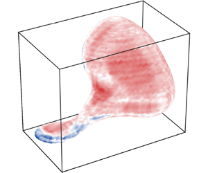
Figure 1(a) shows a schematic of the experimental apparatus in which homogeneous and isotropic turbulence was generated through a jet array (inset). Bubbles were injected to the view volume via a needle connected to a gas line (grey line). A typical breakup process of a bubble is illustrated in figure 2. Four cameras from different angles with back lighting around the view volume were used (figure 1b) to obtain the 3-D Lagrangian trajectories of tracer particles (Tan et al. Reference Tan, Salibindla, Masuk and Ni2020) and also to reconstruct the 3-D geometry of bubbles (Masuk, Salibindla & Ni Reference Masuk, Salibindla and Ni2019a). An example of the reconstructed bubble is shown in the top panel of figure 1(c). To better quantify the local deformation, the bubble interfacial velocity  $u_f$ and mean curvature
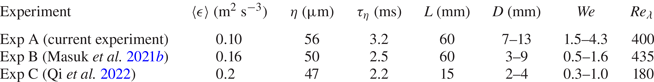
  $\kappa$ are also calculated (as illustrated in figure 1c). More details regarding the experimental set-up and the bubble interfacial velocity and curvature can be found in Appendices A and B. To expand the parameter space further, two supplemental datasets conducted in similar conditions (Masuk et al. Reference Masuk, Salibindla and Ni2021b; Qi et al. Reference Qi, Tan, Corbitt, Urbanik, Salibindla and Ni2022) are also included. Key parameters of all the datasets are summarized in table 1. In total, 385 breakup events (131 for Exp A, 183 for Exp B, and 40 for Exp C) are used for statistics of this work.
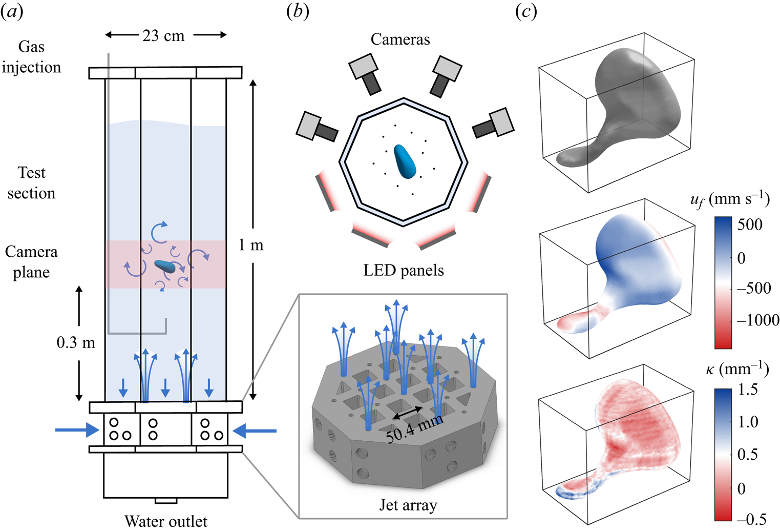
Figure 1. (a) A schematic of the vertical water tank as described in Appendix A. The blue arrows represent the direction of the flow. Inset: a 3-D model of the jet array system for turbulence generation. (b) Top view of the configuration of cameras and LED panels around the octagonal test section. The black dots in the test section represent tracer particles around the bubble. (c) From top to bottom: the 3-D reconstruction of a breaking bubble using the visual hull method; the distribution of the interfacial velocity  $u_f$ for the same bubble; the distribution of the interfacial curvature $\kappa$ for the same bubble.
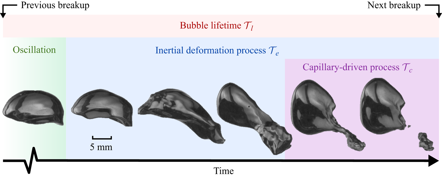
Figure 2. A sequence of snapshots of a breaking bubble with  $D=10$ mm. The green, blue, purple and red shaded area represents the oscillation process, the inertial deformation process, the capillary-driven process and the bubble lifetime, respectively.
Table 1. Summary of parameters and dimensionless numbers of the experimental datasets included in the current work (Exp B and Exp C are the supplementary datasets). Here,  $\eta$, $\tau _\eta$, $L$ and $Re_\lambda$ are the Kolmogorov length scale, Kolmogorov time scale, integral length scale and Taylor-scale Reynolds number, respectively.
2.1. Interfacial curvature
Figure 3(a) shows the probability density functions (PDFs) of the interfacial curvature  $\kappa$ normalized by the bubble radius $D/2$ for bubbles that eventually break in Exp A. Here, $\kappa >0$ and $\kappa <0$ represent convex and concave interfaces, respectively; $t=0$ indicates the instant when the breakup occurs, and $t<0$ represents the moment before the bubble breakup; $\tau _\eta$ is the Kolmogorov time scale. The PDFs for the entire duration, from 10 $\tau _\eta$ prior to the breakup to the breakup moment, follow a similar distribution, although a small difference over time can be observed. The peaks of all the PDFs are located at $\kappa D/2 \approx 0.9$, which is close to the undeformed spherical geometry with the mean curvature exactly at $\kappa D/2=1$. In addition, all the PDFs are positively skewed with a higher probability of finding interfaces with local positive curvatures, i.e. extruded outwards from the gas phase to the ambient liquid. This positive skewness is due potentially to the incompressibility of the inner gas. As part of the bubble interface is compressed by surrounding turbulence (which will be discussed in the following), the rest of the interface tends to extrude outwards. This extrusion might be not uniform but significantly sharp along certain directions with minimum resistance, resulting in $\kappa D/2\gg 1$.
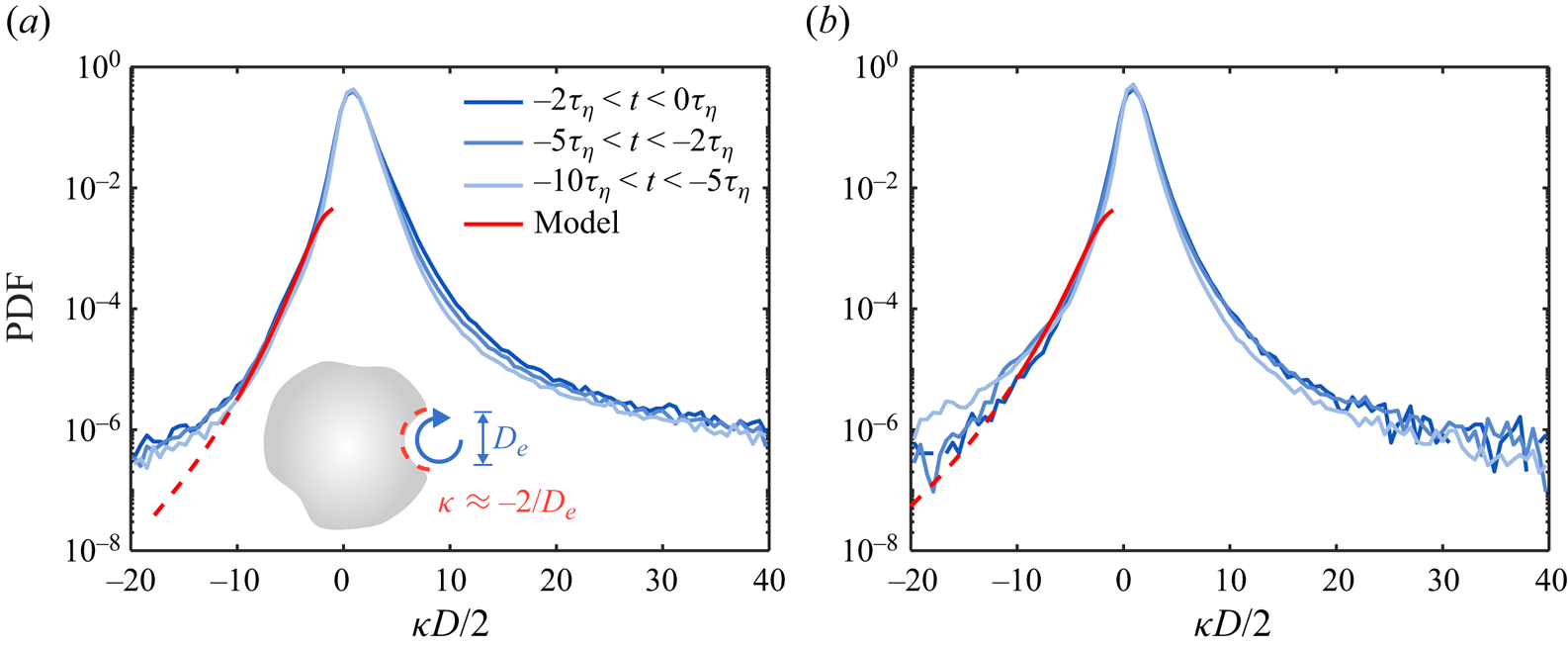
Figure 3. (a) The PDFs of the normalized interfacial curvature  $\kappa D/2$ for all breaking bubbles in Exp A. Blue represents different times before the breakup. The red line represents the prediction based on the model (2.5). The solid part of the red line marks the range of $\kappa$ where the model is valid. (b) The same plots for Exp B.
Note that the negative  $\kappa$ represents the local depression on the bubble interface, which is associated with the increase of local dynamic pressure. If this depression is considered as a result of the collision between the bubble interface and sub-bubble-scale eddies (Luo & Svendsen Reference Luo and Svendsen1996), then the left tail of the PDF can be understood and modelled by accounting for such interactions.
Let us picture a simple scenario in which a bubble with diameter  $D$ encounters an energetic, sub-bubble-scale eddy with size $D_e< D$, as shown in the schematic of figure 3(a). To leading order, the local curvature can be assumed to scale with $1/D_e$, and the other part of the interface remains unchanged given the short interaction time. In order for the eddy to depress the local interface, the inertia of the eddy $\rho u_e^2$ must be comparable with the surface tension induced by the local curvature, i.e. $\sigma /D_e$, where $u_e$ is the velocity of the eddy. This relation leads to $\rho u_e^2>C_1\sigma /D_e$, where $C_1$ is a fitting parameter that will be discussed in detail later. Rearranging this equation leads to the minimum eddy velocity required to deform the interface:
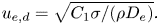 \begin{equation} u_{e,d}=\sqrt{C_1\sigma/(\rho D_e)}. \end{equation}
 The conditional PDF of instantaneous eddy velocity  $u_e$ in turbulence for a given eddy size $D_e$ can be expressed as
 \begin{equation} P(u_e\,|\,D_e)=3\sqrt{2}\,\epsilon_e^{2/3} D_e^{-1/3}\,P(\epsilon_e)/2, \end{equation}
where  $\epsilon _e$ is the local energy dissipation rate at the eddy length scale (Qi et al. Reference Qi, Tan, Corbitt, Urbanik, Salibindla and Ni2022). The distribution of $\epsilon _e$ can be approximated by a log-normal function $P(\epsilon _e)=1/(\epsilon _e\sqrt {2{\rm \pi} \sigma _{\ln \epsilon }^2})\exp {[-(\ln {(\epsilon _e/\langle \epsilon \rangle )}+\sigma _{\ln \epsilon }^2/2)^2/{2\sigma _{\ln \epsilon }^2}]}$, given by the multi-fractal model (Kolmogorov Reference Kolmogorov1962; Meneveau & Sreenivasan Reference Meneveau and Sreenivasan1991). Here, $\sigma _{\ln \epsilon }^2=A+\mu \ln (L/D_e)$ is the variance; $A$ represents a large-scale variability, which is set at $A=0$ for convenience; $\mu \approx 0.25$ is the intermittency exponent; and $L$ is the integral length scale of turbulence.
Given the distribution of the instantaneous eddy velocity (2.2), the PDF of the size of the eddies that are sufficiently strong to depress the bubble interface can be expressed by
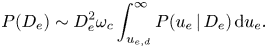 \begin{equation} P(D_e)\sim D_e^2\omega_c \int_{u_{e,d}}^\infty P(u_e\,|\,D_e)\,{\rm d} u_e. \end{equation}
This equation accounts for the interfacial area depressed by the bubble, which scales with  ${\sim }D_e^2$ (as illustrated in figure 3a), and the frequency of the collision between the bubble and an eddy of size $D_e$ (Luo & Svendsen Reference Luo and Svendsen1996; Qi et al. Reference Qi, Tan, Corbitt, Urbanik, Salibindla and Ni2022), which can be estimated using
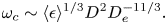 \begin{equation} \omega_c\sim \langle\epsilon\rangle^{1/3}D^2D_e^{-11/3}. \end{equation}
Since the local curvature of the depression can be approximated by  $\kappa \approx -2/D_e$, the PDF of the local negative curvature on the bubble interface can therefore be expressed as
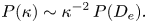 \begin{equation} P(\kappa)\sim\kappa^{-2}\,P(D_e). \end{equation}
 The predicted PDF for  $\kappa <0$ based on (2.5) is shown in figure 3(a) as the red solid curve, with only one fitting parameter $C_1=0.36$ to set the minimum eddy velocity $u_{e,d}$. It is evident that the model prediction agrees with the experimental results but only for a range of $\kappa$ because (2.5) works only for eddies within the inertial range. As a result, the predicted PDF extends only up to $\kappa D/2\approx -10$, corresponding to the eddy size of $D_e\approx 1$ mm, which is close to the lower limit of the inertial range (see Appendix C). In addition, the model can describe only local deformation so it cannot be used to predict the distribution of small curvature that corresponds to large deformation of the bubble size, i.e. $\kappa D/2\approx -1$. Nevertheless, the overall agreement for the scales considered suggests that the bubble local deformation is likely driven by the collision with sub-bubble-scale eddies at least statistically. In figure 3(b), the analysis above is also conducted for Exp B for bubbles with size 3–6 mm, which is around half of the bubble sizes in Exp A. The PDFs follow distributions similar to those in figure 3(a), and a similar good agreement between the model and experiments for the range of scales considered can still be established by setting the fitting parameter $C_1=0.14$ in the model.
Prior to the breakup, as shown in figure 2 by the green shaded area, bubbles experience strong deformation, including frequent stretching and depression, so the variation of curvature could be an indicator of the breakup dynamics. Figure 4(a) shows the time evolution of the averaged standard deviation of the curvature  $\langle \sigma _{\kappa D/2}\rangle$ over all the breaking-bubble trajectories before the breakup occurs for Exp A. It is seen that $\langle \sigma _{\kappa D/2}\rangle$ remains approximately constant until approximately $t=-9\tau _\eta$, when $\langle \sigma _{\kappa D/2}\rangle$ begins to increase gradually, indicating a substantial variation of the interfacial curvature. The associated time scale $\tau _e\approx 9\tau _\eta$, as indicated by the blue shaded area, is then considered as the characteristic time scale of such a turbulence-driven inertial deformation process (Ruth et al. Reference Ruth, Aiyer, Rivière, Perrard and Deike2022) (blue shaded area in figure 2).
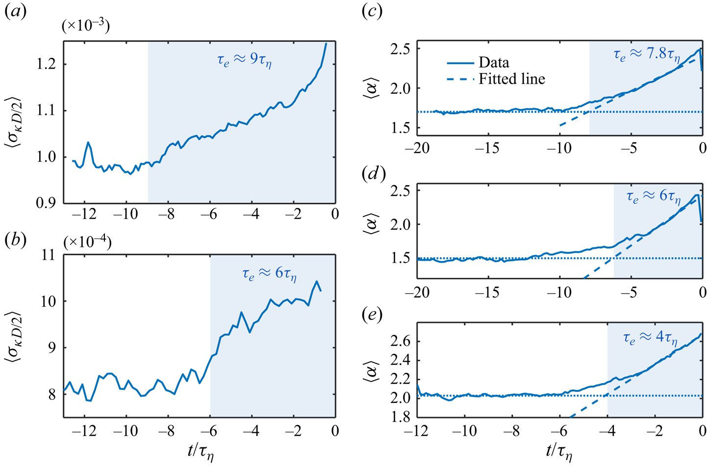
Figure 4. (a) The time evolution of the averaged standard deviation of the curvature  $\langle \sigma _{\kappa D/2}\rangle$ for Exp A. The blue shaded area marks the time scale $\tau _e$. (b) The same plots for Exp B. (c–e) The time evolution of the mean aspect ratio $\langle \alpha \rangle$ (solid lines) of breaking bubbles for Exp A, B and C, respectively. The blue shaded area marks the time scale $\tau _e$.
In addition to the curvature, another quantity that reflects the deformation of bubbles is the aspect ratio  $\alpha$. Figure 4(c) shows the time evolution of the mean aspect ratio $\langle \alpha \rangle$ of all the breaking bubbles for the same dataset prior to the breakup moment. Here, the aspect ratio $\alpha =2r_{maj}/D$ is defined as the ratio between the semi-major axis $r_{maj}$ and the bubble spherical-equivalent radius $D/2$. In figure 4(c), it is evident that $\langle \alpha \rangle$ far from the breakup moment remains almost constant with $\langle \alpha \rangle >1$, suggesting that bubbles experience strong temporal oscillation (as indicated by the green shaded area in figure 2). However, since those fluctuations do not follow the same frequency or phase, averaging the signals over many bubbles results in a nearly constant $\langle \alpha \rangle$. Close to the breakup moment, $\langle \alpha \rangle$ exhibits clear growth, implying that $\alpha$ for all bubbles is likely to increase during this time period. A method is applied to extract this time scale by calculating the intersection between two lines: the dotted line that captures the early plateau, and the dashed line that is fitted over the range of $\langle \alpha \rangle$ from the half-height to the peak, as illustrated in figure 4(c). A time scale approximately $7.8\tau _\eta$ can be then extracted as indicated by the blue shaded area. This time scale is similar to $\tau _e\approx 9\tau _\eta$ obtained from figure 4(a), and is thus considered as the same time scale associated with the bubble inertial deformation driven by turbulence.
The same analysis of  $\langle \sigma _{\kappa D/2}\rangle$ and $\langle \kappa \rangle$ is repeated for Exp B with 3–6 mm bubbles, as shown in figures 4(b,c), respectively. Most of the previous discussion regarding Exp A remains the same here, and a shorter inertial deformation time scale $\tau _e\approx 6\tau _\eta$ can be obtained consistently from the time evolution of both $\langle \sigma _{\kappa D/2}\rangle$ and $\langle \kappa \rangle$. For Exp C, since the bubble is too small so that the reliable reconstruction of the curvature is not possible, $\tau _e$ is determined only based on the time evolution of $\langle \alpha \rangle$ (figure 4e).
2.2. The inertial deformation time scale
Following a procedure similar to that discussed above, the time scale of the inertial deformation, i.e.  $\tau _e$, is extracted and shown in figure 5 for all the datasets. In the case when $\tau _e$ obtained based on the time evolution of $\langle \sigma _{\kappa D/2}\rangle$ and $\langle \kappa \rangle$ is slightly inconsistent (e.g. figures 4a,c), the averaged $\tau _e$ is used.
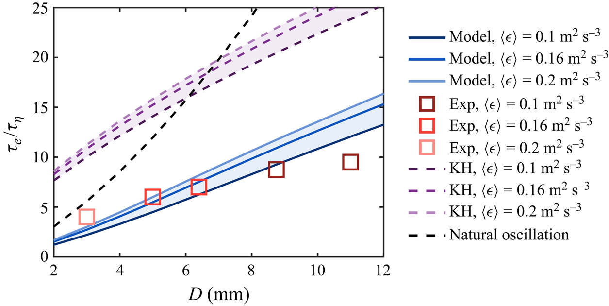
Figure 5. The inertial deformation time scale  $\tau _e$ as a function of the bubble size. Squares represent the experimental data from all the datasets. The solid lines are the predictions based on the model (2.8). The purple dashed lines are the turn-over times of the bubble-sized eddies. The black dashed line represents the second-mode natural oscillation time scale of the bubble.
Given the fact that  $\tau _e$ is driven by surrounding turbulence, two simple approaches are available to model $\tau _e$. The first approach is the Kolmogorov–Hinze (KH) framework (Kolmogorov Reference Kolmogorov1949; Hinze Reference Hinze1955), based on which the time scale of the inertial deformation process $\tau _e$ can be estimated using the turn-over time scale of the bubble-sized eddy, i.e. $\tau _D= D/(\sqrt {C_2}(\langle \epsilon \rangle D)^{1/3})$, which is shown in figure 5 as purple dashed lines for various $\langle \epsilon \rangle$. The other approach is to associate $\tau _e$ with the resonance oscillation of the bubble, which could also lead to breakup (Risso & Fabre Reference Risso and Fabre1998). The time scale of this resonance oscillation is given by $\tau _2=2{\rm \pi} \sqrt {\rho D^3/(96\sigma )}$ (Lamb Reference Lamb1879), which is shown in figure 5 as black dashed lines. In figure 5, it is evident that both approaches overestimate $\tau _e$ compared to the experimental data.
The alternative way to model  $\tau _e$ is by following an approach similar to that in the previous work by Qi et al. (Reference Qi, Tan, Corbitt, Urbanik, Salibindla and Ni2022), in which the sub-bubble-scale eddy contribution to the breakup is incorporated, and the breakup criterion is set by two relationships based on the inertia and time scale of the sub-bubble-scale eddy. Following this work, the minimum requirement of the eddy velocity $u_{e,b}$ (or equivalently, the eddy kinetic energy) to break the bubble can be written as
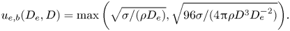 \begin{equation} u_{e,b}(D_e,D)=\max\left(\sqrt{\sigma/(\rho D_e)},\sqrt{96\sigma/(4{\rm \pi} \rho D^3 D_e^{-2})}\right)\!. \end{equation}
Given  $u_{e,b}$, considering the distribution of eddy velocity $P(u_e\,|\,D_e)$ of an eddy (2.2), the probability $P'_b$ for this eddy to break the bubble is expressed following the integration
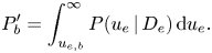 \begin{equation} P'_b=\int_{u_{e,b}}^\infty P(u_e\,|\,D_e)\,{\rm d} u_e. \end{equation}
 In order to estimate the time scale, it is assumed that the time required for a bubble to be broken by an eddy with velocity  $u_e$ is given by $D/(2u_e)$. The factor 2 in the denominator comes from the observation that typically, the formation of the neck involves retraction of the interface simultaneously from both sides. Considering the distribution of eddy velocity $P(u_e\,|\,D_e)$ in (2.2), the breakup probability $P'_b$ from (2.7) and the collision frequency $\omega _c$ (2.4), the expected inertial time scale, i.e. $\tau _e$, can be expressed by
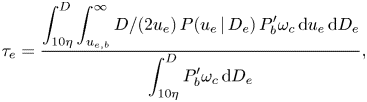 \begin{equation} \tau_e=\frac{\displaystyle\int^D_{10\eta} \int_{u_{e,b}}^\infty D/(2u_e)\,P(u_e\,|\,D_e)\,P_b' \omega_c \,{\rm d} u_e \,{\rm d} D_e}{\displaystyle\int^D_{10\eta}P_b' \omega_c \,{\rm d} D_e}, \end{equation}
where the contribution from all the sub-bubble-scale eddies in the inertial range, from approximately  ${\sim }10\eta$ ( $\eta$ being the Kolmogorov length scale) to the bubble size, are incorporated. Eddies in the dissipation range are not considered here as they have negligible energy to break the bubble, and (2.2) and (2.4) no longer hold. Note that in this model, no free parameter is involved.
It is worth emphasizing the difference between (2.8) and the bubble lifetime model reported in Qi et al. (Reference Qi, Tan, Corbitt, Urbanik, Salibindla and Ni2022). The bubble lifetime model in Qi et al. (Reference Qi, Tan, Corbitt, Urbanik, Salibindla and Ni2022) considers the averaged time required for the bubble to encounter an eddy that eventually leads to a successful breakup, whereas (2.8) is the weighted average of the time between a successful collision event and the final breakup.
The prediction based on (2.8) for various  $\langle \epsilon \rangle$ is shown as blue solid lines in figure 5. Compared to the classical Kolmogorov–Hinze framework, it is evident that the predicted $\tau _e$ agrees better with the experimental data, further emphasizing the role of energetic, sub-bubble-scale eddies in the inertial deformation process. It is noted that the Kolmogorov–Hinze framework (purple lines) could be modified to achieve reasonable agreement with the data by using a different eddy size. Specifically, the eddy size can be assumed to be $\beta D$, where $\beta$ is a coefficient, and the resulting eddy turnover time becomes: $\tau_{\beta D}= \beta D/(\sqrt {C_2}(\langle \epsilon \rangle \beta D)^{1/3})$). To bring the purple lines down to the experimental data in figure 5, it is evident that $\beta$ has to be smaller than 1. This result highlights our point that the inertial deformation time scale could be dominated by the turn-over time scale of a sub-bubble-scale eddy, consistent with the underlying mechanism of (2.8) although only one sub-bubble scale is considered here. Unfortunately, given the range of $We$ covered in this work, it is difficult to conclude which model (modified Kolmogorov–Hinze framework or (2.8)) better predicts the inertial deformation time scale. It is also worth noting that (2.8) slightly over-predicts $\tau _e$ at $D=11$ mm, and it is likely driven by the buoyancy effect. In particular, the Eötvös number $Eo=\rho g D^2/\sigma$ for such bubble size is around $Eo=16.8\gg 1$. This effect likely destabilizes the bubbles and results in an accelerated breakup process, especially for large bubbles with relatively low turbulence intensity.
2.3. Interfacial velocity
In addition to  $\tau _e$, a different time scale can be extracted from the interfacial velocity statistics. Figure 6(a) shows the PDFs of the interfacial velocity $u_f$ for 3–6 mm breaking bubbles over different times in Exp B. Here, $u_f>0$ and $u_f<0$ represent outward and inward interfacial velocity, respectively, from the perspective of bubbles. As a result, $u_f>0$ indicates the interface moving from the gas phase towards the outer liquid phase, and vice versa. In this figure, $u_f$ is normalized by its standard deviation $\sigma _{u_f}'$. It is evident that the PDFs for $t<-2\tau _\eta$ collapse well and follow a similar distribution. However, the PDF at $-2\tau _\eta < t<0$ is slightly off, with a higher left tail and a lower right tail. In addition, all the PDFs clearly deviate from a Gaussian distribution, which is shown in figure 6(a) by the black dashed line. The much higher probability of finding extreme interfacial velocity implies that the interfacial velocity is more intermittent compared to the single-phase fluctuation velocity as shown in figure 6 by the grey solid line. Moreover, the PDFs of $u_f$ are all negatively skewed, indicating that the inward interfacial velocity is substantially stronger compared to the outward. This strong inward interfacial velocity could be linked to the distribution of the interfacial curvature, which shows clear positive skewness (see figure 3). As the majority of the interface is convex with $\kappa D/2\gg 1$, the resulting surface tension pointing inwards from liquid to gas tends to significantly accelerate the contraction of the interface, leading to stronger negative interfacial velocity.
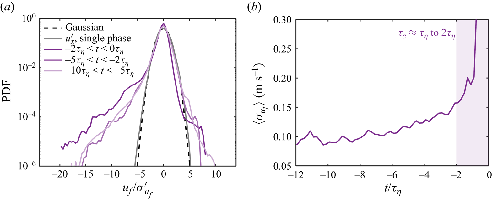
Figure 6. (a) PDFs of the interfacial velocity  $u_f$ for 3–6 mm breaking bubbles in Exp B. Purple solid lines represent the different times before the breakup. The black dashed line marks the Gaussian distribution. The grey solid line shows the PDF of one component of the single-phase fluctuation velocity $u_x^\prime$ normalized by its standard deviation. (b) The time evolution of the averaged standard deviation of the interfacial velocity $\langle \sigma _{u_f}\rangle$. The purple shaded area marks the time scale $\tau _c$.
In addition to the PDFs, the time evolution of the standard deviation of the interfacial velocity, averaged over all the breaking-bubble trajectories  $\langle \sigma _{u_f}\rangle$, is shown in figure 6(b). Here, $\langle \sigma _{u_f}\rangle$ remains almost constant at the beginning, indicating that the distribution of $u_f$ does not experience significant changes. At $t\approx -6\tau _\eta$, approximately one inertial deformation time scale earlier, before the breakup ( $\tau _e\approx 6\tau _\eta$), $\langle \sigma _{u_f}\rangle$ begins to grow. Such growth suggests that the inertial deformation process of the bubble could affect the distribution of the interfacial velocity. Later, at approximately $t\approx -2\tau_\eta$ to $-1\tau _\eta$, another substantial increase of $\langle \sigma _{u_f}\rangle$ is observed. This sudden increase leads to a new time scale $\tau _c\approx \tau_\eta$ to $2\tau _\eta$, as indicated by the purple shaded area in figure 6(b). Note that this time scale $\tau _c$ is significantly shorter than the corresponding inertial deformation time scale ( $\tau _e\approx 6\tau _\eta$), indicating that a distinct physical process occurs right before the breakup.
The mechanism that leads to the sudden increase of  $\langle \sigma _{u_f}\rangle$ is likely linked to the necking process before the neck finally pinches off, as illustrated by the purple shaded area in figure 2. With a sufficient amount of deformation, the neck shrinks rapidly right before the breakup, which is accompanied by a fast and local inward interfacial velocity. This interfacial velocity eventually leads to the sudden increase of $\langle \sigma _{u_f}\rangle$ in figure 6(b), and the rise of the left tail of the PDF in figure 6(a) during $-\tau _c< t<0$.
Based on the discussion above, the time scale  $\tau _c$ of the final pinch-off can be modelled using the capillary time scale that has been discussed before (Villermaux Reference Villermaux2020; Rivière et al. Reference Rivière, Ruth, Mostert, Deike and Perrard2022; Ruth et al. Reference Ruth, Aiyer, Rivière, Perrard and Deike2022). The model of the capillary time scale follows $\tau _c=\rho ^{1/2} \sigma ^{-1/2} \delta ^{3/2}/(2\sqrt {3})$, where $\delta$ is the typical width of the bubble neck that eventually becomes unstable and leads to the rupture of the interface. Here, $\delta$ can be estimated using the size of the smallest daughter bubble resulting from the breakup (Rivière et al. Reference Rivière, Ruth, Mostert, Deike and Perrard2022). In our experiments, the neck width and the daughter bubble size vary from case to case. The mean neck width is estimated of the order of $\delta \sim O(1)$ mm for bubbles with $D\gtrsim 3$ mm. Using $\delta =1$ mm as the neck width leads to an estimation $\tau _c\approx 1.5\tau _\eta$, which is reasonably close to the range of $\tau _c$ measured from the experiment (figure 6b).
2.4. Breakup time scales and separation
Figure 2 illustrates two time scales associated with the breakup process, including the inertial deformation time  $\tau _e$ and the capillary time scale $\tau _c$. In addition, the bubble lifetime $\tau _l$, which is defined as the time interval between two consecutive breakups, is also shown, as indicated by the red shaded area. During this bubble lifetime, bubbles experience complicated deformation and oscillation due to the continuous bombardment by eddies of various sizes (green shaded area), until the event that the bubble encounters intense eddies, leading to strong inertial deformation followed by the neck thinning, which leads ultimately to the breakup.
To further compare the bubble lifetime  $\tau _l$ with the other time scales, the experimental data from previous works are included. Figure 7 shows the measured bubble lifetime $\tau _l$ by Vejražka et al. (Reference Vejražka, Zedníková and Stanovský2018) (red symbols) and Martínez-Bazán et al. (Reference Martínez-Bazán, Montanes and Lasheras1999) (blue symbols) as functions of the Weber number. Here, $\tau _l$ is calculated following $\tau _l=1/g_b$, where $g_b$ is the bubble breakup frequency that can be measured experimentally (Håkansson Reference Håkansson2020). Both datasets show distinct trends. Specifically, Vejražka et al. (Reference Vejražka, Zedníková and Stanovský2018) reported a decrease in bubble lifetime as $We$ increases, while Martínez-Bazán et al. (Reference Martínez-Bazán, Montanes and Lasheras1999) suggested a slightly increasing $\tau _l/\tau _\eta$. This difference in the Weber number dependence marks the decades-long debate on whether the lifetime of bubbles increases or decreases as a function of $We$.
$We$.
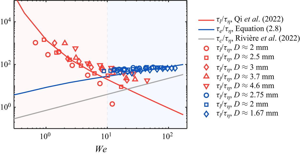
Figure 7. The comparison among different time scales associated with bubble breakup predicted by models, including the bubble lifetime  $\tau _l$ (red solid line), the inertial deformation time scale $\tau _e$ (blue solid line), and the capillary time scale $\tau _c$ (grey solid line), as functions of $We$. The red and blue symbols represent the experimental data of $\tau _l$ by Vejražka et al. (Reference Vejražka, Zedníková and Stanovský2018) and Martínez-Bazán et al. (Reference Martínez-Bazán, Montanes and Lasheras1999), respectively. The red and blue shaded areas mark $We<10$ and $We>10$.
In addition to the experimental results, the solid red line in figure 7 also shows the prediction by a bubble lifetime model (Qi et al. Reference Qi, Tan, Corbitt, Urbanik, Salibindla and Ni2022) for 3 mm bubbles at various  $\langle \epsilon \rangle$. This model already considers the contribution from sub-bubble-scale eddies, i.e. bubble breakups are accelerated by the collisions with sub-bubble-scale energetic eddies with the bubble lifetime dominated by the frequency of those extreme events. The model agrees well with the experimental data for $We\lesssim 10$; however, it decays continuously and underestimates the lifetime for $We\gtrsim 10$. Note that this model does not account for the fact that the lifetime $\tau _l$ cannot drop indefinitely as bubbles still need at least one inertial deformation time scale $\tau _e$ to complete the breakup process. Figure 7 shows the predicted $\tau _e$ by (2.8) for 3 mm bubbles as the blue solid line. The result by (2.8) is consistent with experimental data for $\tau _l$ at the large Weber number limit. Note that both experimental datasets can be explained by considering the maximum between the predicted bubble lifetime (Qi et al. Reference Qi, Tan, Corbitt, Urbanik, Salibindla and Ni2022) and the predicted inertial deformation time scale (2.8), which cross over each other at $We\approx 10$. The agreement suggests that different trends observed in the experiments were the result of the transition of different time scales at play.
This result also highlights the role of the Weber number in determining the time scale separation for breakup in turbulent two-phase flows. For small  $We$, since the majority of collisions between bubbles and surrounding eddies lead only to deformation but not breakup, the lifetime of the bubble is dominated by the long oscillation stage, and the scale separation between the lifetime and the final inertial deformation time scale is significant. Such scale separation depends only on $We$. For large $We$, the two time scales become one, and no scale separation can be observed. This is analogous to the role played by the Reynolds number in controlling the scale separation in single-phase turbulence where the separation between the Kolmogorov scale and integral scale diminishes as $Re$ decreases. The capillary time scale $\tau _c$ (Rivière et al. Reference Rivière, Ruth, Mostert, Deike and Perrard2022) (grey solid line in figure 7), however, remains nearly a small constant regardless of $We$ as it is not affected by surrounding turbulence.
3. Conclusion
The deformation and breakup of bubbles in turbulence involve the interaction between bubbles and eddies of various sizes. Which characteristic time scales control the breakup process is an inherently challenging question to answer, and the framework by Levich (Reference Levich1962) proposed several dominant time scales without specifying the relationships among them. In this work, to examine these time scales, we employed different statistics based on the shape reconstruction of breaking bubbles, including large-scale aspect ratio and small-scale local interfacial deformation through a unique experiment. The distribution of bubble local curvature emphasizes the importance of sub-bubble-scale eddies. Following this hypothesis, a small-eddy collision model to predict the interfacial curvature distribution is proposed and is found to be in good agreement with experimental results. A time scale associated with the inertial deformation of the bubble induced by the collision with sub-bubble-scale eddies and a capillary time scale associated with the neck process are then identified and modelled based on curvature and interfacial velocity statistics. In addition to these time scales, the bubble lifetime is also discussed briefly. It is found that for  $We<10$, the bubble lifetime is dominated by the frequency of energetic sub-bubble-scale eddies that can break the bubble. However, for $We>10$, the majority of sub-bubble-scale eddies are sufficiently energetic, thus this time scale is limited primarily by the inertial deformation time scale. The results highlight how the Weber number controls the separation of time scales in the breakup dynamics, similar to the well-known role of the Reynolds number in determining the scale ratio in single-phase turbulence.
Acknowledgements
We acknowledge Dr Shengze Cai for the useful discussion regarding the interfacial velocity.
Funding
We acknowledge the financial support from the National Science Foundation under the award number CAREER-1905103. This project was also partially supported by the ONR award: N00014-21-1-2083.
Declaration of interests
The authors report no conflict of interest.
Data availability statement
All the data supporting this work are available from the corresponding author upon reasonable request.
Appendix A. Experimental set-up
As illustrated in figure 1(a), a vertical tank was designed to study bubble deformation and breakup in homogeneous and isotropic turbulence (HIT). This vertical tank consists of two main components: an octagonal test section, and an upward-facing jet array system to generate HIT. The figure 1(a) inset shows the jet array, which is designed similarly to the one by Masuk et al. (Reference Masuk, Salibindla, Tan and Ni2019b). The jet array features 21 circular nozzles with separation distance 50.4 mm (as indicated by the black distance arrow). The nozzle diameter is 8 mm, and the nozzles are turned on and off randomly at frequency 0.5 Hz to eliminate any large-scale flows. In this work, water jets were fired at 7 m s $^{-1}$, and 10 out of 21 jets on average were kept on at a time to maximize the turbulence intensity. The jet array introduces only momentum, not mass, into the test section, as the same amount of water injected is also taken back through the 16 square holes.
The octagonal test section is 1 m tall and 23 cm in diameter as an inscribed circle. The wall is made of 25.4 mm thick acrylic sheets for optical access. Four high-speed cameras working at  $1280\times 800$ resolution and 5000 frames per second were used to image the view volume (red shaded area in figure 1a), and four designated LED panels provided diffused light to cast shadows of bubbles and tracer particles onto the camera's imaging plane as shown in figure 1(b). The bubbles were injected directly into the test section via a needle with inner diameter 5 mm, and the air was supplied by a stainless steel gas line (represented by the grey line in figure 1a). The tip of the needle is located at around 6 times the nozzle-to-nozzle separation distance above the jay array, where jets are fully mixed and the generated turbulence becomes homogeneous and isotropic as suggested by Tan et al. (Reference Tan, Xu, Qi and Ni2023). By carefully adjusting the gas flow rate using a syringe pump, a single bubble with diameter ranging from 7 to 13 mm was generated in each run in order to avoid large bubble clusters generated from breakups blocking camera views.
Appendix B. Bubble interfacial velocity and curvature
The octagonal test section as well as the multiple-camera arrangement enabled us to perform 3-D reconstruction of the bubble geometry, from which the bubble trajectory can be then obtained simultaneously. The reconstruction of bubble geometry is performed by adopting the visual hull method (Masuk et al. Reference Masuk, Salibindla and Ni2019a). In this process, the bubble 3-D geometry is reconstructed by calculating the intersection of the cone-like volume extruded from the bubble silhouettes extracted from each camera. Based on the the time-resolved bubble geometry, the interfacial velocity  $\boldsymbol {u}_f$ can be determined following four steps. (i) The bubble geometry is first smoothed by applying a filter with a filter length of around $0.2D$. Applying such a filter inevitably removes the high wavenumber structures on the bubble interface. However, structures below this scale could not be discerned from reconstruction uncertainty anyway. (ii) In order to focus on the interfacial dynamics, the translational motion of the bubble is subtracted based on the bubble trajectories so that the centres of the bubble at different times coincide with one another. (iii) The displacement of the bubble interface on each vertex can be obtained by tracking vertices between two consecutive frames using the nearest neighbour algorithm. By dividing this displacement by the time delay between the two frames, the velocity on each vertex can be calculated. (iv) This velocity is then projected to the normal direction of the interface to acquire the interfacial velocity $\boldsymbol {u}_f$ as the tangential component of the interfacial velocity is not measurable. In addition to $\boldsymbol {u}_f$, the mean curvature $\kappa =(\kappa _1+\kappa _2)/2$ of the bubble interface was also calculated along each bubble trajectory based on the method proposed by Rusinkiewicz (Reference Rusinkiewicz2004). Here, $\kappa _1$ and $\kappa _2$ are the maximum and minimum principal curvatures of the interface, respectively. Figure 1(c) shows examples of the reconstructed bubble geometry, the distribution of $u_f$, and the distribution of $\kappa$ of the same bubble.
Appendix C. Structure function
For the continuous phase, by seeding 60  $\mathrm {\mu }$m tracer particles (with Stokes number $St=0.06$) into the flow, 3-D trajectories of tracers were reconstructed by performing Lagrangian particle tracking using the in-house OpenLPT code (Tan et al. Reference Tan, Salibindla, Masuk and Ni2020). These trajectories were smoothed further by convoluting them with Gaussian kernels (Mordant, Crawford & Bodenschatz Reference Mordant, Crawford and Bodenschatz2004; Ni, Huang & Xia Reference Ni, Huang and Xia2012), from which the tracer velocity was obtained along the trajectory. To better quantify the flow properties, we calculated the second-order structure function for both the longitudinal $D_{LL}(r)$ and transverse $D_{NN}(r)$ components, based on the processed tracer velocity following a similar procedure as in Masuk et al. (Reference Masuk, Salibindla and Ni2021b), where $r$ is the separation distance between a pair of tracer particles. It is noted that based on the Kolmogorov theory (Kolmogorov Reference Kolmogorov1941), the second-order structure function in the inertial range can be estimated using the energy dissipation rate $\langle \epsilon \rangle$, i.e. $D_{LL}=C_2(\langle \epsilon \rangle r)^{2/3}$ and $D_{NN}=(4/3)C_2(\langle \epsilon \rangle r)^{2/3}$, where $C_2\approx 2$ is the Kolmogorov constant. These relations provide a way to estimate $\langle \epsilon \rangle$ following $\langle \epsilon \rangle =(D_{LL}/C_2)^{3/2}/r$ and $\langle \epsilon \rangle =[3D_{NN}/(4C_2)]^{3/2}/r$, as shown in figure 8. It is evident that both $D_{LL}$ and $D_{NN}$ seem to collapse well in the inertial range where the plateau is shown. Within the inertial range, $\langle \epsilon \rangle$ can be estimated by extracting the magnitude of the plateau, i.e. $\langle \epsilon \rangle \approx 0.1$ m $^2$ s $^{-3}$. Note that $\langle \epsilon \rangle$ values estimated based on both $D_{LL}$ and $D_{NN}$ are consistent with each other, suggesting that the flow is close to homogeneous and isotropic.
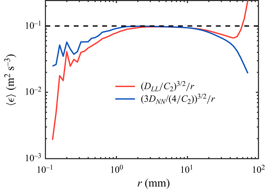
Figure 8. Estimated energy dissipation rate  $\langle \epsilon \rangle$ based on the longitudinal (red) and transverse (blue) second-order structure function. The dashed line represents $\langle \epsilon \rangle =0.1$ m $^2\,$s $^{-3}$.
Based on  $\langle \epsilon \rangle$ obtained from figure 8, the Kolmogorov length scale $\eta$ and Kolmogorov time scale $\tau _\eta$ can be estimated by following $\eta =(\nu ^3/\langle \epsilon \rangle )^{1/4}=56$ $\mathrm {\mu }$m and $\tau _\eta =(\nu /\langle \epsilon \rangle )^{1/2}=3.2$ ms, where $\nu$ is the kinematic viscosity of the flow. Given the range of bubble sizes $D$ generated, the Weber number following $We=\rho C_2 (\langle \epsilon \rangle D)^{2/3} D /\sigma$ ranges from $1.5$ to $4.3$, indicating that turbulence is sufficiently strong to drive the deformation and breakup of bubbles in our system. Here, $\rho$ is the density of the continuous phase, and $\sigma$ is the surface tension coefficient.


 Open access