


Introduction
Electron energy loss spectroscopy (EELS) data acquired at sufficiently large scattering angles display a broad Compton peak, which is a two-dimensional “slice” at constant momentum through the three-dimensional Bethe surface (Inokuti, Reference Inokuti1971; Schattschneider & Exner, Reference Schattschneider and Exner1995; Egerton, Reference Egerton2011). The Compton peak is due to scattering of the incident electron with an atomic electron in the solid. In the so-called impulse approximation, where the energy transfer is much larger than the binding energy of the atomic electron, the scattering can be treated independently of the neighboring atomic electrons and nuclei, i.e. the scattering is strictly a two-body collision event (Cooper et al., Reference Cooper, Mijnarends, Shiotani, Sakai and Bansil2004). The Compton signal then gives information on the momentum density of states of the atomic electrons projected along the scattering vector (Cooper et al., Reference Cooper, Mijnarends, Shiotani, Sakai and Bansil2004). Significantly, the extracted electronic structure corresponds to the ground state of the solid, and is free of excited state artifacts, unlike, for example, the near-edge fine structure in core loss edges, which can be distorted by the core hole (Mizoguchi et al., Reference Mizoguchi, Olovsson, Ikeno and Tanaka2010; Mendis & Ramasse, Reference Mendis and Ramasse2021).
A limited number of electron Compton measurements have been performed, such as on carbon-based materials (Williams et al., Reference Williams, Sparrow and Egerton1984; Exner et al., Reference Exner, Schattschneider and McCarthy1996; Feng et al., Reference Feng, Löffler, Eder, Su, Meyer and Schattschneider2013, Reference Feng, Zhang, Sakurai, Wang, Li and Hu2019; Talmantaite et al., Reference Talmantaite, Hunt and Mendis2020) and silicon (Jonas & Schattschneider, Reference Jonas and Schattschneider1993; Exner & Schattschneider, Reference Exner and Schattschneider1996). Although the Compton intensity is comparable to phonon scattering in low atomic number solids (Eaglesham & Berger, Reference Eaglesham and Berger1994), its analysis using EELS has not been as widespread as X-ray and γ-ray photon-based methods. This is partly due to electron beam damage of the specimen during the time it takes to acquire the relatively weak Compton signal. However, this can now largely be mitigated by advances in instrumentation, such as EELS spectrometers with direct electron detection capability (Cheng et al., Reference Cheng, Pofelski, Longo, Twesten, Zhu and Botton2020; Plotkin-Swing et al., Reference Plotkin-Swing, Corbin, De Carlo, Dellby, Hoermann, Hoffman, Lovejoy, Meyer, Mittelberger, Pantelic, Piazza and Krivanek2020) and/or low-kV microscopy performed below the knock-on damage threshold for specimens undergoing sputter damage (Krivanek et al., Reference Krivanek, Dellby, Murfitt, Chisholm, Pennycook, Suenaga and Nicolosi2010). Talmantaite et al. (Reference Talmantaite, Hunt and Mendis2020) have also shown that accurate Compton data can be acquired from only a subset of the atomic electrons, e.g. the lower binding energy valence and semi-core electrons. This has the advantage that the acquisition time is shorter compared to the total Compton signal due to all electrons. Furthermore, post-processing of the data to numerically remove the core electron contribution is not required (Cooper, Reference Cooper, Mijnarends, Shiotani, Sakai and Bansil2004). The measured Compton peak can therefore be directly interpreted in terms of the important valence electrons that govern solid-state bonding.
While there are strategies to mitigate specimen damage, multiple scattering artifacts arguably present a more fundamental limitation. Here, Bragg diffraction in a crystalline specimen and thermal diffuse scattering (TDS) can act as additional sources of Compton scattering that occur at different momentum transfers to the unscattered beam (Williams et al., Reference Williams, Uppal and Brydson1987). The measured Compton profile will therefore be different to that obtained from a thin specimen undergoing kinematical scattering, where the unscattered beam is the dominant feature in the diffraction pattern. In Compton analysis of crystalline specimens, Bragg diffraction is often unavoidable, especially if the Compton peak is acquired along low index crystallographic scattering vectors. For example, anisotropy studies in electron bonding require measuring the Compton signal along different scattering vectors, which are often low index (Cooper et al., Reference Cooper, Mijnarends, Shiotani, Sakai and Bansil2004). For EELS to rival photon-based Compton analysis, multiple scattering artifacts must be corrected. Although multiple scattering can be minimized by using focussed ion-beam (FIB) microscopy to prepare highquality thin specimens (Schaffer et al., Reference Schaffer, Schaffer and Ramasse2012), there is a limit to how thin specimens can be made before surface effects (i.e., amorphous and surface oxide layers) begin to dominate. Therefore, experimental and data processing techniques to reduce multiple scattering artifacts are desirable.
In this work a multislice (Kirkland, Reference Kirkland2010) technique is used to simulate electron Compton profiles for a given electron momentum density of states under dynamical diffraction conditions. A similar approach has previously been used by Williams et al. (Reference Williams, Uppal and Brydson1987), where the multislice simulated Bragg diffracted beams at a given specimen depth were treated as additional sources of Compton scattering. However, the work of Williams et al. (Reference Williams, Uppal and Brydson1987) did not take into account dynamical scattering of the primary electrons as they exited the specimen following the Compton energy loss event. This is a similar problem to calculating electron backscatter diffraction (EBSD) patterns, where the electron trajectories following a high angle backscattering event must be determined. In EBSD, the problem is simplified by invoking the principle of reciprocity (Winkelmann et al., Reference Winkelmann, Trager-Cowan, Sweeney, Day and Parbrook2007, Winkelmann Reference Winkelmann2010), i.e. the trajectory of the far-field exit wave electron is reversed to determine the internal scattering processes of interest within the solid. The principle of reciprocity has also been used to explain Kikuchi band contrast (Kainuma, Reference Kainuma1955), as well as core-loss EELS signals (Rusz et al., Reference Rusz, Rubino and Schattschneider2007). Based on this principle, our simulations employ two multislice calculations: the conventional forward multislice of Williams et al. (Reference Williams, Uppal and Brydson1987) to determine Bragg sources of Compton scattering, and a reverse multislice, based on the principle of reciprocity, to model dynamical diffraction following the Compton event. Simulations compare favorably with experimental results obtained for a silicon test specimen, and indicate the importance of the incident electron beam and EELS detection geometries on the measured Compton profile. By optimizing the EELS detection geometry, it is possible to minimize Compton artifacts, while maintaining the required specimen diffraction conditions. Furthermore, an inversion method for extracting the projected momentum density of states from a Compton profile acquired from a diffracting specimen is also proposed. This is similar in principle to removal of elastic scattering from EELS core loss edges (Neish et al., Reference Neish, Lugg, Findlay, Haruta, Kimoto and Allen2013). These advances help improve the robustness of electron Compton analysis of crystalline specimens. The simulation method is discussed in more detail in the “Materials and Methods” section, while experimental data and inversion of dynamical Compton results are presented in the “Results and Discussion” section.
Materials and Methods
Experimental Procedure
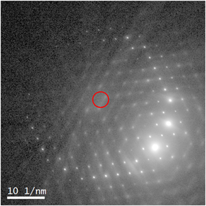
An argon ion-polished silicon 〈110〉 single crystal specimen was examined at 200 kV in a JEOL 2100F field emission gun transmission electron microscope (TEM). Compton spectra were acquired using a Gatan GIF Tridiem EELS spectrometer, under two diffraction conditions: (i) kinematical, where Bragg scattering was minimal, and (ii) dynamical, with the 004 reflection in the Bragg orientation. For the former the sample was first tilted 103.4 mrad away from the 〈110〉 zone axis, to avoid strong diffraction conditions. Using the microscope beam tilt coils the parallel electron beam was then tilted by 48.6 mrad, taking care to avoid excitation of Bragg reflections as much as possible. A 5.3 mrad radius objective aperture was inserted along the optic axis and the EELS Compton signal acquired in centered dark-field image mode with 0.5 eV/channel dispersion (this will be referred to as the “off-axis” spectrum). The high intensity low energy loss region and low intensity Compton peak were acquired separately, and subsequently spliced to give a complete EELS spectrum with good signal-to-noise ratio at all energy losses. An EELS spectrum was also acquired with the electron beam parallel to the optic axis (the “on-axis” spectrum), which contained all the usual features [i.e. zero loss peak (ZLP), plasmons, core loss edges etc.] apart from the Compton peak. The on-axis spectrum is used for subtracting the background under the Compton profile. By using the wedge shape of the specimen “on” and “off-axis” EELS spectra could be acquired at different specimen thicknesses. The diffraction pattern for one such kinematical Compton peak measurement is shown in Figures 1a (linear intensity scale) and 1b (log scale). For the dynamical Compton spectrum the sample was first tilted to the 〈110〉 zone axis. Using the microscope beam tilt coils the parallel electron beam was then tilted 48.8 mrad away from the zone axis, such that the 004 reflection was in the Bragg orientation. “On” and “off-axis” EELS spectra were acquired at different specimen thicknesses. An example diffraction pattern for the dynamical Compton measurement is shown in Figure 1c (linear intensity scale) and 1d (log scale).

Fig. 1. Example diffraction pattern for the kinematical Compton measurement shown in both (a) linear and (b) logarithmic intensity scale. The red circle denotes the position and size of the objective aperture used for electron Compton measurement in centred dark-field mode. (c,d) An example diffraction pattern for the dynamical Compton measurement in linear and logarithmic intensity scales respectively. The 004 reflection is in the Bragg orientation and the red circle denotes the objective aperture.
Simulation Method
The multislice simulation follows the experimental setup for the dynamical Compton measurements and is illustrated schematically in Figure 2a. The sample is 〈110〉 Si. A tilted plane wave, Ψinc, is incident on the specimen entrance surface. Ψinc is multislice propagated within the specimen using the method of Ishizuka (Reference Ishizuka1982) for tilted beams. To avoid aliasing artifacts the beam tilt was rounded to the nearest reciprocal space pixel for the multislice supercell (Barthel et al., Reference Barthel, Cattaneo, Mendis, Findlay and Allen2020). At depth “d” a Compton scattering event at point “P” is assumed to take place. Compton scattering takes place in many directions, and the primary electrons can undergo further elastic and, to a lesser extent, inelastic scattering before they exit the specimen. However, only those primary electrons that are scattered in the direction of the EELS aperture will be detected. In our case this would be the wavefunction Ψexit along the electron-optic axis (Fig. 2a). By reversing the direction of Ψexit, and performing a reverse multislice calculation, it is possible to reconstruct the Compton electron wavefunction at depth “d” that is measured by EELS. In our measurements the energy loss due to Compton scattering is small  $( {\rm \lesssim }1\;{\rm keV})$, so that the reverse multislice calculation is also performed at the primary beam energy. In fact, both the forward and reverse multislice calculations assume elastic scattering only, although inelastic scattering events, such as plasmons (Mendis, Reference Mendis2019, Reference Mendis2020), can also be included at some extra computational cost.
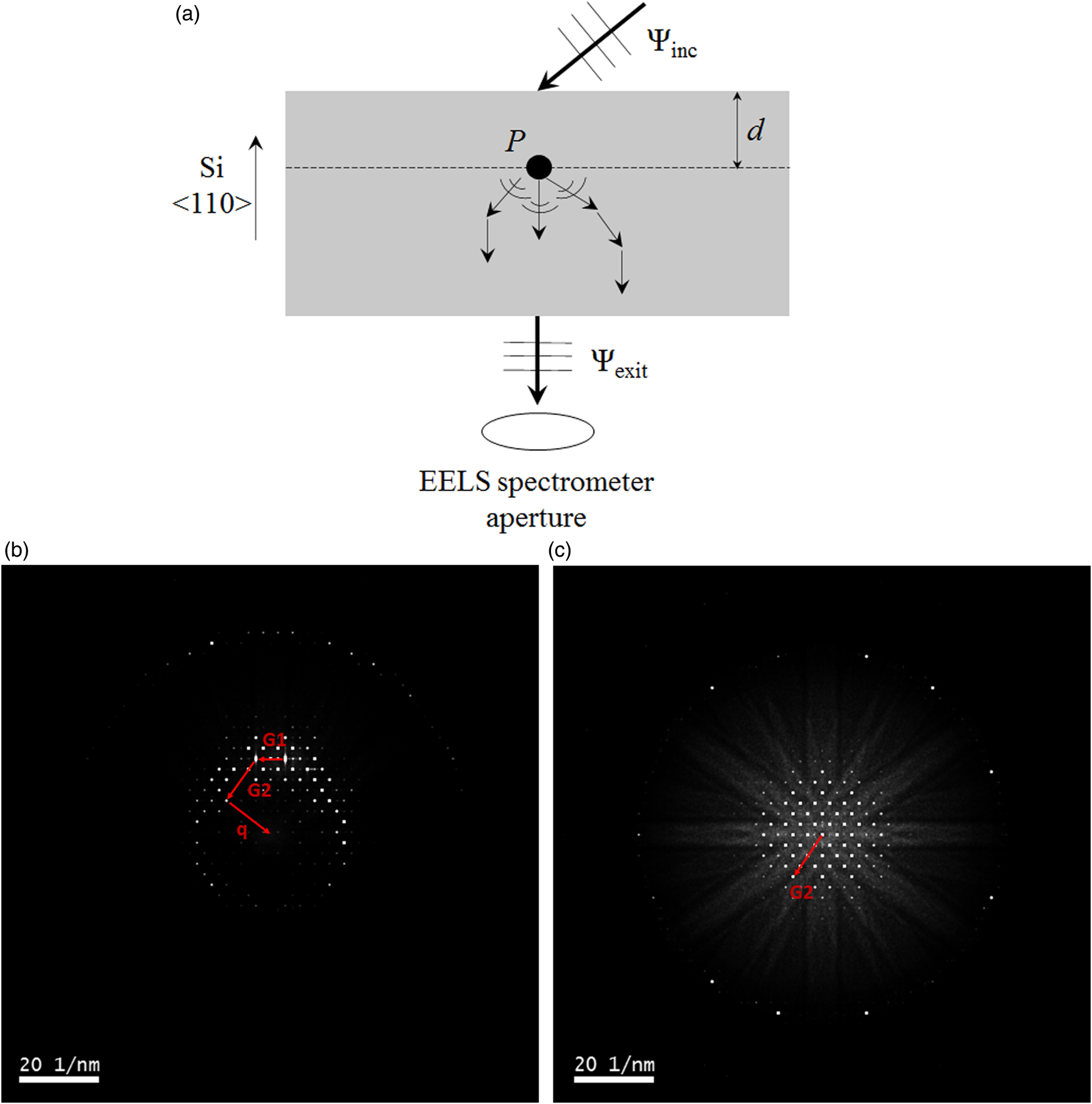
Fig. 2. (a) Schematic illustrating a Compton scattering event at position “P” within a Si 〈110〉 specimen. The incident electron undergoes further scattering after the Compton event, but only those electrons that exit the specimen in the direction of the EELS aperture will be detected. The forward and reverse multislice simulated diffraction patterns (50 frozen phonon configurations) in the middle of a 70 nm thick, Si 〈110〉 specimen are shown in (b,c) respectively. The incident electron beam is tilted 48.8 mrad to the optic axis and is in the 004 Bragg orientation. The EELS spectrometer aperture is along the Si 〈110〉, or equivalently, optic axis. See text for a discussion on G1, G2, and q scattering vectors.
If the projected electron momentum density of states for the solid, J(pz), is known, the electron Compton profile under dynamical diffraction conditions can be simulated as follows. The forward multislice electron wavefunction at depth “d” is Fourier transformed to reveal the Compton scattering sources in reciprocal space. In principle, each point in the diffraction pattern can act as a Compton source, but here we limit our attention to the unscattered and Bragg diffracted beams, which have higher intensity. An example Bragg diffracted beam G1 in the forward multislice diffraction pattern is shown in Figure 2b. Next the reverse multislice electron wavefunction at depth “d” is Fourier transformed to reveal the permissible scattering vectors for the Compton scattered electron before being collected by the EELS aperture. All points in the diffraction pattern represent potential scattering vectors, although for computational convenience only the high intensity unscattered and Bragg diffracted beams are considered. An example Bragg reciprocal vector G2 in the reverse multislice diffraction pattern is shown in Figure 2c and superimposed in Figure 2b. The Compton scattering vector q, must connect (G1 + G2) to the EELS spectrometer aperture, here assumed to be a point at the origin (Fig. 2b). Note that the EELS collection angle is effectively limited by the small objective aperture (5.3 mrad), which justifies the assumption of a point detector. The Compton scattered intensity is proportional to [I(G1)I(G2)]/q 4, where I(G1) and I(G2) are the intensities of the diffracted beams G1 and G2 as calculated by the forward and reverse multislice simulations at specimen depth d for Compton scattering. I(G1) is a function of the incident beam illumination, while I(G2) depends on the EELS collection geometry. The q 4 factor is derived from the Compton scattering cross-section (Williams et al., Reference Williams, Uppal and Brydson1987; Schattschneider et al., Reference Schattschneider, Pongratz and Hohenegger1990). The Compton profile shape is given by J(pz), where pz is the magnitude along the scattering vector q. pz can be converted to energy loss, ΔE, according to (Talmantaite et al. Reference Talmantaite, Hunt and Mendis2020):
 $$\Delta E( {\,p_z} ) = \Delta E_p + \delta E( {\,p_z} ), $$
 $$\Delta E_p = 2{\rm si}{\rm n}^2\displaystyle{\varphi \over 2}\left({2T + \displaystyle{{T^2} \over {m_0c^2}}} \right),$$
 $$\delta E( {\,p_z} ) = {-}p_z\sqrt {\displaystyle{{2\Delta E_p} \over {m_0}}}, $$
where T is the primary electron energy, m 0c 2 is the rest mass energy of the electron, ΔE p is the Compton peak energy at pz = 0, and φ is the Compton scattering angle, which, at small angles, is related to the magnitude of the primary electron momentum p inc by  $\vert {\bf q} \vert = 2p_{{\rm inc}}{\rm sin}( {\varphi /2} )$. The above equations are derived within the impulse approximation. The Compton profile calculated from J(pz) and equations (1a)–(1c) must be normalized to the total number of electrons undergoing Compton scattering, i.e. 12 electrons per atom, for Compton energy losses between Si L- and K-edges. Normalization can effectively be achieved by dividing the Compton intensity by $\sqrt {\Delta E_p}$. This follows from equation (1c) which links momentum pz to energy loss; the energy loss axis is “stretched” by an amount proportional to $\sqrt {\Delta E_p}$, so that the intensity axis must be divided by the same term to keep the area under the Compton profile constant. The electron Compton spectrum I(E) is then:
 $$I( E ) = \mathop \sum \limits_{d, {\bf G}_1, {\bf G}_2, p_z} \displaystyle{{I( {{\bf G}_1} ) I( {{\bf G}_2} ) } \over {q^4}}\left[{\displaystyle{{J( {\,p_z} ) } \over {\sqrt {\Delta E_p} }}} \right]\delta ( {E-\Delta E( {\,p_z} ) } ), $$
where the Dirac delta function is equal to unity when the energy loss E is equal to ΔE(p z), but zero otherwise. The summation over d calculates Compton scattering contributions at different specimen depths.
The Si 〈110〉 supercell for multislice simulation had lateral dimensions 7a o × 5√2a o, where a o is the unit cell lattice parameter. The bandwidth limited, maximum scattering angle is 111 mrad, sufficient for the large beam tilts (48.8 mrad) used in the forward multislice calculation. The supercell thickness was 70 nm, consistent with the experimental specimen thickness measured using EELS. The supercell was divided into thin slices, with thickness a o/√8 or 1.9 Å. Kirkland's (Reference Kirkland2010) atom scattering factors were used to calculate the projected potential for a given slice, and 50 frozen phonon configurations were sampled to reproduce thermal diffuse scattering (Loane et al., Reference Loane, Xu and Silcox1991). Atomic motions were uncorrelated and were based on an rms displacement value of 0.078 Å for silicon (Kirkland, Reference Kirkland2010).
J(pz) for silicon was extracted from the kinematical Compton measurement (see Results and Discussion section). The simulations do not take into account any anisotropy in J(pz), although this introduces only a minor error (~1%; Cooper et al., Reference Cooper, Mijnarends, Shiotani, Sakai and Bansil2004). In principle, the anisotropy can easily be incorporated if J(pz) has been parameterized in lattice harmonics (Jonas & Schattschneider, Reference Jonas and Schattschneider1993). Compton profiles for each slice along the specimen thickness direction was calculated as described previously and summed to give the final result. The symmetry of the Si 〈110〉 diffraction pattern was used to locate Bragg peaks within a 3 Å−1 radius from the reciprocal space origin. Nearly 300 zero order Laue zone (ZOLZ) reflections are included within this search radius. Furthermore, the forward multislice diffraction pattern also included a search for reflections in the higher order Laue zone (HOLZ) ring (Fig. 2b). Care must be taken to avoid “beating” or Moiré effects due to the discrete sampling of the Compton spectrum and pz values [equation (1c)]. For example, in most cases there was a one-to-one correspondence between pz and Compton energy channel, although the mismatch in sampling between the two caused some energy channels to have contributions from two neighboring pz-values, resulting in a near doubling in the intensity of that channel. This was avoided by ensuring that each energy channel had only one pz contribution (the precise pz value does not matter, so long as the sampling is fine enough). The minimum value of ΔE p [equation (1b)] was set to 200 eV (see the discussion on Fig. 3c), and ΔE p values below this threshold were ignored.

Fig. 3. (a) Kinematical Compton spectra acquired at different (t/λ) values. The integrated intensity of the Si L-edge has been normalized for a direct comparison. (b) The corresponding low-loss region of the EELS spectra, with the intensity of the ZLP normalized. (c) The extracted kinematical Compton profile, with the underlying background subtracted using two different methods, namely constant (t/λ) and constant plasmon to ZLP ratio. The arrow indicates the residual Si L-edge intensity due to errors in the background subtraction. (d) The projected momentum density of states J(pz) extracted from the high energy side of the kinematical Compton profile. Also shown for comparison are the γ-ray results of Reed & Eisenberger (Reference Reed and Eisenberger1972).
A limitation of the simulation method is that the mixed dynamic form factor (MDFF), due to interference effects, is not taken into account (Exner & Schattschneider, Reference Exner and Schattschneider1996). The MDFF contribution is zero at the Bragg orientation for small Ewald spheres, where the outgoing Compton scattered electron can effectively be treated as a plane wave. In our case, the incident electron beam is at the Bragg orientation for the 004 reflection, but the larger Ewald sphere at 200 kV means that the Compton scattered electron is more accurately described as a Bloch wave within the crystal. The role of interference effects on our measurements are therefore unknown.
Results and Discussion
Kinematical Compton Scattering
Figure 3a shows kinematical Compton spectra acquired from sample regions of varying thicknesses. The graphs have been normalized to the integrated intensity of the Si L-edge and the thickness (t) is expressed as a ratio of the inelastic mean free path (λ). The calculated Compton peak energy [equation (1b)] is 565 eV, less than the measured value of ~590 eV. The underestimation in the theoretical value is attributed to the additional 1/q 4 term in the Compton scattering cross-section (Su et al., Reference Su, Schattschneider and Zeitler1994). At large scattering angles, the Si L-edge is suppressed due to Compton scattering (Inokuti, Reference Inokuti1971). The characteristic scattering angle for Si L core loss excitation is only 0.25 mrad (Egerton, Reference Egerton2011) and is peaked in the direction of the incident electron beam. The appearance of a Si L-edge in the “off-axis” spectrum must therefore be due to elastic and thermal diffuse scattering altering the angular distribution of the core loss electrons (Su et al., Reference Su, Jonas and Schattschneider1992; Talmantaite et al., Reference Talmantaite, Hunt and Mendis2020). The peak-to-background ratio of the Compton profile decreases rapidly with specimen thickness, although the shape and peak position shows no significant change (Fig. 3a). Consider the effect of multiple inelastic scattering. The corresponding EELS low loss region is shown in Figure 3b. Although multiple plasmon peaks are excited with increasing specimen thickness, the width of a plasmon peak is significantly smaller than the Compton profile (i.e. 5.5 eV versus 417 eV full-width-at-half-maximum). Convolution of the broad Compton signal with a narrow plasmon peak during multiple inelastic scattering should therefore have very little effect on the former, provided the specimen is reasonably thin. Furthermore, the observed changes to the Si L-edge with increasing specimen thickness are comparatively minor (Fig. 3a). This suggests that multiple plasmon scattering is not responsible for the peak-to-background ratio. Instead other factors, such as TDS, may be responsible. For example, TDS in the thicker specimens could decrease the (high scattering angle) Compton signal from the unscattered beam being collected by the finite EELS aperture, while also increasing the measured (low scattering angle) Si L-signal. Irrespective of the exact mechanism, the results indicate the importance of collecting Compton spectra from thin specimens, even under kinematical diffraction conditions.
Subtracting the background under the Compton profile is challenging due to the Si L-edge and the need to extrapolate out to very large energy losses. Su et al. (Reference Su, Jonas and Schattschneider1992) used a numerical method based on multiple elastic–inelastic scattering to model the background, but here the collection of the “on-axis” EELS spectrum provides an alternative empirical route for background subtraction. The “on-axis” spectrum is acquired from the same specimen area and contains the Si L-edge but no Compton peak. A simple subtraction of the “on-axis” spectrum from the “off-axis” spectrum is however not sufficient, since the t/λ for the two measurements will be different. This is because the electron beam in the “off-axis” spectrum is highly tilted, so that the effective specimen thickness is larger. The inelastic mean free path λ will also be slightly different, since the energy loss mechanisms for the “on-axis” spectrum do not include Compton scattering. To approximately correct these errors, the “on” and “off-axis” spectra acquired at different specimen thicknesses were interpolated to a common (t/λ) value of 0.5 before subtraction [spline interpolation of the intensity was applied to each energy loss channel in the raw data set, which consisted of EELS spectra acquired at different (t/λ) values]. The result is shown in Figure 3c and indicates that the Si L-edge has not been fully subtracted, especially at the edge onset region. The residual Si L-signal is likely due to slight changes in the edge shape with multiple inelastic scattering. In particular, Figure 3a shows that plasmon excitation transfers some of the Si L-edge onset intensity to higher energy loss. Therefore, an alternative method would be to interpolate the “on” and “off-axis” spectra to a common plasmon to ZLP intensity ratio before subtraction, since then the multiple inelastic scattering would be similar (the intensity of the first plasmon peak is used to calculate the ratio). The result, superimposed in Figure 3c, indicates that the Si L-edge has been satisfactorily removed. Strictly speaking, this method of background subtraction is still only approximate, due to the specimen diffraction conditions being different for the “on” and “off-axis” spectra, and the role this has on the angular distribution of the inelastically scattered electrons (Su et al., Reference Su, Jonas and Schattschneider1992). Nevertheless, for the experimental conditions in this work background subtraction via the plasmon to ZLP ratio method produced reasonable results, and is therefore employed throughout.
The background-subtracted, kinematical Compton profile shows several interesting features. First, there is an abrupt change in gradient at ~200 eV. This is only twice the energy of the Si L-edge onset, which suggests that the L-shell electrons may cease to undergo Compton scattering at these low energy losses. There is also a smaller change in gradient at ~384 and ~840 eV, which likely represents the transition between the M-shell valence electrons that give rise to the Compton peak and L-shell semi-core states that form the broader, underlying background. The Fermi momentum calculated using free electron theory (Kittel, Reference Kittel2005) has magnitude 0.95 atomic units (a.u.), while equation (1c) predicts values of 1.14 and 1.40 a.u. for energy losses 384 and 840 eV respectively (the different momentum values is due to a slight asymmetry in the Compton profile; Fig. 3c). Although the high energy side of the Compton profile may therefore appear to be less accurate, it is nevertheless used to extract J(pz), since there is no abrupt cut-off in Compton signal (cf. the low energy side at 200 eV). The J(pz) is shown in Figure 3d, with the area under the curve and its mirror reflection normalized to 12 electrons. The normalization is only approximate, since the curve has not fully decreased to zero for the largest measured pz. Also superimposed is the J(pz) data obtained from γ-ray scattering, along with the M-shell valence and 1s 22s 22p 6 core electron contributions, the latter estimated theoretically (Reed & Eisenberger, Reference Reed and Eisenberger1972). The electron J(pz) has larger values, due to the incorrect normalization. However, the width is also greater than the γ-ray result, suggesting a discrepancy between the two measurements. Jonas and Schattschneider observed better agreement between their electron Compton measurements and the same γ-ray result (see Fig. 6a of Jonas & Schattschneider, Reference Jonas and Schattschneider1993). The Compton signal in Jonas & Schattschneider (Reference Jonas and Schattschneider1993) was however acquired at a much higher peak energy of ~1 keV and therefore higher scattering angle, which may have resulted in a more favorable (i.e. closer to kinematical) specimen diffraction condition.
Dynamical Compton Scattering and Its Inversion
Figure 4a shows dynamical Compton spectra acquired at different specimen thicknesses with the 004 reflection in the Bragg orientation. The scattering angle for the kinematical and dynamical measurements are similar (49 mrad), and therefore the Compton peak energy should be approximately equal [equation (1b)]. Furthermore, due to the symmetry of the diamond cubic silicon unit cell, the Compton scattering vectors for the 004 and unscattered beams are both crystallographically equivalent (Jonas & Schattschneider, Reference Jonas and Schattschneider1993). Therefore, any J(pz) anisotropy should also have no effect on the measurement. Despite this the dynamical Compton profile is very different to the kinematical result, and shows a large peak shift to lower energy values, consistent with previous simulations (Williams et al., Reference Williams, Uppal and Brydson1987). The background-subtracted dynamical Compton signal is shown in Figure 4b; the asymmetry of the curve is now more pronounced, with a long “tail” on the high energy side. The multislice simulated result is also superimposed in Figure 4b, with the maximum intensity of the two curves normalized. The simulation reproduces the Compton peak energy satisfactorily, but under/overestimates the high and low energy sides respectively. This could be due to several factors which are simulation related, such as ignoring interference effects (Exner & Schattschneider, Reference Exner and Schattschneider1996) and plasmon energy losses in multislice, as well as systematic experimental errors in the kinematical J(pz) profile.

Fig. 4. (a) Dynamical Compton spectra acquired at different (t/λ) values with the 004 reflection in the Bragg orientation. The integrated intensity of the Si L-edge has been normalized for a direct comparison. (b) The background subtracted, experimental dynamical Compton profile and its comparison with the multislice simulation (50 frozen phonon configurations). The maximum intensity of the two curves have been normalized. (c) The [I(G1)I(G2)]/q 4 intensity contributions at different Compton scattering angles obtained from the multislice simulation. (d) Electron Compton spectrum acquired with the silicon specimen tilted away from the 〈110〉 zone axis and incident beam in the 004 Bragg orientation.
The multislice simulation provides information on the Compton signal “intensity” as a function of scattering angle (Fig. 4c). Here “intensity” refers to the sum of [I(G1)I(G2)]/q 4 proportionality terms at different specimen depths (see Section “Simulation Method”). The dominant contribution is from the unscattered beam, but there are also significant contributions from lower angles which cause the overall Compton peak to shift to lower energies. The 35 and 41 mrad scattering angles, which have the second and third highest contributions to the Compton signal (Fig. 4c), lie close to the trace of the Ewald sphere in the ZOLZ plane for the incident electron beam (Fig. 2b). The scattering pathway illustrated in Figure 2b is therefore an example of the underlying mechanism distorting the Compton profile. This suggests that diffraction artifacts can be minimized by altering the EELS detection geometry in such a way that dynamical scattering of the outgoing electron beam is reduced (Fig. 2c).
To demonstrate this, the sample was first tilted 162 mrad away from the 〈110〉 zone axis along the 004 Kikuchi band. The optic axis, and therefore EELS aperture, are now no longer along 〈110〉, where many Bragg beams are excited. The incident electron beam was tilted by 50.8 mrad, such that the 004 reflection was in the Bragg orientation (the direction of beam tilt was away from the 〈110〉 zone axis). The scattering angle and diffraction conditions are therefore similar to the dynamical Compton measurement in Figure 4b. The EELS spectrum is shown in Figure 4d. The Compton peak energy (~639 eV) has shifted to higher energy loss compared with Figure 4b, indicating that diffraction of the outgoing electron beam has been suppressed as expected. The peak energy is however higher than the kinematical profile (590 eV), probably due to the slightly larger scattering angle, i.e. 48.6 versus 50.8 mrad. The results highlight the importance of both the incident beam and EELS detection geometries on the measured Compton profile. The former is often limited by the information required [e.g. J(pz) along certain crystallographic directions] and may involve strong specimen diffraction conditions, which can nevertheless be partly mitigated by suitable adjustment of the EELS detection geometry.
The inverse problem of extracting J(pz) from an EELS measurement acquired under strongly diffracting conditions will now be considered. The relationship between the background subtracted EELS Compton profile and J(pz) can be expressed in matrix form as:
 $${\bf I} = {\bf {WJ}},$$
where  ${\bf I}$ and ${\bf J}$ are (m × 1) and (n × 1) column vectors whose elements represent the Compton profile and J(pz) respectively. ${\bf W}$ is a (m × n) coefficient matrix; it gives the contribution of the j th J(pz) value in ${\bf J}$ to the i th energy loss channel in ${\bf I}$. Elements of ${\bf W}$ follow naturally from equation (2):
 $${\bf W}_{ij} = \mathop \sum \limits_{d, {\bf G}_1, {\bf G}_2} \displaystyle{{I( {{\bf G}_1} ) I( {{\bf G}_2} ) } \over {q^4}}\left[{\displaystyle{{{\bf J}_{\,j1}} \over {\sqrt {\Delta E_p} }}} \right]\delta ( {E_i-\Delta E( {\,p_{z, j}} ) } ), $$
where  ${\bf J}_{j1}$ is the j th element of ${\bf J}$ which corresponds to pz value p z,j, and E i is the energy loss corresponding to the i th element in ${\bf I}$. Typically, m > n, i.e. the system is overdetermined, and therefore only a least squares solution can be obtained for ${\bf J}$:
 $${\bf J} = ( {{\bf W}^T{\bf W}} ) ^{{-}1}{\bf W}^T{\bf I},$$
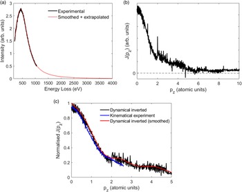
where “T” is the matrix transpose. It should be noted that  ${\bf J}$ here is an “isotropic” projected momentum density of states, since any anisotropy in J(pz) is not reproduced. The procedure for inverting the data is as follows. First a large enough range for pz is chosen, such that J(pz) decays to zero within the range. The Compton profile may have to be extrapolated to higher energy losses to accommodate the larger pz range. In our case, the maximum value of pz was set to 10 atomic units, and the Compton profile extrapolated to 4 keV, where the intensity was negligible (see Fig. 5a). A power law fit was used for the extrapolation. The extrapolated section of the Compton profile is smooth, while the measured part has some level of experimental noise. To avoid any artifacts this may cause the measured Compton profile was smoothed using a Savitzky–Golay filter (Savitzky & Golay, Reference Savitzky and Golay1964) and binned to increase the pixel size from 0.5 to 2.0 eV. Next the sampling of pz must be chosen; this determines the simulated energy resolution through equation (1c). The best results (i.e., minimal noise in ${\bf J}$) were obtained when the pz energy resolution matched the pixel size of the Compton profile (2.0 eV). This is likely related to the Moiré effects discussed earlier (see Section “Simulation Method”). The pz energy resolution depends on the Compton peak energy ΔE p, which is a variable, but here the ΔE p value for the unscattered beam was chosen as a guide, since for our case the unscattered beam has the highest intensity contribution (Fig. 4c).

Fig. 5. (a) The experimental dynamical Compton profile and its smoothing using the Savitzky–Golay method. The smoothed profile is extrapolated to 4 keV using a power law model. (b) The isotropic J(pz) obtained by inverting the dynamical Compton profile. (c) Superposition of the dynamical inverted and experimentally measured kinematical J(pz) profiles. Some of the extreme outliers in the former have been manually removed and the maximum value of J(pz) normalized for ease of visualization. Also shown is the Savitzky–Golay smoothed trace of the inverted J(pz) profile.
The inverted isotropic J(pz) for the dynamical Compton measurement (Fig. 4b) is shown in Figure 5b. There is noise introduced by the inversion algorithm, although the gross shape of J(pz) is as expected. In Figure 5c the inverted J(pz) is compared with the kinematical J(pz) from Figure 3d; some of the extreme outliers in the former profile have been manually removed for ease of visualization. The main J(pz) peak is similar for the two profiles, which suggests the inversion algorithm has removed much of the dynamical diffraction artifacts. The Savitzky–Golay smoothed, inverted J(pz) also shows smaller subsidiary maxima at pz values larger than 2 atomic units. Both the kinematical J(pz) profile, and the γ-ray results of Reed & Eisenberger (Reference Reed and Eisenberger1972), do not have sufficient sampling in this high momentum region to establish if these weaker maxima are a genuine feature of the sample, or alternatively, an artifact of the inversion routine.
Summary and Conclusion
Overcoming diffraction artifacts is crucial if electron Compton scattering is to be a robust tool for electronic structure analysis of crystalline materials. Several important breakthroughs were presented: first, a multislice algorithm was proposed for simulating the Compton profile measured under strong diffraction conditions. Dynamical scattering of the incident electron beam is modeled before and after the Compton energy loss event, an improvement over the simulations of Williams et al. (Reference Williams, Uppal and Brydson1987), which only considered the former. Simulated results agree well with experiment, although there is scope to improve the accuracy still further if interference effects can be included (Exner & Schattschneider, Reference Exner and Schattschneider1996). The simulations highlight the importance of both the incident electron beam and EELS detection geometries on the measured Compton profile. The former is restricted by the specimen diffraction conditions, but the latter can be optimized to suppress diffraction of the outgoing electron beam. Simulations are an important tool for assessing the role of dynamical scattering on Compton profiles, as well as selecting the optimum conditions for measurement. Furthermore, an inversion algorithm is developed for extracting the isotropic J(pz) from an experimental Compton profile distorted by dynamical diffraction. The isotropic J(pz) profile is prone to some noise from the inversion routine, although the gross features are reproduced. There is scope for more advanced inversion routines, possibly based on iterative methods, where the kinematically measured J(pz) profile is used as an initial solution that is iteratively refined to better fit the experimental data. A robust inversion algorithm could potentially be used to remove any diffraction artifacts still remaining after optimization of the experimental conditions, thereby enabling Compton data from crystalline materials that are largely error-free.
Acknowledgments
We are grateful to the UK Engineering and Physical Sciences Research Council (EPSRC) for supporting AT through the institutional doctoral training grant. Raw data and computer codes in this work can be accessed upon reasonable request by contacting the corresponding author.


 Open access