


Impact Statement
Global climate models can now be used to produce realistic simulations of climate. However, large uncertainties remain: for example, the estimated change in globally-averaged surface-temperature to a doubling of atmospheric CO2 varies between 2° and 6°C across leading models. Uncertainty in representing cumulus convection (think thunderstorm) is a major contributor to this spread: Scales at which they occur, 100 m–10 km, are too small to be resolved in global climate models, requiring their effects on larger scales to be approximated with simple models. Improving such approximations using new probabilistic machine-learning techniques, initial steps toward which are successfully demonstrated in this work will likely lead to improvements in the modeling of climate through improvements in the representation of cumulus convection.
1. Introduction and Problem Formulation
Over the past 70 years, there has been a concerted effort to develop first principles-based models of Earth’s climate. In this ongoing effort, current (state-of-the-art, SOTA) comprehensive climate models and Earth System Models (ESMs) have achieved a level of sophistication and realism that they are proving invaluable in improving our understanding of various processes underlying the climate system and its variability (Chen et al., Reference Chen, Rojas, Samset, Cobb, Niang, Edwards, Emori, Faria, Hawkins and Hope2021, p. 82). Limited by computational resources, however, most comprehensive climate simulations are currently conducted with horizontal grid spacings of between 50 and 100 km in the atmosphere. However, many atmospheric processes occur at much smaller scales. These include cumulus convection, boundary layer turbulence, cloud microphysics, and others. Even as resolutions continue to slowly increase, a number of these small-scale processes are not expected to be explicitly resolved in long-term simulations of climate for a long time. As such, the effects of such unresolved subgrid processes on the resolved scales have to be represented using parameterizations.
To wit, the evolution of temperature  $ T $ and moisture (represented by specific humidity) $ q $ may be written as (e.g., see Yanai et al., Reference Yanai, Esbensen and Chu1973; Nitta, Reference Nitta1977):
 $$ \frac{\partial T}{\partial t}+u\frac{\partial T}{\partial x}+v\frac{\partial T}{\partial y}-\omega {S}_p={q}_1, $$
 $$ \frac{\partial q}{\partial t}+u\frac{\partial q}{\partial x}+v\frac{\partial q}{\partial y}-\omega \frac{\partial q}{\partial p}=-{q}_2. $$
Here, ( $ u,v $) is the horizontal velocity field, $ \omega $ is the vertical velocity in pressure coordinates, $ {S}_p $ is static stability given by $ {S}_p=-\frac{T}{\theta}\frac{\partial \theta }{\partial p} $, where $ \theta $ is potential temperature and other notation is standard. To simplify notation, in the above equations all variables on the left-hand side (LHS) are understood to be variables at the resolved scale. With that convention, $ {q}_1 $ and $ {q}_2 $ are parameterizations that represent the effect of unresolved subgrid processes on the evolution of resolved scale temperature and moisture. (Additional mass and momentum conservation equations complete the system, e.g., by providing the evolution of ( $ u,v,\omega $).) For convenience, following Yanai et al. (Reference Yanai, Esbensen and Chu1973), we refer to $ {q}_1 $ as apparent heating and $ {q}_2 $ as apparent moisture sink.
In the above equations, terms on the LHS represent slow, large-scale dynamical evolution. Phenomenologically, when the large-scale dynamical evolution or forcing serves to set up conditions that are convectively unstable, the system responds by locally and intermittently forming cumulus convective updrafts that serve to locally resolve or eliminate the instability. Indeed, the interaction between the large-scale dynamics and small-scale intermittent moist nonhydrostatic cumulus response continues over a range of subgrid scales, from minutes and hundreds of meters to hours and up to 10 km. Thus, from the point of view of the equations above,  $ {q}_1 $ and $ {q}_2 $ represent the effect of unresolved cumulus and other subgrid processes on the evolution of the vertical profiles of environmental averages of the thermodynamic variables $ T $ and $ q $; $ {q}_1 $ is an apparent heating source and $ {q}_2 $ is an apparent moisture sink. In particular, $ {q}_1 $ comprises effects of radiative and latent heating and vertical turbulent heat flux, and $ {q}_2 $ effects of latent heating. The effects of horizontal turbulent transport are smaller in comparison and are therefore commonly neglected, as we do here.
In SOTA climate models, forward evolution of the atmospheric state over each timestep consists of a “dynamics” update (solving the mass and momentum equations and computing terms on the LHS of equations (1) and (2)) followed by a “physics” update. It is the “physics” update—effectively computing  $ {q}_1 $ and $ {q}_2 $—that implements the various schemes that capture the effect of unresolved dynamical and thermodynamic processes (e.g., turbulence transport including that of convective updrafts, various boundary layer processes, cloud microphysics, and radiation) on the resolved scales. Physics parameterizations in SOTA climate models tends to be one of the most computationally intensive parts (e.g., see Bosler et al., Reference Bosler, Bradley and Taylor2019; Bradley et al., Reference Bradley, Bosler, Guba, Taylor and Barnett2019). Furthermore, since traditional parameterizations are based on our limited understanding of the complex subgrid-scale processes, significant inaccuracies persist in the representation of microphysics, cumulus, boundary layer, and other processes (e.g., Sun and Barros, Reference Sun and Barros2014). Indeed, as pointed out by Sherwood et al. (Reference Sherwood, Bony and Dufresne2014), uncertainty in cumulus parameterization is a major source of spread in climate sensitivity of ESMs that are used for climate projections for the 21st century.
The recent explosion of research in machine learning (ML) has naturally led to the examination of the use of ML in alleviating both, shortcomings of human-designed physics parameterizations, and the computational demand of the “physics” step in climate models. In this context, recent research has focused on using short high-resolution simulations of climate that resolve convective updrafts, commonly called cloud-resolving models (CRMs) as ground truth for developing a computational-cheaper, unified machine-learned parameterization that replaces the traditional “physics” step. For example, using this approach, Brenowitz and Bretherton (Reference Brenowitz and Bretherton2018) were able to improve the representation of temperature and humidity fields when compared with traditional physics parameterizations.
In this study, instead of using output from high-resolution CRMs, since CRMs can themselves deviate from reality in many aspects (e.g., Lean et al., Reference Lean, Clark, Dixon, Roberts, Fitch, Forbes and Halliwell2008; Weisman et al., Reference Weisman, Davis, Wang, Manning and Klemp2008; Herman and Schumacher, Reference Herman and Schumacher2016; Zhang et al., Reference Zhang, Cook and Vizy2016), we train a ML model using reanalysis fields from the Modern-Era Retrospective Analysis for Research and Applications version 2 (MERRA-2, Rienecker et al., Reference Rienecker, Suarez, Gelaro, Todling, Bacmeister, Liu, Bosilovich, Schubert, Takacs, Kim, Bloom, Chen, Collins, Conaty, da Silva, Gu, Joiner, Koster, Lucchesi, Molod, Owens, Pawson, Pegion, Redder, Reichle, Robertson, Ruddick, Sienkiewicz and Woollen2011). Further, two similar input profiles (of temperature and humidity) can evolve differently due to chaotic subgrid cumulus dynamics and result in different output profiles (of apparent heating and apparent moisture sink). As such, we estimate  $ {q}_1 $ and $ {q}_2 $ using a probabilistic ML model. This choice is also consistent with the suggestion that a stochastic approach is likely more appropriate for parameterizations in terms of reducing the uncertainties stemming from the lack of scale separation between resolved and unresolved processes (e.g., see Duan and Nadiga, Reference Duan and Nadiga2007; Nadiga and Livescu, Reference Nadiga and Livescu2007; Nadiga, Reference Nadiga2008; Palmer, Reference Palmer2019).
2. The Tropical Eastern Pacific, Data and Preprocessing
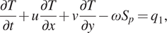
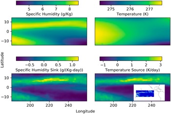
The inter-tropical convergence zone (ITCZ) is one of the easily recognized large-scale features of earth’s atmospheric circulation. It appears as a zonally elongated band of clouds that at times even encircles the globe. It comprises of thunderstorm systems with low-level convergence, and intense convection and precipitation, The domain we choose—the region of Eastern Pacific, 15S–15N and 180–100.25 W—includes both a segment of the more coherent northern branch of the ITCZ as a band across the northern part of the domain, and a segment of the more seasonal southern branch in the southwestern part of the domain. In the top-left panel of Figure 1, which shows the 2003 annual mean of column-averaged specific humidity, the ITCZ is contained in the broad and diffuse bands of high moisture seen in yellow. While not evident in the equivalently averaged temperature field (top-right), it is better identified in the  $ {q}_1 $ and $ {q}_2 $ fields (bottom row; see later). To aid in geo-locating the domain considered and the ITCZ, the inset in the bottom-right panel shows the $ {q}_1 $ field for January 1, 2003 on a map with the coastlines of the Americas.
Figure 1. Preprocessing of MERRA2 data in the tropical Eastern Pacific. Top: Annual mean of column-averaged specific humidity (left) and temperature (right) in the Eastern Pacific. Bottom: Annual mean of apparent moisture sink (left) and apparent heating (right). To aid in geo-locating the domain considered and the ITCZ, the inset in the bottom-right panel shows the  $ {q}_1 $ field for January 1, 2003 on a map.
Whereas the timescales of convective updrafts range from minutes to hours, the reanalyzed fields under NASA’s Modern-Era Retrospective analysis for Research and Applications, version 2 (MERRA2) project are made available at a sampling interval of 3 hr. Nevertheless, the reanalyzed fields contain the averaged effects of convective updrafts and other subgrid processes. First, we use the  $ T $, $ q $, and ( $ u,v,\omega $) fields to estimate $ {q}_1 $ and $ {q}_2 $ using equations (1) and (2). On so doing, we find that there are numerous instances wherein the diagnosed $ {q}_1 $ and $ {q}_2 $ fields are dominated by the vertical advection of temperature and specific humidity, respectively, and which are themselves much larger than the horizontal advection terms and the temporal tendency terms. Furthermore, in such cases, the vertical distributions of $ {q}_1 $ and $ {q}_2 $ were found to be highly correlated to the vertical distributions of vertical advection of temperature and specific humidity respectively. We proceed to further investigate this aspect of the diagnosed diabatic sources in order to establish that they are not mere artifacts before proceeding with modeling them.
MERRA2 is a reanalysis product in the sense that it uses an atmospheric general circulation model (AGCM), the Goddard Earth Observing System version 5 (GEOS-5), and assimilates observations to produce interpolated and regularly gridded data (Rienecker et al., Reference Rienecker, Suarez, Gelaro, Todling, Bacmeister, Liu, Bosilovich, Schubert, Takacs, Kim, Bloom, Chen, Collins, Conaty, da Silva, Gu, Joiner, Koster, Lucchesi, Molod, Owens, Pawson, Pegion, Redder, Reichle, Robertson, Ruddick, Sienkiewicz and Woollen2011). While vertical motion is intimately linked to the stability of the atmosphere given stratification in the vertical, and is key to the formation of cumulus, vertical velocity is usually not directly measured. It is indeed the case that direct observations of vertical motion are not part of the data that are assimilated by the GOES-5 AGCM to produce MERRA2. As such, to examine whether the high-frequency (temporal), high-wavenumber (spatial) component of the inferred vertical (pressure) velocity of MERRA2 (components in which the confidence tends to be lower than in the slower, larger-scale components) leads to the correlation mentioned above, we consider further spatiotemporal averaging of the MERRA2 fields from a native resolution of 0.5°  $ \times $ 0.625° at 3 hr to a daily average at a coarsened resolution of 1° $ \times $ 1° (e.g., Sun and Barros, Reference Sun and Barros2015). The persistence of the correlations, however, suggests that the correlations are likely real.
All fields are considered on MERRA2’s native vertical grid (pressure levels) and we confine attention to the troposphere, defined here for convenience as pressure levels deeper than 190 mbar (hPa); there are 31 such levels. Figure 1 shows the annual and vertical average of specific humidity (top-left), temperature (top-right), diagnosed specific humidity sink (bottom-left), and temperature source (bottom-right). The ITCZ is seen to be better defined in the diagnosed (bottom) fields and its structure in  $ {q}_1 $ and $ {q}_2 $ is also seen to be highly correlated.
3. Generative Adversarial Networks
The governing equations would be closed if we are able to express the three-dimensional fields  $ {q}_1 $ and $ {q}_2 $ in terms of the resolved (3D) variables; given that they are not closed, we proceed to find such closures using machine-learning. However, given the physics of the problem described previously, the dominant variation of such relationships is captured by the column-wise variation of $ {q}_1 $ and $ {q}_2 $ in terms of the column-wise variation of $ T $ and $ q $. Furthermore, as alluded to earlier, we should not expect unique functional relationships between the predictands and predictors. As such a probabilistic ML framework is called for. That is, instead of learning maps,
 $$ \left[T(p),q(p)\right]\mapsto \left[{q}_1(p),{q}_2(p)\right], $$
we are led to want to learn the conditional probability,
 $$ P\left(\Big[{q}_1(p),{q}_2(p)\Big]|\Big[T(p),q(p)\Big]\right), $$
the probability of  $ \left[{q}_1(p),{q}_2(p)\right] $ occurring given the occurrence of conditions $ \left[T(p),q(p)\right] $.
In this setting, a conditional generative model is required, since in essence, a generative model learns a representation of the unknown probability distribution of the data. Different classes of generative models have been developed and they can range from generative adversarial networks (GANs) (Goodfellow et al., Reference Goodfellow, Pouget-Abadie, Mirza, Xu, Warde-Farley, Ozair, Courville and Bengio2014) to variational autoencoders (Kingma and Welling, Reference Kingma and Welling2013) to continuous normalizing flows (Rezende and Mohamed, Reference Rezende and Mohamed2015) to diffusion maps (Coifman and Lafon, Reference Coifman and Lafon2006) and others. However, we choose GANs since they have been investigated more extensively than the others. As a class of generative models, GANs are trained using an adversarial technique: while a discriminator continually learns to discriminate between the generator’s synthetic output and true data, given a noise source, the generator progressively seeks to fool the discriminator by synthesizing yet more realistic samples. The (dual) learning progresses until quasi-equilibrium is reached (see Figure 2a for an example of this in the current setup), wherein the discriminator’s feedback to the generator does not permit further large improvements of the generator, but rather leads to stochastic variations that explore the local basin of attraction. In this state, the training of the generator may be considered as successful to the extent that the discriminator has a hard time, both, discriminating between true samples and fake samples created by the trained generator, and learning further to discriminate them.
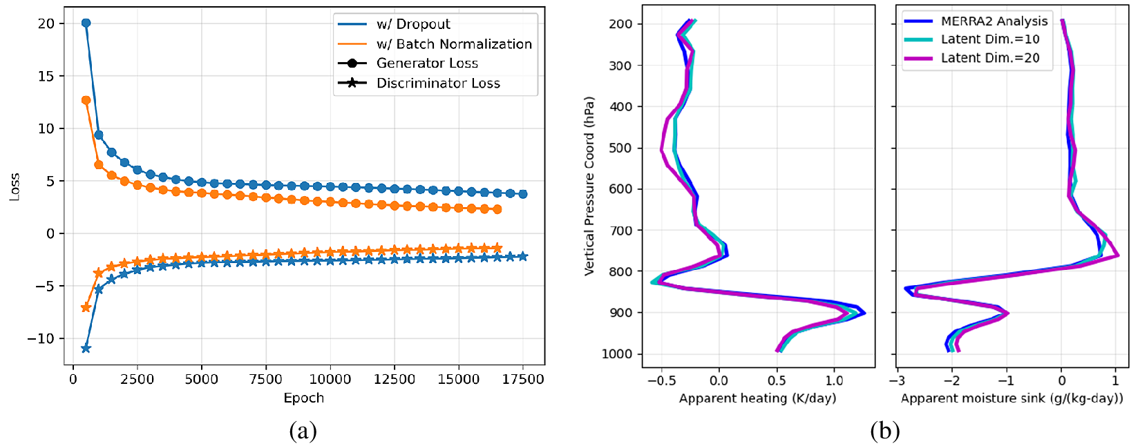
Figure 2. (a) Training loss with dropout (blue) and with batch normalization as a function of training epoch. Both generator and discriminator losses are shown and the training is seen to continue stably over large numbers of epochs. (b) Comparison of vertical distribution of cGAN predictions against reference MERRA2 analysis. Averages over test set of apparent heating (left) and apparent moisture sink (right) are compared. Teal (Magenta) values are for the case when the dimension of the noise vector is 10 (20).
Initially, the training of GANs was problematic in that they commonly suffered from instability and various modes of failure. One of the approaches developed in response to the problem of instability in the training of GANs was the Wasserstein GAN (WGAN) (Arjovsky and Bottou, Reference Arjovsky and Bottou2017) The WGAN approach leverages the Wasserstein distance (Kantorovitch, Reference Kantorovitch1958) on the space of probability distributions to produce a value function that has better theoretical properties, and requires the discriminator (called the critic in the WGAN setting) to lie in the space of 1-Lipschitz functions. While the WGAN approach made significant progress toward stable training of GANs and gained popularity, subsequent accumulating evidence revealed that the WGAN approach could sometimes generate only poor samples or, worse, even fail to converge. In further response to this aspect of WGANs, a variation of the WGAN was proposed by Gulrajani et al. (Reference Gulrajani, Ahmed, Arjovsky, Dumoulin and Courville2017): while in the original WGAN, a weight-clipping approach was used to ensure that the critic lay in the space of 1-Lipschitz functions, the new approach used a gradient penalty term in the critic’s loss function to satisfy the 1-Lipschitz requirement. As such this approach was called the Wasserstein GAN with gradient penalty (WGAN-GP).
3.1. Architecture and loss functions
In the conditional version of the WGAN-GP we use, besides the input and output layers, the generator and critic networks each consist of three fully connected feed-forward hidden layers (multilayer perceptron architecture). The hidden layers have 512 neurons each with 10% dropout, and use rectified linear unit (ReLU) activation functions while the input and output layers are linear. The noise sample was concatenated to the condition vector for input to the generator. And, the condition vector was concatenated to the real or generated sample to form the input to the critic network.
The dataset consisted of 864,000 datapoints (30 latitude bins, 80 longitude bins, and 360 daily averages [1/4–12/29]) with 62 conditions representing temperature and humidity at 31 vertical pressure levels. The target variables were  $ {q}_1 $ and $ {q}_2 $ at the same 31 vertical levels. To account for the typical dominant nature of the seasonal component of climate variability, the dataset was split into quarters, the first 70 days of each quarter were used for training and the subsequent 20 days of each quarter constituted the test set. Training data was scaled to a mean of zero and unit standard deviation (standardized), and the same, learned, transformation was applied to the test data. Data was inverse transformed prior to plotting and metric calculations. Training data was split into 100 mini-batches per epoch.
The generator and critic loss functions were as proposed in Gulrajani et al. (Reference Gulrajani, Ahmed, Arjovsky, Dumoulin and Courville2017) with gradient penalty added to the critic loss. Training was performed with an Adam optimizer with momentum parameters ( $ \beta $s) set to 0.5 and 0.9. The coefficient of gradient penalty was set at 0.1. We note that when using the same generator and critic architectures, but with other data (Hossain et al., Reference Hossain, Nadiga, Korobkin, Klasky, Schei, Burby, McCann, Wilcox, De and Bouman2021), we have found robust behavior of the predictions over a wide range of values for the coefficient of gradient penalty (0.01–10). A learning rate of 1e-3 was used. The generator was only updated every fifth step in order to allow the critic to learn the Wasserstein distance function better before updating the generator. Once training was complete, the test conditions along with noise samples were fed to the generator to produce results that we discuss in the next section.
Variations of hyperparameter considered consisted of number of neurons in each layer, number of layers, activation function, coefficient of gradient penalty in discriminator loss, dropout and batch normalization layers in generator, and the dimension of the noise vector input to the generator. No sensitive dependencies were found. Furthermore, a validation set was not used for the reason that the training of the cGAN was stable and no special stopping criterion was used. For example, the averaged generator and discriminator loss functions were monotonic and could be continued for tens of thousands of epochs (see Figure 2a for an example).
4. Results
Given the physics of the problem, and as described earlier, we focus on the vertical distributions of apparent heating and moisture sink, conditioned on the vertical distributions of temperature and specific humidity. Figure 2b shows comparisons of the vertical distribution of cGAN predictions against reference MERRA2 analysis. Here, averages over the test set are compared, with apparent heating shown in the left panel and the apparent moisture sink shown in the right panel. Two sets of cGAN predictions are shown with the only change being the dimension of the noise vector (cyan: 10, magenta: 20). The overall structure of the vertical distribution of both heating and moisture sink are reasonably well captured by the cGAN predictions with no indication of bias.
In more detail, in Figure 3a, we consider the probability distributions over the test set at each pressure level with red indicating high probability and blue indicating low probability. Apparent heating is shown in the left column and apparent moisture sink is in the right column. Reference MERRA2 analysis is shown in the top row and cGAN predictions (noise vector dimension 10) are in the bottom row. The pdfs of the cGAN predictions are seen to compare well with the reference MERRA2 analysis. In particular, the predictions capture the skewed nature of the distributions well. However, the regions of high probability (width of red regions) in the pdfs of the cGAN predictions of heating, are seen to be slightly sharper than in MERRA2 analysis. (With batch normalization, while the width of the mode region is as in MERRA2, a different minor discrepancy is seen: there are sharper jumps in the vertical.) For reference, at a yet more detailed level, we show stochastic ensembles of predictions at four randomly chosen test conditions in Figure 3b. The reference MERRA2 profiles are shown in blue and the predictions are in orange. Note that while the cGAN predictions sometimes appear as a thick orange line, they are actually an ensemble of thin lines. The stochastic ensemble was obtained by holding the test condition fixed while repeatedly sampling the noise vector. More often, the cGAN predictions are seen to better capture the slower variations.
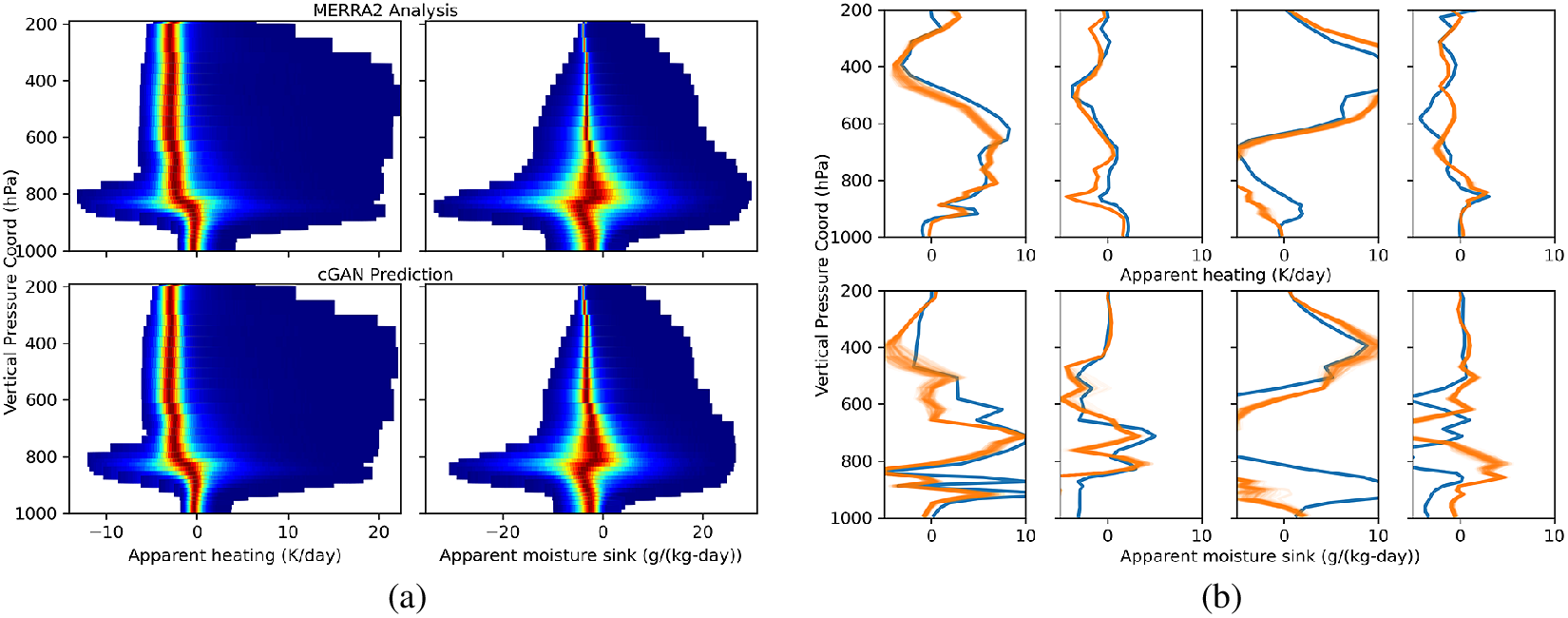
Figure 3. (a) The probability distribution functions (pdf; red: high probability; blue: low probability) over the test set are computed at each pressure level and compared against the MERRA2 pdfs. The variable depth of the MERRA2 vertical layers is apparent in these figures. Apparent heating is shown in the left column and apparent moisture sink is shown in the right column. Reference MERRA2 analysis is shown in the top row and cGAN predictions (noise vector dimension of 10) are shown in the bottom row. (b) A stochastic ensemble of cGAN predictions is shown for four random instances in the test set. The top row is for heating whereas the bottom row is for moisture sink. The reference MERRA2 profiles are shown in blue and the predictions are in orange.
5. Conclusion
The tropical Eastern Pacific is an important region for global climate and contains regions of intense tropical convection—segments of the ITCZ. Adopting a framework of apparent heating and apparent moisture sink to approximately separate the effects of dynamics and column physics, we diagnosed the “physics” sources using the MERRA2 reanalysis product in a preprocessing step. We performed the analysis at MERRA2’s native spatiotemporal resolution, and then at a significantly coarser resolution. In both cases, we found that the heating and moisture sink were highly correlated with vertical advection of temperature and humidity (~0.9, and  $ -0.7 $), respectively.
Thereafter, we designed a probabilistic ML technique to learn the distribution of the heating and moisture sink profiles conditioned on vertical profiles of temperature and specific humidity. This was based on a Wasserstein Generative Adversarial Network with gradient penalty (WGAN-GP). After successfully training the cGAN, we were able to demonstrate the viability of the methodology to learn unified stochastic parameterizations of column physics by comparing predictions using test conditions against reference MERRA2 analysis profiles. We expect this work to add to the growing body of literature (e.g., Krasnopolsky et al., Reference Krasnopolsky, Fox-Rabinovitz, Hou, Lord and Belochitski2010, Reference Krasnopolsky, Fox-Rabinovitz and Belochitski2013; Brenowitz and Bretherton, Reference Brenowitz and Bretherton2018; O’Gorman and Dwyer, Reference O’Gorman and Dwyer2018; Rasp et al., Reference Rasp, Pritchard and Gentine2018, and others) that seeks to develop machine-learned column-physics parameterizations toward alleviating both, shortcomings of human-designed physics parameterizations, and the computational demand of the “physics” step in climate models.
We conclude by mentioning a few issues that need further investigation. Given the diversity of behavior (e.g., ITCZ vs. non-ITCZ regions), it remains to be seen if adding velocity fields as predictors will improve performance. Training over ITCZ regions and testing elsewhere and other such combinations are likely to render further insight into the parameterizations. The stochastic ensemble our method produces, for example, like in Figure 3b, can be readily subject to reliability and other analyses using tools developed in the context of probabilistic weather forecasts (e.g., see Nadiga et al., Reference Nadiga, Casper and Jones2013; Luo et al., Reference Luo, Nadiga, Ren, Park, Xu and Yoo2022, and references therein). We anticipate that such analyses will help us better understand the role played by the dimension of the latent space used in generative modeling. Finally, the stability of the machine-learned parameterization in a GCM setting is an important issue. For example, Brenowitz and Bretherton (Reference Brenowitz and Bretherton2018) find this to be a problem when they learn deterministic parameterizations from CRM-based data. They circumvent the problem by changing the problem formulation to include time integration of the temperature (in their case static stability) and moisture equations and changing the loss function to penalize deviations of the predictions of  $ T $ and $ q $ at multiple times in a cumulative sense. It remains to be seen if the stochastic parameterizations learned using a probabilistic ML methodology, as we do presently, can provide an alternative way of addressing the stability issue.
Author Contributions
Conceptualization: B.T.N.; Data curation: B.T.N., X.S.; Data visualization: B.T.N.; Methodology: B.T.N., C.N.; Writing—original draft: B.T.N. All authors approved the final submitted draft.
Competing Interests
The authors declare no competing interests exist.
Data Availability Statement
MERRA2 data used in this work is available and can be downloaded at https://disc.gsfc.nasa.gov/datasets?project=MERRA-2.
Funding Statement
This research was supported under the U.S. Department of Energy (DOE), Office of Science’s Scientific Discovery through Advanced Computation (SciDAC4) program under project “Non-Hydrostatic Dynamics with Multi-Moment Characteristic Discontinuous Galerkin Methods (NH-MMCDG).”
Provenance
This article is part of the Climate Informatics 2022 proceedings and was accepted in Environmental Data Science on the basis of the Climate Informatics peer review process.


 Open access