


Introduction
The substantial advances of microscopy techniques and aberration-corrected electron optics since the second half of the last century have made it possible to probe materials at atomic resolution (Hansma et al., Reference Hansma, Elings, Marti and Bracker1988; Haider et al., Reference Haider, Uhlemann, Schwan, Rose, Kabius and Urban1998; Batson et al., Reference Batson, Dellby and Krivanek2002), which opened up an era where materials can be studied down to the level of single atoms (Krivanek et al., Reference Krivanek, Chisholm, Nicolosi, Pennycook, Corbin, Dellby, Murfitt, Own, Szilagyi, Oxley, Pantelides and Pennycook2010). Aberration-corrected scanning transmission electron microscopes (STEMs) have made it routine to acquire atomic-resolution images, image series, and spectroscopic data of crystalline materials. This information provides deep insights into the atomic structure of lattice defects, local atomic ordering, or complex interface structures, such as grain-boundary phase transitions (Reference Meiners, Frolov, Rudd, Dehm and LiebscherMeiners et al., Reference Meiners, Duarte, Richter, Dehm and Liebscher2020a, Reference Meiners, Frolov, Rudd, Dehm and Liebscher2020b) and three-dimensional atomic arrangements of nanoparticles (Van Aert et al., Reference Van Aert, Batenburg, Rossell, Erni and Van Tendeloo2011).
As more and more atomic scale data becomes available, we are facing the challenge of efficiently analyzing these large data sets generated even in a single experiment (Belianinov et al., Reference Belianinov, Vasudevan, Strelcov, Steed, Yang, Tselev, Jesse, Biegalski, Shipman, Symons, Borisevich, Archibald and Kalinin2015; Spurgeon et al., Reference Spurgeon, Ophus, Jones, Petford-Long, Kalinin, Olszta, Dunin-Borkowski, Salmon, Hattar, Yang, Sharma, Du, Chiaramonti, Zheng, Buck, Kovarik, Penn, Li, Zhang, Murayama and Taheri2020). Typical tasks are to discover and label recurrent patterns, to identify features of possible interest, to classify and quantify such features for large data sets, and to collect the corresponding statistics. Machine-learning methods have been shown to be effective in speeding up and automatizing the data processing in various microscopy-related problems (Madsen et al., Reference Madsen, Liu, Kling, Wagner, Hansen, Winther and Schiøtz2018; Kalinin et al., Reference Kalinin, Lupini, Dyck, Jesse, Ziatdinov and Vasudevan2019; Roberts et al., Reference Roberts, Haile, Sainju, Edwards, Hutchinson and Zhu2019; Kaufmann et al., Reference Kaufmann, Zhu, Rosengarten, Maryanovsky, Harrington, Marin and Vecchio2020; Spurgeon et al., Reference Spurgeon, Ophus, Jones, Petford-Long, Kalinin, Olszta, Dunin-Borkowski, Salmon, Hattar, Yang, Sharma, Du, Chiaramonti, Zheng, Buck, Kovarik, Penn, Li, Zhang, Murayama and Taheri2020; Ziatdinov et al., Reference Ziatdinov, Fuchs, Owen, Randall and Kalinin2020).
We will focus in the following on analyzing high-angle annular dark-field (HAADF) STEM images of complex crystalline materials at atomic resolution. The HAADF-STEM data set consists of the detector signal intensity as function of the scanning position of the focused electron beam. Such data is typically displayed as a gray-scale image, which allows us to exploit the techniques and terminology used for digital image processing in general. Conversely, the algorithms described in the following are well suited to comparable data sets from other atomic-scale imaging techniques, for example, atomic force microscopy (AFM), high-resolution transmission electron microscopy (HRTEM), and scanning tunneling microscopy (STM). Within the scope of the present work, however, we have not tested the methods on data sets other than those coming from HAADF-STEM. We are also interested in image series taken for the same area repeatedly—equivalent to a (short) video, where the single image is usually called a frame.
Despite all analogy to images in general, the experimental signal typically comes with much higher levels of noise compared with photographic images. Tolerance to the experimentally characteristic noise is, therefore, desirable. The noise level can be influenced by the experimental conditions. For instance, short exposure times imply higher noise levels due to the stochastic nature of electron scattering. On the other hand, reduced exposure times improve the time resolution of image series and limit beam damage (Egerton et al., Reference Egerton, Li and Malac2004). At present, experimental conditions are chosen prior to data analysis. In perspective, however, on-the-fly analysis (and hence fast processing) will open new opportunities to optimize the trade-off by adapting the experimental conditions directly to the needs of the on-going analysis.
For polycrystalline samples, a crucial subtask is to identify and mark all regions that share a common characteristic, which is called image segmentation. A successful segmentation may then serve multiple purposes. First, it can help to visualize larger structures inherent to the data, but not always visible to the human eye from a gray-scale image alone. Second, segmentation information can be used to improve the signal-to-noise ratio in other data channels in STEM (which share the  $x,\; y$ beam position), by selectively accumulating weak signals from within each segment. Third, if the segments map well onto the underlying crystallography, measuring the segmented areas and boundaries yields direct quantification of microstructural properties. Last, the certainty of the classifier underlying the segmentation can be used to detect “unusual” spots within a region, and hence help to find a relevant isolated outlier, that is, a defect.
Segmentation is also an important principle of human visual perception, as it helps us see “at a glance” different hierarchical structures, both in daily life and in scientific analysis. Not surprisingly, it is one of the most researched topics of machine learning on images. Supervised algorithms are trained to recognize and label the regions from a pre-defined set of possible patterns (Arganda-Carreras et al., Reference Arganda-Carreras, Kaynig, Rueden, Eliceiri, Schindelin, Cardona and Sebastian Seung2017; Vu et al., Reference Vu, Graham, Kurc, To, Shaban, Qaiser, Koohbanani, Khurram, Kalpathy-Cramer, Zhao, Gupta, Kwak, Rajpoot, Saltz and Farahani2019). Unsupervised algorithms aim at distinguishing features from the data at hand (Nock & Nielsen, Reference Nock and Nielsen2004; Mancas et al., Reference Mancas, Gosselin and Macq2005; Sadowski et al., Reference Sadowski, Broadbridge and Daponte2006; Navlakha et al., Reference Navlakha, Ahammad and Myers2013; Borodinov et al., Reference Borodinov, Tsai, Korolkov, Balke, Kalinin and Ovchinnikova2020).
Since the difference between crystal patterns in atomic-resolution images is dominated by the local arrangement of atomic columns, conventional segmentation methods such as thresholding (Mancas et al., Reference Mancas, Gosselin and Macq2005; Sadowski et al., Reference Sadowski, Broadbridge and Daponte2006) and region merging (Nock & Nielsen, Reference Nock and Nielsen2004; Navlakha et al., Reference Navlakha, Ahammad and Myers2013) are not straightforwardly applicable to go beyond the detection of single columns. An alternative is the use of suitable descriptors (Borodinov et al., Reference Borodinov, Tsai, Korolkov, Balke, Kalinin and Ovchinnikova2020). A typical descriptor-based unsupervised segmentation proceeds as follows. (1) The algorithm computes local features for small areas (patches) across the entire image. The feature values for each patch define a “point” in feature space. (2) This image representation is projected to a subspace of reduced dimensionality based on the variance of all available points. (3) Clustering analysis is used to further partition feature space. (4) The algorithm classifies the original patches by using a metric to identify the “nearest” cluster.
Supervised algorithms also use descriptor-based classifiers, but the classification nowadays employs nonlinear mappings (e.g., deep neural networks) trained on pre-labeled data. Such machine-learning methods (Arganda-Carreras et al., Reference Arganda-Carreras, Kaynig, Rueden, Eliceiri, Schindelin, Cardona and Sebastian Seung2017; Vu et al., Reference Vu, Graham, Kurc, To, Shaban, Qaiser, Koohbanani, Khurram, Kalpathy-Cramer, Zhao, Gupta, Kwak, Rajpoot, Saltz and Farahani2019) have been explored in the biological community to segment tissue images, which require a large amount of labeled data to train a classification model or a neural network, which are not yet available for atomic scale images of crystalline matter. While good progress has been demonstrated in the literature, the drawback of supervised models is that data labeling is time-consuming, and that the supervised models may interpret patterns absent from training data in unexpected ways.
In the context of imaging crystals, the desired segmentation must reflect the known hierarchical structure of solid matter, such as crystal lattices, lattice defects, crystal grains, microstructures, or texture. It should do so in a transparent manner, that is, the individual steps listed above should be accessible to the human scientist to ensure a correct interpretation, and reversely, guarantee that the segmentation proceeds in the intended way.
To summarize the requirements at this point, we aim at a segmentation algorithm that (1) detects crystallographic features of the imaged area without prior knowledge, (2) is robust against relatively high noise levels, (3) is computationally fast, and (4) is interpretable in each of its stages. With these criteria in mind, we developed an unsupervised segmentation algorithm based on local symmetry in atomic-resolution images, which is encoded in local descriptors. By design, the algorithm autonomously detects distinct features with characteristic local symmetry of crystalline material, but simultaneously provides a high degree of flexibility and controllable noise tolerance. This control is achieved by setting manually the hyperparameters of the algorithm as discussed in detail in the following, and summarized in Appendix A. In the future, some of these hyperparameters might be set automatically from the data set at hand. We furthermore propose an extension in order to efficiently segment large-scale image sequences containing similiar features that evolve over time, for example, in in situ STEM videos captured at atomic resolution. The main steps of our workflow include feature extraction via symmetry operations, dimension reduction of local descriptors, clustering analysis to partition feature space, stride and upsampling, and separability analysis. They are summarized in Figure 1 and detailed in the next section.
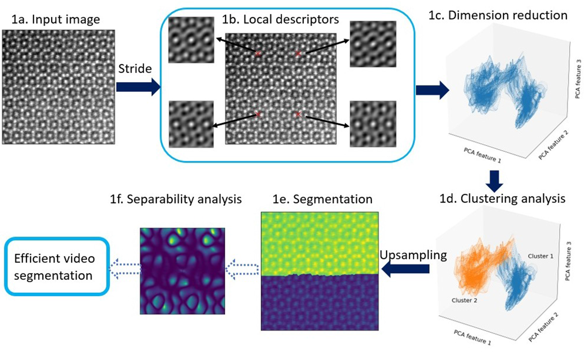
Fig. 1. Main steps in our image-segmentation workflow. An atomic-resolution HAADF-STEM image of an iron–niobium intermetallic compound with two phases ( $\mu$ phase and Laves phase) is used for demonstration. The hyperparameters in the workflow are described in Appendix A. (1a) Input image, for example, HAADF-STEM, AFM, or STM image. (1b) Extracting local descriptors via symmetry operations. Local descriptors for translational symmetries (cf. Section “Extracting features via translation operations”, Fig. 3) of four selected pixels are visualized here. (1c) Dimension reduction with principal component analysis (PCA). Here, three components are employed to obtain the scatter plot (cf. Section “Dimension reduction”). (1d) K-means clustering analysis to separate patterns in feature space. Two clusters are shown in this plot, while more clusters might be involved in other cases. (1e) Segmented image plotted as superposition of pattern labels and raw image intensities. (1f) Separability analysis: Here, we show a separability map for all possible translational operations. We may select symmetry operations with best separability to segment more images with similiar features. The application to an in situ high-resolution TEM video sequence is discussed in the result section and shown in the Supplementary material.
Methodology
Feature Extraction via Symmetry Operations
We aim at segmenting the microscopy images into multiple crystal patterns that are different in terms of symmetry, that is, locally self-similar under certain coordinate transformations (the symmetry operations). Four types of symmetry operations are involved in the two-dimensional (2D) crystal patterns: pure translations, rotations, reflections, and glide-reflections. The main idea of symmetry-based feature extraction is to take a finite set of candidate symmetry operations, apply them all to a small region (a “patch”) of the image and score the degree to which the symmetry applies. Denoting the 2D coordinate of the patch by  ${\bf r} = ( x,\; y)$, the associated coordinate transformations read as follows.
Translation by vector  ${\bf t}$:
 $${\bf r} \rightarrow {\bf r} + {\bf t}.$$
 Rotation by angle  $\alpha$ around center ${\bf c}$:
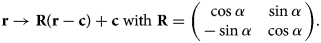 $${\bf r} \rightarrow {\bf R}( {\bf r} - {\bf c}) + {\bf c} \; \hbox{with}\; {\bf R} = \left(\matrix{ \cos \alpha & \sin \alpha\cr - \sin \alpha & \cos \alpha }\right).$$
 (Glide) reflection at an axis  ${\bf c} \cdot \left(\matrix{-\sin \beta \cr \cos \beta}\right) = D$, which forms angle $\beta$ to the $x$-axis and lies at oriented distance $D$ from the origin:
 $${\bf r} \rightarrow {\bf M}( {\bf r} - {\bf c}) + {\bf c} + {\bf t} = {\bf M} {\bf r} + {\bf t}',$$
where  ${\bf c}$ is any point on the axis, and ${\bf t}$ the glide along the axis, with
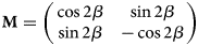 $${\bf M} = \left(\matrix{ \cos 2\beta & \sin 2\beta \cr \sin 2\beta & -\cos 2\beta }\right)$$
and
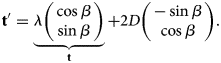 $${\bf t}' = \underbrace{\lambda \left(\matrix{ \cos \beta \cr \sin\beta }\right)}_{{\bf t}} + 2D \left(\matrix{ -\sin \beta\cr \cos \beta }\right).$$
 When the glide parameter  $\lambda$ is zero, this is a pure reflection.
As the parameters of these symmetry operations ( ${\bf t}$, ${\bf c}$, $\alpha$, $\beta$, $D$, and $\lambda$) may take various values, there are many possible symmetry operations. This yields a symmetry-score vector as a local descriptor for the chosen patch. In other words, the candidate symmetry operation together with the symmetry scoring makes a local-symmetry-feature extractor. We shift the extractor across the entire image in order to extract the local-symmetry information everywhere in the image. The schematic diagram for this calculation is shown in Figure 2.
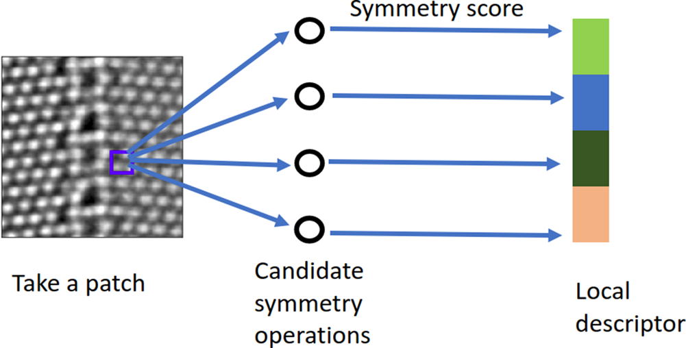
Fig. 2. A schematic diagram illustrating the symmetry-based local descriptors.
To quantify the degree to which a candidate symmetry operation,  $O$, matches the image locally, we compare how well a small patch of the image, $P_{x, y}$, centered at the pixel $( x,\; y)$, maps to the actual image at the transformed coordinates, $OP_{x, y}$. The similarity between the two patches is determined via Pearson's correlation coefficient. Pearson's correlation coefficient takes a value in the range from $-$1 to 1, where larger values mean stronger similarity. To compute it, we first evaluate the mean intensities
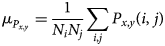 $$\mu_{P_{x, y}} = {1\over N_i N_j}\sum_{i, j}P_{x, y}( i,\; j) $$
and, analogously,  $\mu _{OP_{x, y}}$. $P_{x, y}( i,\; j)$ are the intensities at the position $( i,\; j)$ in their relative coordinates. The Pearson's correlation coefficient is then evaluated according to
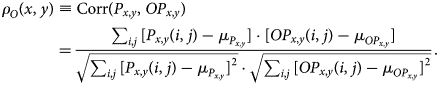 $$\rho_O( x,\; y) \equiv {\rm Corr}( P_{x, y},\; OP_{x, y} ) = {\sum_{i, j}[ P_{x, y}( i,\; j) -\mu_{P_{x, y}}] \cdot[ OP_{x, y}( i,\; j) -\mu_{OP_{x, y}}{}] \over \sqrt{\sum_{i, j}[ P_{x, y}( i,\; j) -\mu_{P_{x, y}}] ^{2}} \cdot \sqrt{\sum_{i, j}[ OP_{x, y}( i,\; j) -\mu_{OP_{x, y}}] ^{2}} }.$$
We emphasize that the relative coordinates are not necessarily Cartesian coordinates. We employ polar coordinates and circular-shape patches to handle rotation and reflection operations. The intensity at polar grids are obtained through cubic spline interpolation as implemented in scipy (Pedregosa et al., Reference Pedregosa, Varoquaux, Gramfort, Michel, Thirion, Grisel, Blondel, Prettenhofer, Weiss, Dubourg, Vanderplas, Passos, Cournapeau, Brucher, Perrot and Duchesnay2011).
In the remainder of this subsection, we employ the general procedure illustrated in Figure 2 to obtain two groups of local descriptors. The application to the translation operations provides us with local descriptors that have natural translational invariance within the same crystal pattern. In contrast, the local descriptors that are obtained by performing the rotation and reflection operations are not translationally invariant. In the latter case, we add a so-called max-pooling step to enforce the translational invariance, similar to the treatment adopted in convolutional neural networks (Boureau et al., Reference Boureau, Ponce and Lecun2010). In max-pooling, the maximum value of the symmetry score inside a “pooling window” becomes the new feature to characterize local symmetry. Max-pooling is usually employed to coarse-grain from single pixels to pooling window resolution. We generalize this to an arbitrary spatial grid independent of the pooling window size by employing a moving pooling window, always centered at the grid point, where the pooling windows of neighboring grid points may overlap.
Extracting Features via Translation Operations
Based on the general procedure illustrated in Figure 2, we calculate the translational-symmetry-based local descriptors at the pixel  $( x,\; y)$ as follows. We select a patch centered at $( x,\; y)$, $P_{x, y}( i,\; j)$, where $i$ and $j$ are the coordinates in the Cartesian coordinate system with the origin at $( x,\; y)$. The absolute value of $i$ (
$i$ ( $j$) is not larger than the half height (width) of the patch, $\vert i\vert \leq p_x$ and $\vert j\vert \leq p_y$. We denote the translation shift as $T_{m, n}$, which shifts the patch by $m$ pixels vertically and by $n$ pixels horizontally. The transformed patch by this operation is simply the patch located at $( x + m,\; y + n)$, namely, $T_{m, n}P_{x, y} = P_{x + m, y + n}$. Substituting this into equation (2), we obtain the symmetry score for the translation operation $T_{m, n}$,
 $$\rho_{T_{m, n}} ( x,\; y) = {\rm Corr}( P_{x, y},\; P_{x + m, y + n}) .$$
 In practice, we confine the translation shift in a region of shape  $( 2w_x + 1,\; 2w_y + 1)$, that is, $\vert m\vert \leq w_x$ and $\vert n\vert \leq w_y$, and select uniformly a fixed number $N$ of translation shifts in this region. The symmetry scores for the selected translation shifts form a feature vector of length $N$, which is the local descriptor characterizing the local translational symmetries.
In our package (Wang, Reference Wang2021a, Reference Wang2021b, Reference Wang2021c), we implement the translation-based local descriptors with two methods, the direct and the fast Fourier transform (FFT) based ones. In the direct method, we evaluate the symmetry score equation (3) for the selected translation shifts directly in the low-level C code that is parallelized with open multi-processing (OpenMP) and wrapped as a python module. This method is suitable when the number of selected translational shifts  $N$ is not large. For the case with large $N$, the implementation based on FFT is more suitable, since it exploits the convolution theorem to significantly reduce the computational cost. We detail the FFT implementation in the Appendix.
To understand the significance of the translation descriptor, we take an extreme case in which we use all translation shifts in the region  $\vert m\vert \leq w_x$ and $\vert n\vert \leq w_y$ to form the local descriptors. In this case, the symmetry scores for all the translation shifts form a 2D map of shape $( 2w_x + 1,\; 2w_y + 1)$, as shown in Figure 3, which is denoted as the local-correlation map in this paper. Indeed, the local-correlation map approaches the auto-correlation function of the perfect crystal in the limit of large patch sizes. On the other hand, the auto-correlation function is the real-space Fourier-transform of the power spectrum in reciprocal space, as a trivial consequence of the Fourier convolution theorem. Thus, in the limit of large patches, the local-correlation map's information content is equivalent to the power spectrum of window FFTs (Borodinov et al., Reference Borodinov, Tsai, Korolkov, Balke, Kalinin and Ovchinnikova2020). The key difference, however, appears for small patch sizes. While window FFTs suffer from wrap-around errors if the window is not matched with the underlying periodicity, the local-correlation map does not suffer from this limitation. This allows us to choose a suitable patch size independently from the lattice periodicity. In Figure 4, we evaluate the local-correlation maps with various patch sizes. The first and second rows are the local-correlation maps of two different pixels in the left crystal grain in Figure 10. The similarity between the local-correlation maps of two pixels increases with increasing patch size, which implies the increasing translational invariance of local descriptors within the same crystal pattern. This translational invariance of the descriptors can also be exploited to reduce the computational effort in a stride and upsampling scheme, as detailed in Appendix C. The basic idea is to select a coarse-grained set of patches for which the descriptors are computed, and interpolate the segmentation to single-pixel resolution at the end.
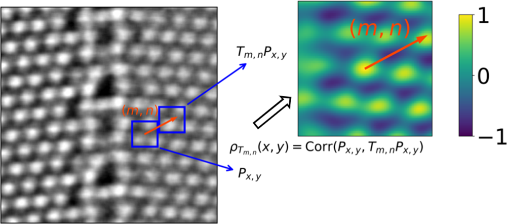
Fig. 3. Computing the local descriptors at pixel  $( x,\; y)$ based on translation operations. Left plot: an experimental HAADF-STEM image of two copper grains left and right separated here vertically by a grain boundary. Right plot: the calculated local-correlation map at pixel $( x,\; y)$.
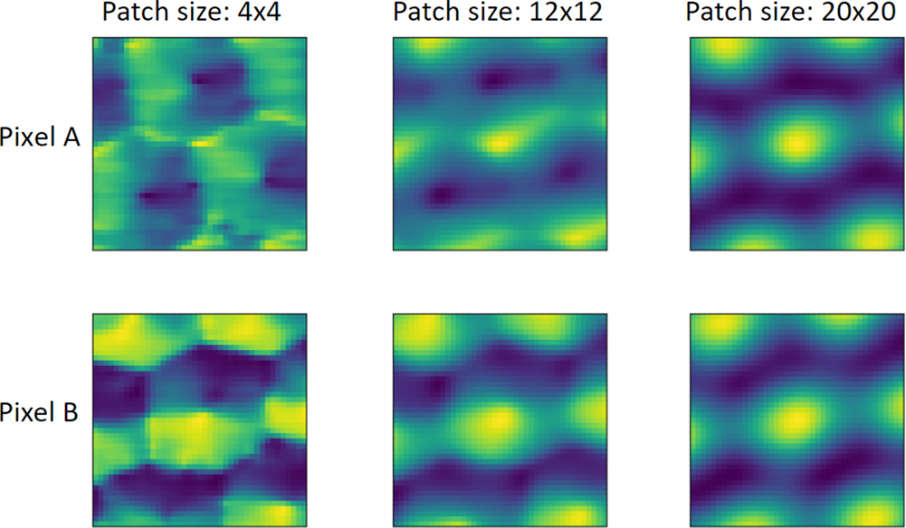
Fig. 4. Local-correlation maps of two selected pixels within the same crystal pattern in an HAADF-STEM image of size  $1,024\times 1,024$ pixels (shown in Fig. 10) evaluated with various patch sizes. The size of the local-correlation maps is $41\times 41$ pixels. The first (second) row are the local-correlation maps of pixel A (B). The first, second, and third columns are evaluated with square patch sizes of $4\times 4$, $12\times 12$, and $20\times 20$ pixels, respectively.
Before we move on to the discussion of the rotation/reflection-based local descriptors, it is worthwhile to first analyze what crystal patterns the translational-symmetry-based local descriptors are suitable to discriminate. Apparently, if the two crystal patterns have different Bravais lattices, lattice vectors, or orientations, we can employ the translational-symmetry-based local descriptors to discriminate them easily. But can the translation-symmetry-based local descriptors also discriminate crystal patterns that have the same Bravais lattice, lattice vectors and orientation and differ only in 2D plane group symmetries? As the entry in the local-correlation map is evaluated through the correlation coefficient between the original and the translationally shifted patch, the local-correlation map has the same symmetry as the auto-correlation function of the crystal pattern, the Patterson symmetry (Aroyo, Reference Aroyo2002).
The relationship between the 17 plane group symmetries and the 7 Patterson symmetries is presented in Table 1 (Aroyo, Reference Aroyo2002). The local-correlation map can only have seven Patterson symmetries because of extra constraints (Aroyo, Reference Aroyo2002). First, there is always a twofold rotational axis at the center, that is, the centrosymmetry. Second, the glide-reflection symmetry is not allowed and is replaced by the corresponding reflection symmetry. Clearly, if the two crystal patterns with the same lattice vectors and orientation have the same Patterson symmetry and different plane group symmetries, the translational-symmetry-based local descriptors cannot discriminate them. Thus, other types of symmetry operations need to be taken into account.
TABLE 1. The Seven Patterson Symmetries and the Plane Groups (Aroyo, Reference Aroyo2002).

Extracting Features via Rotation and Reflection Operations
Following the procedure shown in Figure 2, we present the implementation of the rotation-reflection-based local descriptors. In this case, it is more convenient to take circular patches and employ polar coordinates, interpolated from the original cartesian coordinates via cubic spline interpolation. The patches are rotated by a specific angle or reflected across a specific axis, and the symmetry score is again the Pearson's correlation coefficient between the original and the transformed patches, according to equation (2). We select a set of rotation angles  ${ 60^{\circ },\; 90^{\circ },\; 120^{\circ },\; 180^{\circ }}$ compatible with plane lattices, and also a set of reflection axes with different orientations. We then transform patches either by rotation around the central pixels or by reflections in the reflection axes through the central pixels. The symmetry score for each candidate symmetry operation represents a specific rotation or reflection symmetry feature. The local descriptors we obtain here cannot be used straightforwardly in the segmentation since they are not translationally invariant within the same crystal pattern. We present an example for a given reflection symmetry operation in Figure 5. The symmetry scores show clearly different preferences to the crystal patterns on the left- and right-hand sides. However, the symmetry scores are not homogeneously distributed within the crystal pattern indicating the point-group nature of the reflection and rotation symmetries. We add a max-pooling step to enforce the translational invariance, similar to the treatment in the convolutional neural networks (Boureau et al., Reference Boureau, Ponce and Lecun2010). As the max-pooling does not contain training parameters, our segmentation approach is still kept free of training.
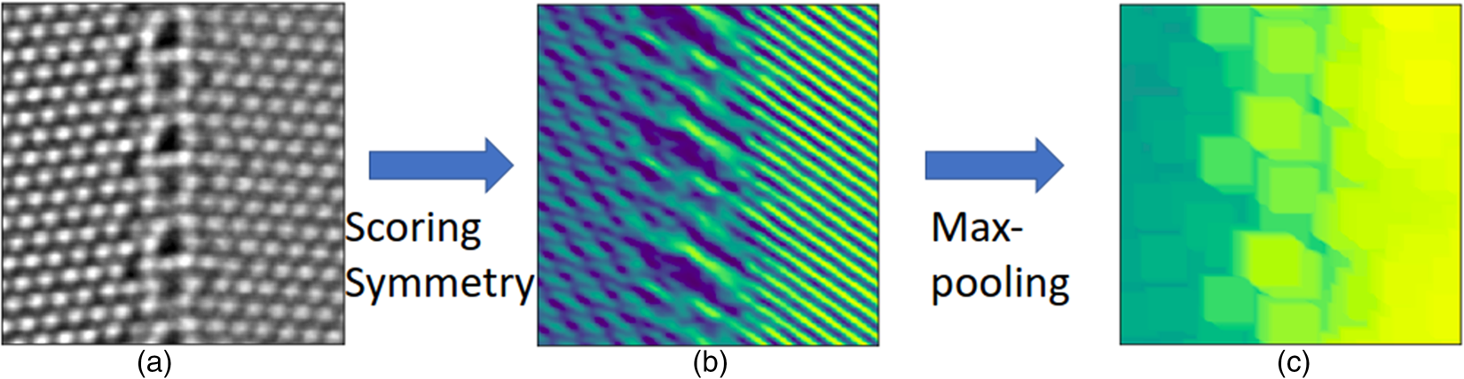
Fig. 5. An example to illustrate the calculation of reflection-based local descriptors. The rotation-based local descriptors can be obtained in a similar way. (a) An experimental HAADF-STEM image of two copper grains left and right separated vertically by a grain boundary. (b) The symmetry scores for a specific reflection symmetry operation at all pixels. The angle between the reflection axis and the horizontal line is 36 $^{\circ }$. The color coding represents values of reflection symmetry scores in the range $-$0.57 to 0.9. (c) The max-pooling enforces the translational invariance by only taking the largest elements in the pooling window. A pooling window of size $31\times 31$ pixels is used here.
Dimension Reduction
The local descriptor is a high-dimensional feature vector with each channel characterizing a specific symmetry. Only a few of these symmetries are relevant for distinguishing the crystal patterns present in the image. The other symmetry scores (in fact, the majority of entries) varies somewhat randomly across the image, and this random noise makes it difficult to discern different regions without an image-adapted metric, that would have high weights for relevant symmetries and low weights for the others. To circumvent this issue, it is advantageous to first reduce the dimensionality of the feature space.
We employ principal component analysis (PCA) for the dimension reduction. The implementation of PCA in scikit-learn (Pedregosa et al., Reference Pedregosa, Varoquaux, Gramfort, Michel, Thirion, Grisel, Blondel, Prettenhofer, Weiss, Dubourg, Vanderplas, Passos, Cournapeau, Brucher, Perrot and Duchesnay2011) is employed in our code. PCA provides an orthogonal basis in feature space, which diagonalizes the covariance matrix of the data set. As is common practice, we then choose those basis vectors that contribute most to the total variance. These optimal features are denoted PCA features. The number of PCA features is a parameter that can be either specified by users, or by requiring a lower bound for the so-called percentage of the variance explained, that is, the fraction of the total variance represented by the chosen PCA features. In Figure 6, we plot the percentage of variance explained (PVEn for the  $n$ most relevant features) versus the number $n$ of PCA features for the HAADF-STEM image shown in Figure 10 for different patch sizes. When the patch size is large enough, the first few PCA features are sufficient to capture the main variance of the image. We demonstrate below in the section “Application examples” that the dominant PCA features also have good separability to distinguish crystal patterns, making PCA suitable for dimension reduction in this work.
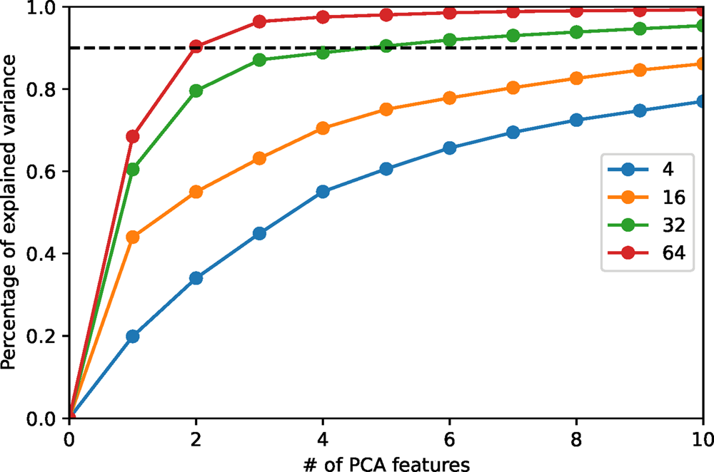
Fig. 6. The percentage of variance explained versus the number of PCA features for the HAADF-STEM image shown in Figure 10. The percentage of variance explained is evaluated via the ratio between the sum of variances of PCA features and that of raw features. Different colors represent different patch sizes. The black dashed line indicates 90% of total variance.
The correlation with the patch size is not surprising. We have shown above that the intrinsic uncorrelated noise of the image gives rise to noise in the symmetry scores, but averages out increasingly well as the patch size is increased. What we see in Figure 6 is therefore how the image noise carried over to the symmetry scores smears out relevant features over several components. Choosing the number of PCA features by a fixed threshold for the PVEn value, therefore, compensates to some extent the problem of choosing an optimal patch size and makes the overall procedure more robust. A suitable threshold depends on the image noise level and the number and fractions of distinct crystalline phases in the image. A threshold value of 80–90% is recommended based on our experience.
K-Means Clustering
We feed the PCA features into the k-means clustering algorithm (MacQueen, Reference MacQueen1967; Arthur & Vassilvitskii, Reference Arthur and Vassilvitskii2007) to cluster the pixels in the feature space. This algorithm finds the cluster centers by minimizing the within-cluster sum of squares criterion that measures the internal variability of clusters. Each cluster corresponds to a specific crystal pattern, and the pixels grouped into the same cluster are assigned with the same pattern label. Once the cluster centers are found, we partition the feature space into Voronoi cells. We employ the implementation of k-means clustering in scikit-learn (Pedregosa et al., Reference Pedregosa, Varoquaux, Gramfort, Michel, Thirion, Grisel, Blondel, Prettenhofer, Weiss, Dubourg, Vanderplas, Passos, Cournapeau, Brucher, Perrot and Duchesnay2011) in our code. The cluster centers are first initialized randomly and then optimized in an iterative way. The number of clusters is one hyperparameter that needs to be specified by the users. It means that users need to specify the number of crystal patterns into which they want to partition an image.
Once the relevant crystal patterns have been identified, they can be used to construct a “fast” classifier based on only those symmetries that are actually most relevant to the crystal patterns in the image. This might be particularly useful for image series and videos, as one restricts the computationally intense brute-force extraction of crystal pattern classifiers to a few representative frames, and then uses the symmetry-selective classifier for the full segmentation. This consideration leads us to develop a separability-analysis scheme for efficient segmentation of image series and videos.
Speedup for Image Series: Separability Analysis
We employ a separability-analysis scheme to reduce the computational cost for segmentation of a large number of images with similar features, for example, in situ videos. The separability-analysis scheme selects the symmetry operations that are most relevant to the crystal patterns in the image. The selected symmetry operations can then be used to segment other images with similar features. The computational cost is reduced drastically as much fewer symmetry operations are used to segment these images. In practice, we first perform a segmentation of a representative image, which might be the first frame of a video. A large number of symmetry operations is required in this step, as we do not know beforehand which symmetry operation is crucial for the segmentation. After that, we calculate the Fisher's separability (Fisher, Reference Fisher1936) for each symmetry operation. For a given symmetry operation  $O$, its Fisher's separability is defined by
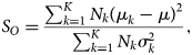 $$S_O = {\sum_{k = 1}^{K} N_k( \mu_k-\mu) ^{2}\over \sum_{k = 1}^{K} N_k \sigma_k^{2} },$$ $K$ is the total number of patterns (classes). $\mu _k$ and $\mu$ are the within-class mean and the total mean of the symmetry feature generated by the given symmetry operation $O$.
$O$.  $\sigma _k^{2}$ is the within-class variance. The separability indicates how well the symmetry operation $O$ can discriminate the crystal patterns. We then use Fisher's separability to select a small number of symmetry operations for segmentation of all other images.
To explore the potential benefit of this optimization, we performed a time cost and accuracy test with an HAADF-STEM video of 163 frames. The results are shown in Figure 7. We first perform a segmentation on the first frame with 289 translational operations. With the pattern labels obtained from this segmentation, we perform a separability analysis and calculate each translational operation's separability. We then select  $n$ translational operations with the best separability and measure the time cost and accuracy of the segmentation with them. $n$ is chosen to be 2, 50, 100, 150, 200, and 289 in this test, and the accuracy is calculated relative to the segmentation result with 289 translational operations. We see a linear decrease of the time cost with the decreasing number of translational operations, whereas the accuracy is always over 95%.
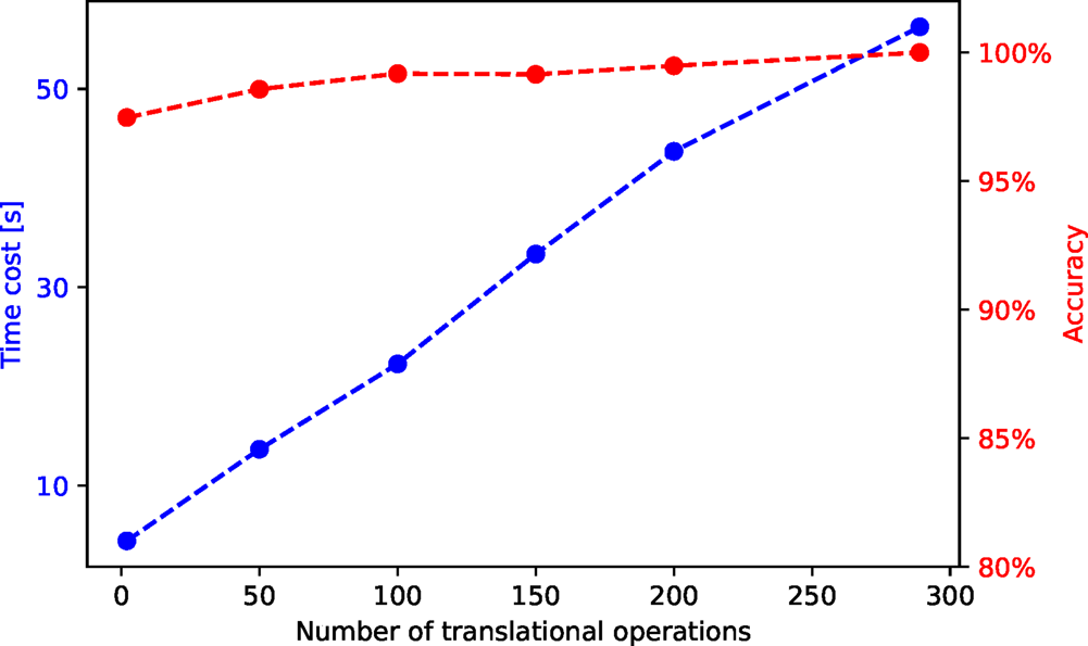
Fig. 7. Time cost and accuracy for segmentation of an HAADF-STEM video with 163 frames and different numbers of post-selected translational operations. The raw and segmented videos are shown in the Supplementary material.
Application Examples
In Figure 8, we present an application to the HAADF-STEM image containing two phases ( $\mu$ phase and Laves phase) of the iron–niobium intermetallic compound. More experimental details can be found in Šlapáková et al. (Reference Šlapáková, Zendegani, Liebscher, Hickel, Neugebauer, Hammerschmidt, Ormeci, Grin, Dehm, Kumar and Stein2020). The pattern labels are correctly assigned to the pixels in the two phases, as shown in Figure 8.
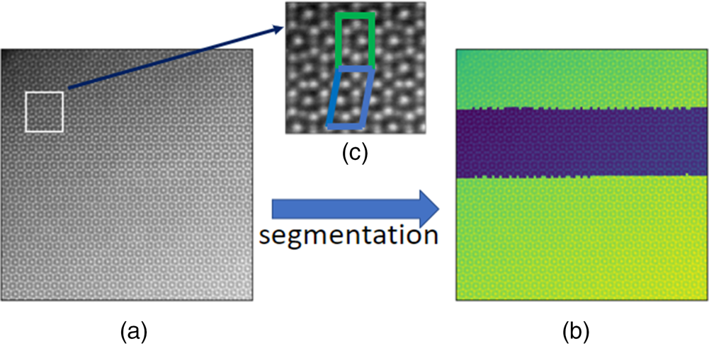
Fig. 8. (a) An HAADF-STEM image of size  $1,024\times 1,024$ pixels containing two phases ( $\mu$ phase and Laves phase) of the iron–niobium intermetallic compound. The pixel size is $0.125\times 0.125$ Å. (b) The image superimposed of the HAADF intensity and the pattern labels. (c) The zoomed plot of the white window. The repeating units of the two phases are marked in green and blue.
This example nicely illustrates why our segmentation approach works in an unsupervised manner. To show this, we calculate the Fisher's separability (Fisher, Reference Fisher1936) and variances for all features in the local descriptors and the five PCA features with largest variances. In Figure 9, we see a strong correlation between separability and variance. A feature that has a larger variance also has a better separability. We might think of features with good separability as the signal and those with bad separability as the noise. The correlation between separability and variance is crucial for the unsupervised approach, which results in a good signal-to-noise ratio and ultimately successful segmentation.
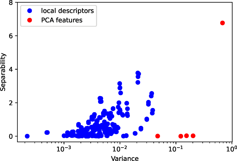
Fig. 9. The separability and variance of all features in the local descriptors and the five PCA features.
The second example is shown in Figure 10. In this example, we segment an HAADF-STEM image containing two differently oriented copper crystals separated vertically by one tilt grain boundary with the reflection- and rotation-symmetry-based local descriptors, separately. The reflection-symmetry-based local descriptors successfully partition the image into the left (green) and right (violet) crystal, but are not capable of identifying the grain boundary as seen in Figure 10b. This is because the reflection symmetries are sensitive to the local crystal orientation. The rotation-symmetry-based local descriptors group the two grains into the same crystal pattern (green) as shown in Figure 10c and segment the grain boundary region (violet) based on its different rotational symmetry. The results emphasize the influence of the choice of local descriptors, since they capture different symmetry information. In this example, the reflection-symmetry-based local descriptors are not rotationally invariant, and therefore, both disoriented crystals are partitioned into different crystal patterns. In contrast, the rotation-symmetry-based local descriptors are rotationally invariant and result in different interpretation of the crystal patterns in the image.
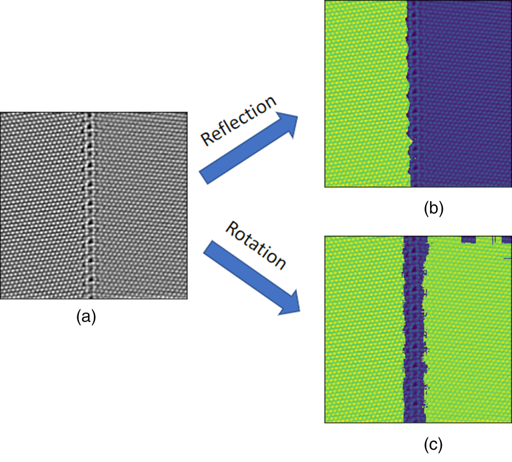
Fig. 10. (a) An HAADF-STEM image of size  $1,024\times 1,024$ pixels containing two Cu single-crystal grains and a tilt grain boundary. The pixel size is $0.0623\times 0.0623$ Å. (b) Segmentation via the reflection-based local descriptors. The image is superimposed of the HAADF intensity and the class labels. (c) Segmentation via the rotation-based local descriptors. The image is superimposed of the HAADF intensity and the pattern labels.
In our third example shown in Figure 11, we segment the HAADF-STEM image of Pd nanocrystals obtained from electrochemical etching of a PdCoO $_2$ single crystal (Podjaski et al., Reference Podjaski, Weber, Zhang, Diehl, Eger, Duppel, Alarcón-Lladó, Richter, Haase, i Morral, Scheu and Lotsch2019). These nanocrystals have two twin variants and many free volumes (holes) in between. The image has, therefore, significant variations in the overall intensity (mass-thickness contrast of HAADF), from zero-thickness in the hole, single nanograin to multiple grains stacked along the projection. Nevertheless, we observe that the segmentation using the local-correlation map descriptor retains a very good spatial resolution, correctly identifies the twin phases (yellow, blue), and makes them readily visible in the segmented image in comparison to the original one. Furthermore, we added in a third pattern (red), and the algorithm assigns it to the hole and some strongly blurred regions that are essentially structureless, demonstrating that the algorithm can deal with image parts without a crystalline structure.
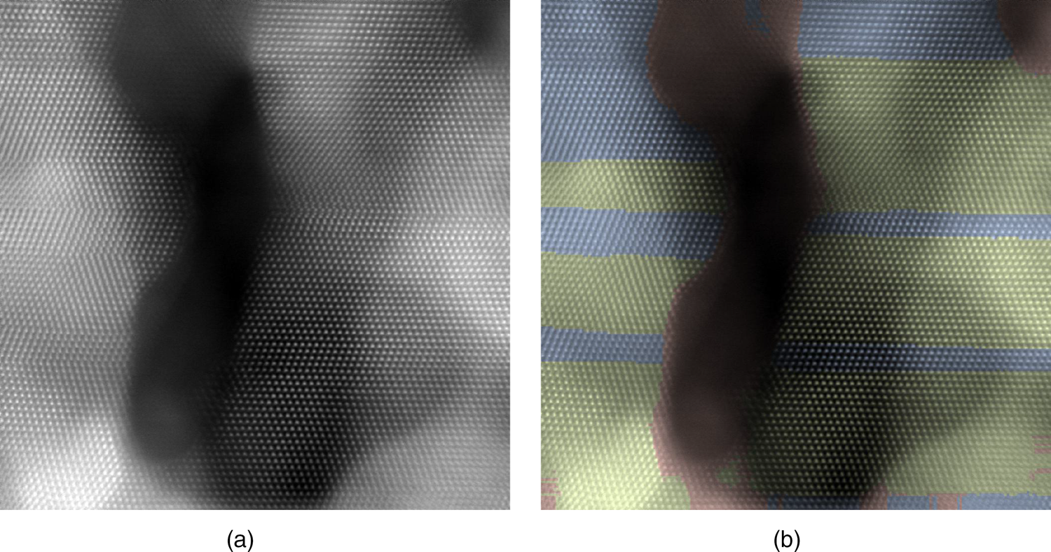
Fig. 11. (a) An HAADF STEM image of size  $1,024\times 1,024$ pixels containing palladium nanocrystals with surfaces and twin boundaries. The pixel size is $0.1761\times 0.1761$ Å. (b) The segmentation via the translation descriptors is shown by colors (yellow/blue/red).
In a fourth example, we demonstrate that our unsupervised segmentation can also be applied to atomic-resolution TEM videos obtained from in situ heating experiments. The video sequence shows the temperature-induced de-twinning process in an FeMnCoCrNiC-based high entropy alloy obtained at 900 $^{\circ }$C. The raw video and segmented video are presented in the Supplementary material. Without prior knowledge in the structure present in the image, the unsupervised segmentation is able to identify the matrix and twin regions, which is the basis for a complete quantitative analysis of the data set. From the segmented data, important information such as the de-twinning speed and migration dynamics of the incoherent twin boundary can be inferred with little effort after segmentation using feature tracking.
We provide the jupyter notebooks for the calculations in this section (Wang, Reference Wang2021c), and all the figures might be reproduced with little effort.
Conclusion
We present an unsupervised machine-learning approach to segment atomic-resolution microscopy images without prior knowledge of the underlying crystal structure. In our approach, we extract a local descriptor through scoring candidate symmetry operations by the Pearson's correlation coefficient, which forms an abundance feature vector to characterize the local symmetry information. We then use PCA to reduce the dimension of the local descriptors. After that, we feed the PCA features into a k-means clustering algorithm in order to assign pattern labels to pixels. To reduce computational cost, a stride and upsampling scheme is proposed. A separability-analysis step is added in order to segment image series or video sequences efficiently. We present the successful application to experimental HAADF-STEM images, image series, and high-resolution TEM videos, and reveal one important feature of the unsupervised segmentation approach, the strong correlation between the feature's separability and variance. We package our code as a python module, and release it in the github (Wang, Reference Wang2021c), conda-forge (Wang, Reference Wang2021b), and the python package index repository (Wang, Reference Wang2021a). More tests can be found in the example folder in our github repository.
Supplementary material
To view supplementary material for this article, please visit https://doi.org/10.1017/S1431927621012770.
Acknowledgments
The authors gratefully acknowledge funding from BiGmax Network. Dr. Wenjun Lu at MPIE is gratefully acknowledged for providing the HAADF-STEM video shown in the Supplementary material.
Appendix A. Summary of Hyperparameters
We summarize the hyperparameters in our workflow.
1. descriptor_name. It is used to select the type of local descriptors. We have implemented five types of descriptors till now. The default is local-correlation-map.
(a) local-correlation-map. The translational-symmetry-based local descriptor in subsection “Extracting Features via Translation Operations” are used for segmentation. The translational operations are chosen uniformly from a window.
(b) preselected_translations. The translational-symmetry-based local descriptors in subsection “Extracting Features via Translation Operations” are used for segmentation. Different from local-correlation-map, the translational operations are provided by users explicitly.
(c) rotational_symmetry_maximum_pooling, the rotational-symmetry-based local descriptors with maximum pooling discussed in subsection “Extracting Features via Rotation and Reflection Operations.”
(d) reflection_symmetry_maximum_pooling. The reflectional-symmetry-based local descriptors with maximum pooling discussed in subsection “Extracting Features via Rotation and Reflection Operations.”
(e) power_spectrum, absolute values of discrete Fourier transform (Borodinov et al., Reference Borodinov, Tsai, Korolkov, Balke, Kalinin and Ovchinnikova2020; Jany et al., Reference Jany, Janas and Krok2020).
2. For each type of the local descriptors above, we need some hyperparameters to specify the implementation details. We list all the relevant hyperparameters below.
(a) local-correlation-map.
• patch_x. The half height of rectangular patches that are translated to calculate translational-symmetry-based local descriptors, corresponding to $p_x$ in subsection “Extracting Features via Translation Operations.”
• patch_y. The half width of rectangular patches corresponding to
$p_y$, corresponding to $p_y$ in subsection “Extracting Features via Translation Operations.”• window_x. The half height of the rectangular shift window that confine translation shifts corresponding to
$w_x$ in subsection “Extracting Features via Translation Operations.”• window_y. The half width of the rectangular shift window that confine translation shifts corresponding to
$w_y$ in subsection “Extracting Features via Translation Operations.”• max_num_points. The maximum number of translation operations to choose from the shift window. There are
$( 2\ast w_x + 1) \ast ( 2\ast w_y + 1)$ translation operations in the shift window. Instead of using all the translation operations, we setup a uniform grid in the shift window and only use the grid points to choose the translation operations. We build the uniform grid as dense as possible, and the number of grid points are not larger than max_num_points.• method. This parameter is used to select the method to compute local descriptors, which can be “direct” or “fft.” The default is “direct.” We implemented two methods to calculate local-correlation map, the direct method and the method based on fast Fourier transform.
(b) preselected_translations.
• patch_x. Its syntax has been explained above.
• patch_y. Its syntax has been explained above.
• preselected_translations, which is a 2D numpy array. Each row specifies a translational vector.
(c) rotational_symmetry_maximum_pooling.
• radius. The radius of the circular patch.
• window_x. The half height of the rectangular window for max pooling.
• window_y. The half weight of the rectangular window for max pooling.
(d) reflection_symmetry_maximum_pooling.
• radius. Its syntax has been explained above.
• num_reflection_plane. The number of reflection planes corresponding to the number of reflection-symmetry-based features.
3. n_patterns. The number of patterns to partition the image into. It corresponds to the number of clusters in K-means clustering. The default is 2.
4. upsampling. A Boolean parameter. If True, the upsampling is performed on the output label array to match the size of input image. The default is True.
5. stride. The stride size for both vertical and horizontal directions.
6. separability_analysis. A Boolean parameter. If True, the separability analysis is performed for each feature. The default is False.
7. random_state. It can be an integer value or None. The random number generation is required in the centriod initialization in the K-means clustering. We may set this parameter to an integer value for reproducibility. The default is None.
8. sort_labels_by_pattern_size. A Boolean parameter. If True, sort the pattern labels by size of patterns. The smallest pattern has a label of 0, and the largest pattern has a label of n_patterns-1. The default is True.


Appendix B. FFT Implementation of Translational-Symmetry-Based Local Descriptors
The numerator of Pearson's correlation coefficient for translation  $T_{m, n}$ can be rewritten as
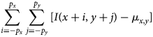 $$\sum_{i = -p_x}^{\,p_x}\sum_{\,j = -p_y}^{\,p_y} [ I( x + i,\; y + j) - \mu_{x, y}] $$
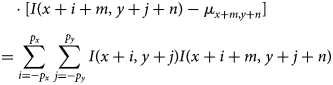 $$\eqalign{& \qquad \cdot [ I( x + i + m,\; y + j + n) - \mu_{x + m, y + n}] \cr & \quad = \sum_{i = -p_x}^{\,p_x}\sum_{\,j = -p_y}^{\,p_y} I( x + i,\; y + j) I( x + i + m,\; y + j + n) }$$
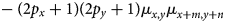 $$\qquad - ( 2p_x + 1) ( 2p_y + 1) \mu_{x, y}\mu_{x + m, y + n}$$
where  $I( \cdots )$ denotes the pixel values of the entire image, and
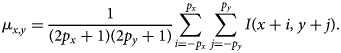 $$\mu_{x, y} = {1\over ( 2p_x + 1) ( 2p_y + 1) } \sum_{i = -p_x}^{\,p_x}\sum_{\,j = -p_y}^{\,p_y} I( x + i,\; y + j) .$$
Similarly, the norm of the displaced patch in the denominator can be written as
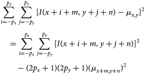 $$\eqalign{& \sum_{i = -p_x}^{\,p_x}\sum_{\,j = -p_y}^{\,p_y} [ I( x + i + m,\; y + j + n) - \mu_{x, y}] ^{2}\cr & \quad = \sum_{i = -p_x}^{\,p_x}\sum_{\,j = -p_y}^{\,p_y} [ I( x + i + m,\; y + j + n) ] ^{2}\cr & \qquad - ( 2p_x + 1) ( 2p_y + 1) ( \mu_{x + m, y + n}) ^{2}}$$
The norm of the undisplaced patch corresponds to the special case  $m = n = 0$.
The sums appearing in the equations (B.3)–(B.5) for all translations  $( m,\; n)$ with $-w_x \le m \le w_x$ and $-w_y \le n \le w_y$ can be computed efficiently via fast Fourier transforms (FFTs). For this, we note that the sums can be brought to a common form
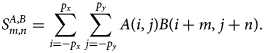 $$S^{A, B}_{m, n} = \sum_{i = -p_x}^{\,p_x}\sum_{\,j = -p_y}^{\,p_y} A( i,\; j) B( i + m,\; j + n) .$$ $A( i,\; j)$ is required for a range $( -p_x\dots p_x) \times ( -p_y \dots p_y)$ and $ ( i' = i + m,\; j' =$ $B j + n)$ for a larger range $( -p_x-w_x) \dots p_x + w_x) \times ( -p_y-w_y \dots p_y + w_y)$. For the sum in equation (B.3), $A( i,\; j) = I( x + i,\; y + j)$ and $ B( i',\; j') =$ $ I( x + i',\; y + j') $. For equations (B.4) and (B.5), $A( i,\; j) = 1$ in both cases, while $B( i',\; j') = I( x + i',\; y + j')$ for the mean and $B( i',\; j') = [ I( x + i', $ $ y + j') ] ^{2} $ for the norm.
We now embed  $A$ and $B$ in an extended range $( 0 \ldots W_x-1) \times ( 0 \ldots$
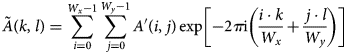
  $ W_y-1)$ using periodic boundary conditions and zero-padding, see Figure B.1. We are free to choose optimal $W_x$ and $W_y$ satisfying $W_x \ge 2( w_x + p_x) + 1$ and $W_y \ge 2( w_y + p_y) + 1$. This means that originally positive indices $i,\; j$ (including zero) are left unchanged, negative ones are mapped to $W_x + i$ and $W_x + j$, respectively, and the values not covered by the original ranges are set to zero. We denote the mapped quantities with $A'$ and $B'$. The sums in equation (B.6) can then be extended to cover the full range,
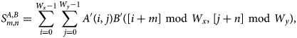 $$S^{A, B}_{m, n} = \sum_{i = 0}^{W_x-1}\sum_{\,j = 0}^{W_y-1} A'( i,\; j) B'( [ i + m] \ {\rm mod}\ W_x,\; [ j + n] \ {\rm mod}\ W_y) ,\; $$
which, in turn, is easily recognized as a periodic convolution. Using the Fourier theorem, the convolution can be obtained from a forward discrete Fourier transform
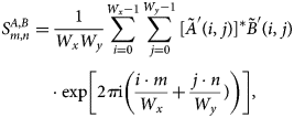 $$\eqalign{S^{A, B}_{m, n}& = {1\over W_xW_y}\sum_{i = 0}^{W_x-1}\sum_{\,j = 0}^{W_y-1}[ \tilde A'( i,\; j) ] ^{\ast } \tilde B'( i,\; j) \cr & \quad \cdot \exp\left[2\pi {\rm i} \left({i\cdot m\over W_x} + {\,j\cdot n\over W_y}) \right)\right],\; }$$
where the complex-valued quantity
 $$\tilde A( k,\; l) = \sum_{i = 0}^{W_x-1}\sum_{\,j = 0}^{W_y-1} A'( i,\; j) \exp\left[-2\pi {\rm i} \left({i\cdot k\over W_x} + {\,j\cdot l\over W_y}\right)\right]$$
is obtained from an inverse discrete Fourier transform.  $\tilde B'$ is obtained analogously. The forward and inverse discrete Fourier transforms can be computed using FFT algorithms with an effort ${\cal O}( W_xW_y \ln [ W_xW_y] )$. This can be contrasted to the straightforward algorithm with an effort of $( 2 w_x + 1) ( 2w_y + 1) $ $( 2p_x + 1) ( 2p_y + 1) \approx {1 \over 4} ( W_xW_y) ^{2}$ if $w_x\approx p_x$ and $w_y \approx p_y$. For computing the three sums in equations (B.3)–(B.5), one needs four inverse transforms, and three forward transforms. Additional savings could be made by precalculating the patch norms for the entire image rather than for each patch center $x,\; y$ in the required environment, and by precalculating the inverse transform for the case $A( i,\; j) = 1$ once for all patch centers, reducing the subsequent effort to 4 FFTs per patch center.
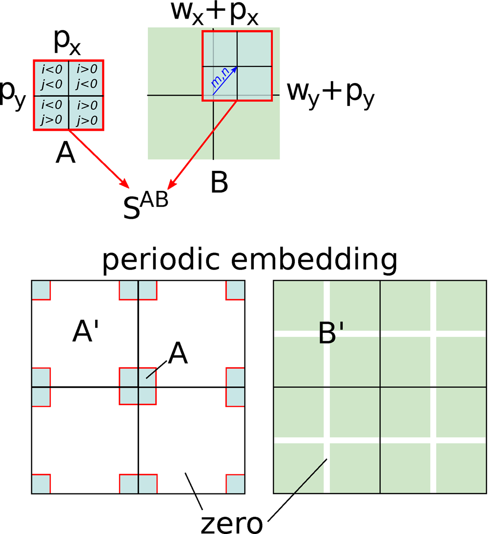
Fig. B.1. Sketch of the FFT algorithm for shifted summation. After embedding  $A$ and $B$ in a sufficiently large periodic range with zero-padding, the shifted summation becomes a periodic convolution in the extended range. Periodicity is indicated by showing a $2\times 2$ repetition.
Appendix C. Speedup Scheme for Single Images/Frames: Stride and Upsampling
We employ a stride and upsampling scheme to reduce computational cost. Stride means we only calculate local descriptors for a fraction of pixels, that is, the image is downsampled. The upsampling scheme is then employed to estimate pattern labels of the pixels whose local descriptors are not evaluated. To assign a pattern label for each pixel, a straightforward approach would require to calculate local descriptors and perform clustering for all pixels, for example, around one million pixels for a  $1,024\times 1,024$ image. Alternatively, we may first use the stride scheme to downsample the image, and then perform upsampling after the clustering is finished in order to match the size of the original image. In this way, we can reduce the computational cost drastically. The stride scheme we employ is identical to the one used in convolutional neural networks. To be more specific, in the first step of our approach, instead of calculating the local descriptors for each pixel by shifting the local-symmetry-feature extractors every time by one unit, we shift them by a step size of $s$ units vertically and horizontally and only calculate the local descriptors for a fraction of pixels. The selected pixels in the stride step will obtain pattern labels from the k-means clustering whereas those unselected ones will not. To assign pattern labels to the unselected ones, we simply do a nearest neighbor interpolation in our upsampling step, that is, the unselected pixels obtain pattern labels identical to the selected pixels that are closest to them. In the end, we obtain a segmented image that has the same size as the original one. The upsampling scheme contains no training parameters, which keeps our whole approach free of training.
In Figure C.1, we show a time cost and accuracy test for the stride and upsampling scheme. The purpose is not to provide an absolute timing benchmark, but to illustrate the tuning opportunities inherent to this scheme. For this test, we use an HAADF-STEM image of size  $1,024\times 1,024$ pixels. The time cost decreases roughly with $1/{\rm stride}^{2}$ whereas the accuracy keeps above 97% for all the strides in this test.
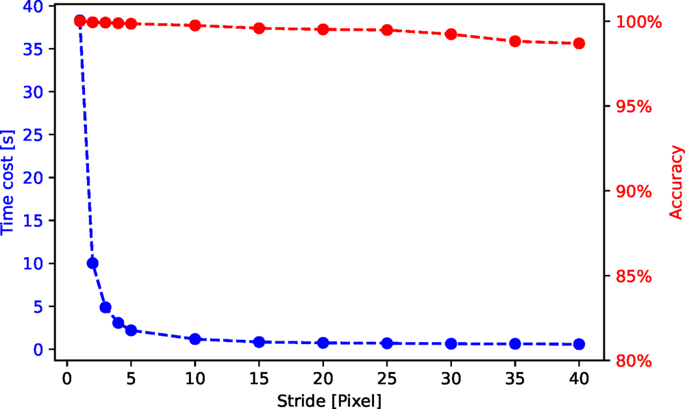
Fig. C.1. Time cost and accuracy for segmentation of an HAADF-STEM image (shown in Fig. 10) with different strides.


 Open access