


1. Introduction
Cold ice sheets with temperatures below pressure-melting point and negligible amounts of meltwater (not affecting the ice flow) are distinguished from usually smaller and temperate ice caps (temperatures at pressure-melting point) where meltwater is present within the ice body (Reference PatersonPaterson, 1994).
An example of the latter are the ice caps of the sub-Antarctic islands which have been subject to increasing surface temperatures over the last few decades (Reference TurnerTurner and others, 2005). King George Island (KGI), the largest of the South Shetland Islands, is located in the marginal sea-ice zone north of the Antarctic Peninsula at 62˚S, 58 ˚W and is influenced by subpolar maritime climate conditions (Fig. 1).
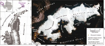
Fig. 1. Location of King George Island. Left: map prepared from Antarctic Digital Database (ADD) and RADARSAT Antarctic Mapping Project (RAMP) data; right: courtesy of SPOT Image 1995/2000.
The high number of permanent research stations and a gravel runway on the ice-free Fildes Peninsula reflect the good accessibility of KGI, making it an ideal place to study the effects of atmospheric warming on small ice caps within a maritime climate. Reference Wen, Kang, Han, Xie, Liu and WangWen and others (1998) state that the mean annual temperature at sea level is –2.4˚C, that the firn is temperate at altitudes above 380 m and that substantial percolation takes place in the firn forming ice lenses (see also Reference SimõesSimões and others, 2004).
Reference Simões, Bremer, Aquino and FerronSimões and others (1999) identify 70 drainage basins in the 1250 km2 KGI ice cap where several southeast ice fronts have retreated rapidly since the late 1950s, some by more than 1 km. Despite the ideal logistical situation of KGI, little research has been carried out regarding determination of ice thickness and the geometries of surface and bedrock. Previous radio-echo sounding was restricted to a narrow corridor from Bellingshausen Dome along the main ice divide to the Main Dome. The results were ambiguous and suffered from absorption and scattering (Reference Govorukha, Chudakov and ShalyginGovorukha and others, 1975; Reference Simões and BremerSimões and Bremer, 1995; Reference Macheret and MoskalevskyMacheret and Moskalevsky, 1999; Reference Travassos and SimoesTravassos and Simões, 2004).
Data used for this paper were collected during a Brazilian–German expedition in 1997/98 by teams from the University of Münster (UM), the University of Freiburg (UF) and NUPAC (Nucléo de Pesquisas Antárticas e Climáticas) in 1999/2000 and by UM and the University of Bonn (UB) in 2004/05. The investigated area was extended in 2007 by a German expedition from UM and UB with the aim of completing the geometry and surface movement data (for the latter see Reference Rückamp, Blindow, Suckro, Braun and HumbertRückamp and others, 2010).
The investigated area, campsites, locations and profile lines are shown in Figure 2. Results from single-location surface energy-balance computations based on readings from automatic weather stations (AWSs) located in different altitudes in the study area are given by Reference Braun, Saurer, Vogt, Simões and GossmannBraun and others (2001, Reference Braun, Saurer and Gossmann2004).

Fig. 2. GPR profiles, locations of camps and common midpoints (CMPs) in the 1997 and 2007 field campaigns. Background image: SPOT satellite image mosaic (courtesy of Eurimage 1995/2000).
Spatially distributed melt modelling was carried out based on the 1997/98 AWS dataset by Reference Braun and HockBraun and Hock (2004). The results showed the impact of the distinct atmospheric circulation patterns on melt rates. Considerable surface melt was observed and modelled for December January of 1997/98 and 1999/2000 up to the highest elevations of the KGI ice cap. A firn profile at about 619ma.s.l. instrumented with thermistor strings in 1999/2000 showed a 10m firn temperature of about –0.3°C. The winter cold content of the surface snowpack, still observable in early December, was continuously filled by percolating meltwater during subsequent weeks.
Since the melt period of KGI extends into March/April, considerable meltwater percolation, even to deeper layers of the snowpack, has to be expected. This confirms the findings of a water table and the problems of water intrusion in the borehole of an earlier ice-coring attempt in 1995/96 (Reference SimõesSimoes and others, 2004) at 62°07’S, 58°37’W (690 ma.s.l.). Reference SimõesSimoes and others (2004) also reported a snow-ice transition at 35 m and a borehole temperature of –0.35 to –0.25˚C at 45 m depth, still slightly below pressure-melting point.
Helicopter-borne measurements to cover the crevassed areas were planned during several seasons, but could only be accomplished in the austral summer of 2009 and cannot yet be integrated here.
We provide a summary of the results of ground-penetrating radar (GPR) and differential global positioning system (DGPS) measurements of the geometry, internal structures and thermal regime of the KGI ice cap.
2. Instruments
2.1. Choice of GPR centre frequency
Temperate ice usually contains inhomogeneities such as water pockets and ducts which may cause heavy scattering of electromagnetic waves of comparable wavelengths (Rayleigh and Mie scattering). Normally this is overcome by utilizing low-frequency radars (of a few megahertz with wavelengths in ice of up to 100 m) which usually suppress scattering effects and show a distinct bedrock reflection.
Scattered energy can be focused by geophysical data processing, namely the process of migration. This technique was developed to process reflected seismic data. Lateral and vertical resolution may be increased significantly and scattering effects are compressed. Reference Blindow and ThyssenBlindow and Thyssen (1986) carried out the first successful soundings of temperate ice at 30 MHz centre frequency (wavelength in ice is 6 m), with subsequent computerized migration as a processing tool.
2.2. Field campaign, 1997
The GPR equipment used was the Münster monopulse GPR system as described by Reference BlindowBlindow (1994). A major change was applied with respect to the antenna system: it utilized a shielded broadband antenna with 50 MHz centre frequency similar to the design discussed in Reference Eibert, Hansen, Blindow and SteinEibert and others (1997).
The DGPS equipment consisted of four Magellan ProMark X-CM receivers. The same models were used for the 2004/05 measurements.
2.3. Field campaign, 2007
The GPR equipment comprised a commercial SIR-3000 console with a DA769 receiving unit of Geophysical Survey Systems Inc. (GSSI) and a 1 kV metal-oxide semiconductor field-effect transmitter (MOSFET) triggered via a fibre-optic link (constructed by the University of Münster). The antennae with a centre frequency of 25 MHz were combinations of folded broadband dipoles (Reference Peters, Young and MillerPeters and Young, 1986) and resistively loaded dipoles (Reference Wu and KingWu and King, 1965).
The DGPS equipment consisted of four dual frequency receivers in two pairs of NovAtel DL4 and Trimble 4000 SSE. The set-up used in the field is shown in Figure 3.

Fig. 3. The GPR antennae and a sledge with the GPR control unit are dragged by a snowmobile with a DGPS system.
3. GPR Measurements
3.1. CMP measurements
In both field campaigns, common-midpoint (CMP) measurements were performed to determine the velocities of the radar signals in the subsurface. The locations of the CMPs are depicted in Figure 2; the 1997 CMP was located 607 m a.s.l. and the 2007 CMP at 620 m a.s.l. Figure 4 depicts the velocity adaption of a three-layer model to the 2007 data as determined with the ReflexW program (K.J. Sandmeier software). Hyperbola reflections are caused by the water table, isochrones and the bedrock. The 1997 data resulted in a two-layer model based on the water table and bedrock reflections.

Fig. 4. CMP analysis: velocity–depth model and processed data.
The models are very similar, with average velocities in the firn layer of 0.194 and 0.193 m ns−1 . In the two-layer model, a velocity of 0.168 m n s−1 is proposed for the ice between the water table and bedrock. The three-layer model has an additional layer with 0.175 m n s−1 between the water table and 80 m depth, until reaching 0.168 m ns−1. The variability of firn thickness with altitude introduces uncertainty in the estimated velocities, and we estimate the best accuracy to be ±1.7%.
3.2. GPR profiles
The radar data were processed in several steps (at 25 MHz centre frequency) comprising a time-zero correction corresponding to the antenna offset, a frequency domain bandpass filter from 17 to 80 MHz and a despiking filter. The direct signal was reduced to enhance the water table reflection. Time-domain migration (diffraction stack) with a single velocity was used to collapse diffraction hyperbolas and to recover the actual dip of reflectors (which is true only in the case of a two-dimensional (2-D) geometry or point diffractors). Finally, to account for dielectric losses in the temperate ice, a gain of 0.08 dB m−1 was applied.
A typical example of the processed radar data obtained near the ice divide can be seen in Figure 5. For easier interpretation, the profile is vertically exaggerated and topographically corrected. A strong reflection marks the water table at an average depth of 35 m, which indicates the firn–ice boundary. Layering inside the ice is visible by isochrones, which are arching up near the ice divide. These arches are patterns of ice dynamics called Raymond bumps (Reference RaymondRaymond, 1983). The irregular reflections at the bottom of the radargram are caused by the ice–bedrock interface.

Fig. 5. Typical radargram near the ice divide showing a water table at 600–650 m a.s.l., bedrock in red at 300–500 ma.s.l. and uparching of isochrones starting at 550 m a.s.l. (right-hand side).
3.3. Thermal regime from interpretation of GPR data
The spatial distribution of internal features was studied in detail using the 1997/98 dataset. The results can also be extrapolated and verified in other parts of the KGI ice cap. Water inclusions are seen in the radargrams as small hyperbolic diffraction features. Some single-point diffractors, possibly caused by water-filled ducts or voids, and a strong reflection of the water table are present almost throughout the ice cap. Diffraction features are abundant in areas of surface elevation below 400 m a.s.l. but are scarce or absent in areas above that. We used the abundance of diffractions (high backscatter) as an indication for temperate ice caused by liquid water content. This method of discriminating cold and temperate ice in alpine glaciers was also used by Reference Eisen, Bauder, Lüthi, Riesen and FunkEisen and others (2009).
It is noted that radar backscatter vanishes on the few profiles below the equilibrium line (at 160 m a.s.l. in 1991/92) which are cold according to Reference Wen, Kang, Han, Xie, Liu and WangWen and others (1998).
4. Topographical Results
Surface and bedrock topographies were generated by merging the datasets. The coastline was added with values of 0 m for the surface elevation, and ice-thickness and bedrock elevation data were also combined.
The accuracy of surface topography is estimated from the GPS accuracies. The vertical accuracy of single-frequency DGPS in kinematic mode is 1.6 m and a few centimetres in static mode. The vertical accuracy of dual-frequency systems is usually in the centimetre range. Due to vertical displacements of the base station and other effects, we estimate a vertical error of 0.2 m for kinematic measurements. Ice-thickness accuracy varies from about 2 m in areas with a smooth bed to about 10 m in areas with a rough or undulating bed.
These topography data were gridded with Surfer (Golden Software, Inc.), using the kriging algorithm on a 500 m grid. To include the area between the outer profiles and the coast, the radius for kriging was set to 10 km. To smooth the contours, two nodes were inserted between the lines by the spline smooth function.
4.1. Ice thickness map
Figure 6 shows the ice thickness in the surveyed area without the interpolated margins. The mean ice thickness along the profiles is 250 m, with a maximum of 422 m in the eastern part of the central ice cap. Some southeast–northwest areas of thick ice indicate the main drainage valleys of the ice cap. This can also be seen in the bedrock topography as described in section 4.2.
Fig. 6. Ice thickness in the surveyed area on KGI.
4.2. Surface and bedrock topography
Three-dimensional (3-D) models of the surface and bedrock topography are depicted in Figure 7. These were generated as described previously, including the interpolated margin between the GPR profiles and the coastline. The surface of the ice cap rises slowly from the northwest coast to the ice divide, while the southeast slope is much steeper. Two main domes dominate Arctowski Icefield, while the highest dome (706 m a.s.l.) lies in the central part.

Fig. 7. Surface and bedrock topography of the western part of KGI.
The bedrock topography exhibits the same difference in slope as can be seen in the surface topography, with a steep slope to Admiralty Bay. Steep valleys are carved into the bedrock in the centre of Arctowski Icefield and the central part in the northwest direction, as can be inferred from the ice thickness (Fig. 6). The bedrock topography shows a high variability, directly visible in the ice-free regions of the island with high blocks and volcanic deposits.
The currently compiled bedrock topography reflects the general situation described by Reference BirkenmajerBirkenmajer (1997). The geology is roughly divided into an elevated unit called Barton Horst and a lower area named Fildes Block. The area surveyed in 1997 comprises parts of both units, while the area surveyed in 2007 is that of Barton Horst. There is no evidence of the geological features proposed by Reference BirkenmajerBirkenmajer (1997) (e.g. thrusts and faults) from the bedrock topography data, but these could be smoothed by the ice–bedrock interaction.
5. Conclusions and Outlook
The main domes and uncrevassed ice fields of KGI have been thoroughly surveyed by DGPS and GPR, resulting in a detailed surface and bed geometry. The high-frequency GPR data were migrated, and scattering features were interpreted to determine the thermal regime of the ice cap.
Prominent glaciological features visible in the GPR data are isochrones, most likely to be the result of volcanic ash. These indicate Raymond bumps in the vicinity of and below ice divides. Percolation of meltwater takes place all over the accumulation area. A water table has therefore developed over the ice cap, marking the transition of firn to ice at an average depth of 35 m in the higher parts. The presence of water is indicated by abundant internal radar diffraction signatures in the lower parts of the investigated area. These observations lead to the conclusion that the ice cap of KGI is temperate, at least in areas with surface elevations below 400 m. According to radar backscatter interpretation, a cold core could still exist below the higher parts of the island.
Surface topography, thermal regime and ice flow of the ice cap may change during the next few decades. The dataset presented in this paper will provide a reference for future monitoring of the effects of climate change on the ice cap. The ice temperatures affect the flow regime of the ice cap considerably. The thermal conditions must be taken into account for 3-D diagnostic and prognostic full-Stokes numerical ice-flow modelling (see Reference Rückamp, Blindow, Suckro, Braun and HumbertRückamp and others, 2010).
Acknowledgements
We gratefully acknowledge financial support from the German Research Foundation (DFG) for the field campaigns of 1997 (DFG contract SA694–1/1), 2004/05 (DFG contracts BR2105/4–1/2/3) and 2007–09 (DFG contracts BL307–1/2) and respective evaluation periods. The 1997 fieldwork was funded by the Brazilian National Council for Scientific and Technological Development (CNPq) under project No. 480728/968. We also appreciate the logistic support provided by the Alfred Wegener Institute for Marine and Polar Research (AWI), Germany, the Brazilian Navy, Insti-tuto Antártico Argentino (IAA), Instituto Antártico Chileno (INACH) and Instituto Antártico Uruguayo (IAU). Special thanks are due to A. Lluberas (IAU) and the crews of Artigas and Bellingshausen stations. We also thank two anonymous reviewers for valuable comments.


