


1. INTRODUCTION
Glaciers in the Pamir Mountains in Central Asia cover an area of ~12 500 km2 (RGI, 2017). Glacier resources in the Pamir Mountains, like in the other main mountain ranges in Central Asia, play an important role in modifying river run-off characteristics, particularly in sustaining summer river flows (Kaser and others, Reference Kaser, Grosshauser and Marzeion2010; Immerzeel and Bierkens, Reference Immerzeel and Bierkens2012; Unger-Shayesteh and others, Reference Unger-Shayesteh2013). However, detailed glacier mass-balance information in this region is only available for very few glaciers (e.g. Barandun and others, Reference Barandun2015), or in periods before the collapse of the Soviet Union (e.g. Dyurgerov and Meier, Reference Dyurgerov and Meier2005; Kotlyakov and Severskiy, Reference Kotlyakov, Severskiy, Braun, Hagg, Severskiy and Young2009). Volumetric estimates of glacier change based on remote-sensing information are rather heterogeneous in space, time and depending on the method applied (Gardelle and others, Reference Gardelle, Berthier, Arnaud and Kääb2013; Gardner and others, Reference Gardner2013; Kääb and others, Reference Kääb, Treichler, Nuth and Berthier2015; Brun and others, Reference Brun, Berthier, Wagnon, Kääb and Treichler2017; Lin and others, Reference Lin, Li, Cuo, Hooper and Ye2017). However, from most studies, it appears that the mass balance was at least slightly negative in the Pamir Mountains between 2000 and 2016.
While the mean glacier size of the almost 9000 glaciers in the Pamir Mountains is 1.4 km2, the area of Fedchenko Glacier was 745 km2 in 2011, located within a drainage basin of 1537 km2 (Lambrecht and others, Reference Lambrecht, Mayer, Aizen, Floricioiu and Surazakov2014). Thus, Fedchenko Glacier represents ~6% of the total ice cover in the Pamir Mountains and is one of the largest mountain glaciers in the world. The glacier has a total length of ~72 km and ranges from 2900 m a.s.l. at the terminus to ~5400 m a.s.l. in the highest accumulation basins.
As Fedchenko Glacier represents the largest ice resource in the Pamir Mountains and provides the longest record of topographic observations in the region, this study aims to reconstruct its changes based on a combination of in situ data and the most recent remote-sensing data. Thus, we are able to document the recent changes of this key glacier for a very important glacierized region (e.g. Kaser and others, Reference Kaser, Grosshauser and Marzeion2010) in high detail.
Although access to Fedchenko Glacier is difficult, there exists a long history of glaciological observations. A first complete map of the glacier, based on extensive terrestrial photogrammetry was produced in 1928 (Finsterwalder, Reference Finsterwalder1932). From 1935 to 1991 the Gorbunov station (see Fig. 1 for location) at the western margin of the glacier and at an altitude of ~4200 m a.s.l. served as a base for continuous meteorological observations and a multitude of glaciological investigations. In an earlier study, comparison of the available topographic maps (1928: Finsterwalder, Reference Finsterwalder1932; and 1958: NKGG, 1964) with a DEM derived from the Shuttle Radar Topographic Mission (SRTM) from 2000 (Rabus and others, Reference Rabus, Eineder, Roth and Bamler2003) and Global Navigation Satellite Services (GNSS) surface elevation measurements in 2009 revealed considerable elevation changes along the entire glacier (Lambrecht and others, Reference Lambrecht, Mayer, Aizen, Floricioiu and Surazakov2014). Although the glacier area change was small (−2.92 km2 or −0.4% between 1928 and 2007), the surface elevation decreased by up to 75 m at a location 3 km upstream of the terminus (3100 m elevation) between 1928 and 2000. In the higher regions close to the average equilibrium line altitude (ELA, derived from the minimum snow extent for the last two decades) at ~4800 m, the surface lowering was ~15 m. The volume loss across the entire glacier over this period was calculated to be 5.1 ± 3.9 km3 which relate to 4% of the estimated total volume of 123 km3 (Lambrecht and others, Reference Lambrecht, Mayer, Aizen, Floricioiu and Surazakov2014). However, data comparison clearly indicated that the glacier surface above an altitude of 3900 m only showed signs of thinning after the second large-scale glacier survey in 1958, which was also based on terrestrial photogrammetry (NKGG, 1964). This is in contrast to a comparison of GNSS measurements in 2009 with the 2000 SRTM DEM, which suggests a surface elevation increase of up to 7 m above the ELA during that time. This, however, might be due to signal penetration of the C-band SRTM survey (Lambrecht and others, Reference Lambrecht, Mayer, Aizen, Floricioiu and Surazakov2014).
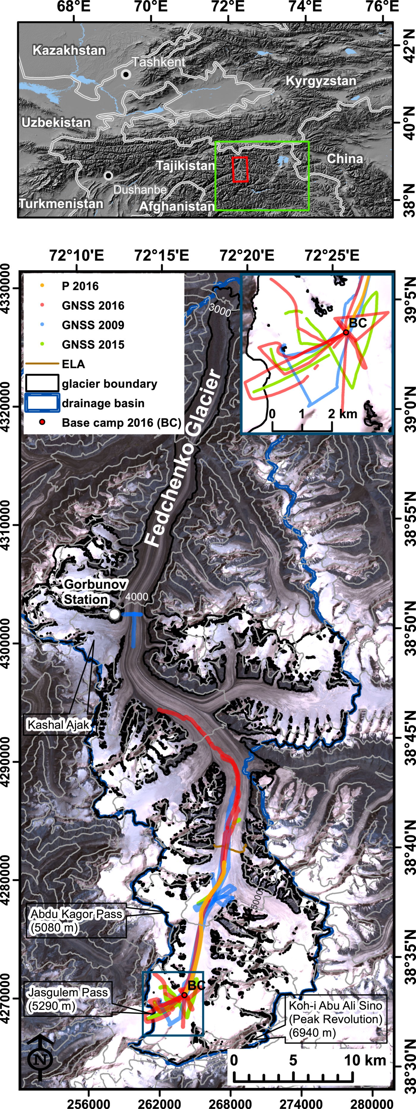
Fig. 1. Location of Fedchenko Glacier (upper panel) and of the GNSS profiles (lower panel) in 2009, 2015 and 2016. The Abdu Kagor pass is just west of the 2009 base camp. The orange profile P from 2016 is used for comparison with GNSS data from 2009. The background image is based on a Landsat 7 scene from 2000, with 500 m contour derived from the SRTM elevation model.
These earlier results demonstrate that the upper regions of this major glacier in the Pamir Mountains experienced rather stable conditions during the first half of the 20th century, followed by a period of volume loss even up to the highest accumulation basins. The contrasting elevation change trends between 2000 and 2009 in the accumulation zone, however, indicate a more complex situation. In this paper, we investigate more recent, ground-based GNSS elevation measurements across the upper part of the glacier, combined with a dense time series of TanDEM-X elevation models. Based on these data we are able to investigate the distributed elevation change pattern along the entire glacier over seasonal to multi-annual timescales.
2. DATA AND METHODS
2.1. Ground-based Global Navigation Satellite Services (GNSS) observations
We used GNSS for ground-based investigations of the glacier geometry, analysing signals from the GPS, GLONASS and Galileo satellites. Positions, including glacier surface elevations, were estimated from GNSS observations during three field campaigns in 2009, 2015 and 2016 (Fig. 1). Besides locations on a rock, which we used as static reference stations, we collected static point observations on the glacier and a total of 194 km of relative GNSS profiles as kinematic tracks. Elevations given in this paper are ellipsoidal heights unless clearly defined differently. Due to different instrumentation and measurement conditions, it was necessary to apply different analysis methods.
In August 2009, the focus was on the region just east of the Abdu Kagor Pass at an elevation of ~4950 m. Two reference stations were established on nearby rock outcrops and the coordinates were computed based on data from the closest International GNSS Service (IGS) reference station Kitab (KIT3). The accuracy of the resulting coordinates was estimated to 1–3 cm for each component in the reference frame IGb08, a realization of the International Terrestrial Reference Frame 2008 (ITRF2008) for the IGS (Dow and others, Reference Dow, Neilan and Rizos2009). The coordinates derived by GNSS and the TanDEM-X elevation models are therefore realized in the same spatial reference system and are thus comparable. The kinematic profiles were collected along the main trunk of the glacier from ~4700 m elevation (just below the ELA) up to a rock outcrop in the upper accumulation basin at ~5400 m elevation. The data from these profiles were processed with respect to one of the two reference stations using the baseline processor WA2 (Wanninger, Reference Wanninger2012), which can analyze GPS, GLONASS and Galileo observations, yielding an expected accuracy better than 5 cm for the height component.
Our 2015 field campaigns concentrated on the upper accumulation basin, where we collected ~32 km of GNSS profiles, including some short profiles further downstream. We processed the data from one GPS-only receiver with the Precise Point Positioning (PPP) method using Terrapos (Gjevestad and others, Reference Gjevestad, Øvstedal and Kjørsvik2007) due to the unexpected failure of the GNSS reference station. PPP is an improved model of the Standard Positioning Service offered by GNSS, including improved estimates of satellite orbits and clocks from, for example, IGS and carrier phase data. The PPP method has a potential for cm accuracy for static applications and sub-decimetre accuracy for kinematic applications, given observation periods of several hours and good satellite coverage. Only a subset of the profiles from 2015 fulfills these requirements.
The majority of the data were collected in 2016, where the GNSS observations started at 4350 m elevation, reaching up to 5400 m and covering a total of 89 km of GNSS tracks. The surface elevation was continuously measured by GNSS during the ascent to the base camp (8–13 August) and on return down-glacier (21–22 August) to our starting point. This time, a GNSS-receiver tracking GPS, GLONASS and the Galileo System was used to estimate the kinematic profiles with PPP. A comparison between the baseline processor WA2 and Terrapos in PPP-mode showed agreement to within ~10 cm in height. The profiles are not along identical tracks in the different years. Therefore, elevation change over time can only be determined either at profile crossing points or where adjacent profiles are very close to each other.
2.2. TanDEM-X elevation models
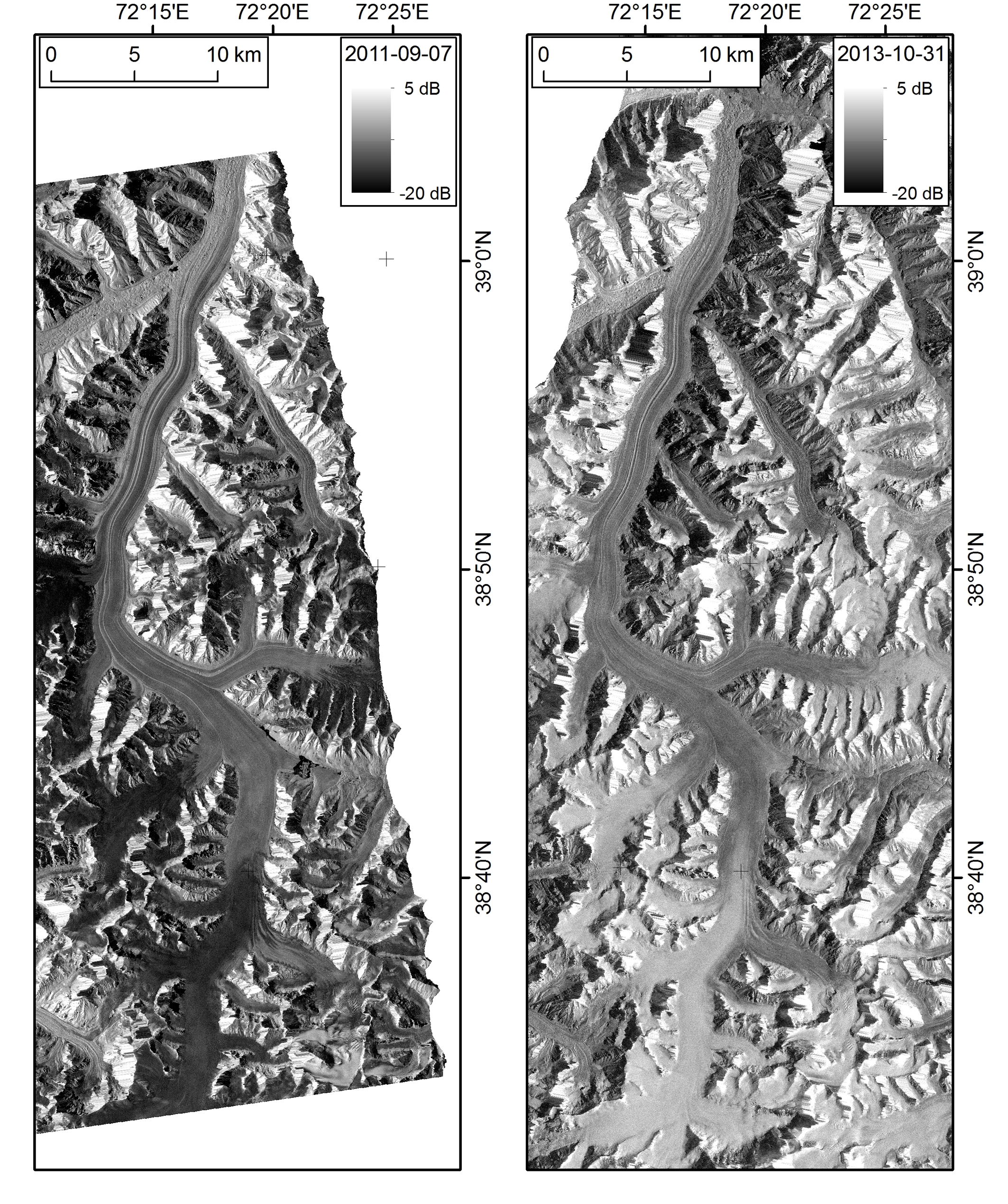
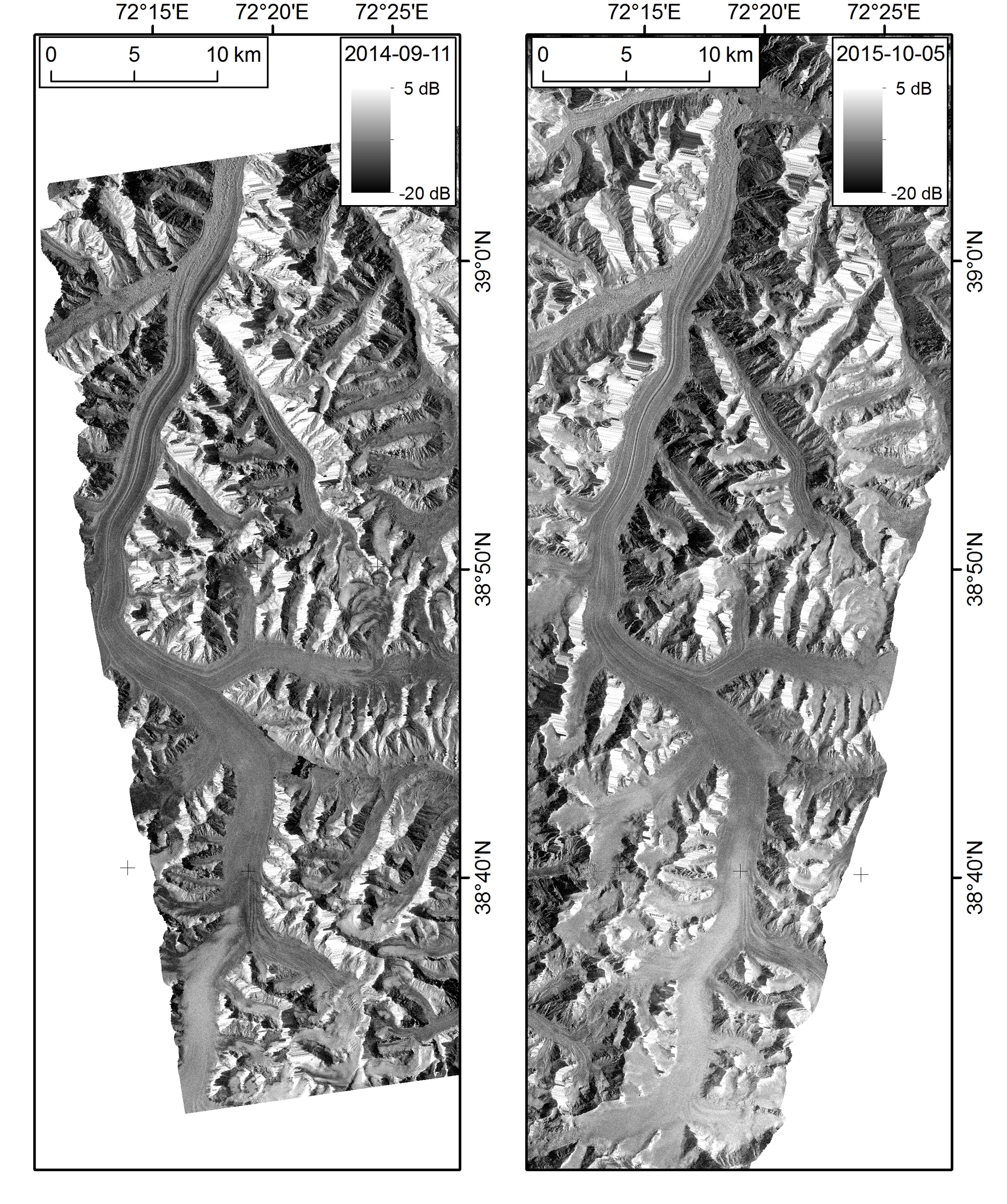
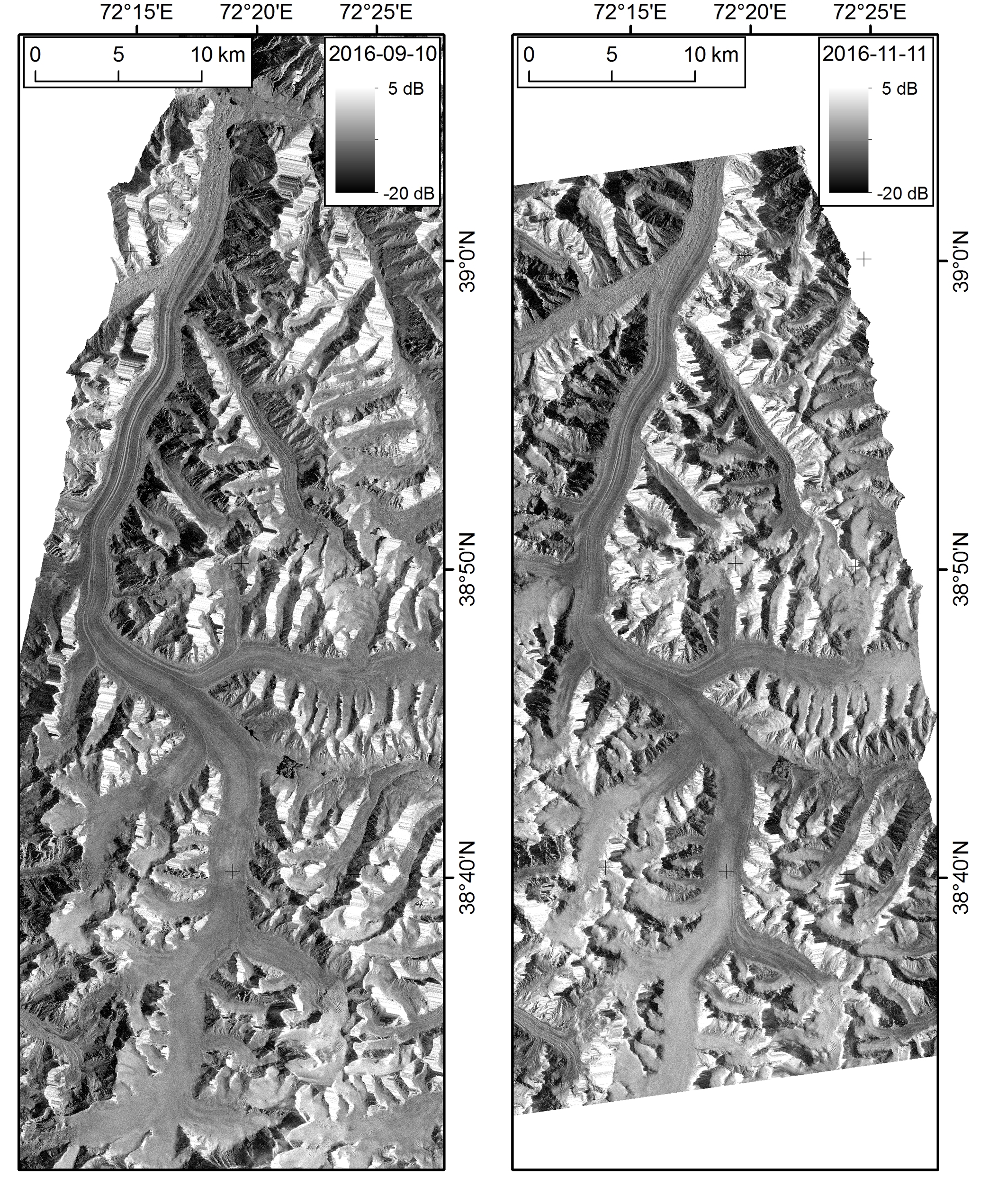
To evaluate glacier-wide elevation changes, we analyzed time series of DEMs derived from synthetic aperture radar (SAR) data of the German TanDEM-X mission. The DEMs were generated from bistatic operational data acquired between 2011 and 2014 for the global TanDEM-X DEM (Krieger and others, Reference Krieger2013) and dedicated science-phase acquisitions scheduled over the glacier mainly in spring and autumn of the years 2011–16 (Table 1). SAR data were processed into pre-calibrated and geocoded DEMs by the Integrated TanDEM Processor (ITP, Rossi and others, Reference Rossi, Rodriguez Gonzalez, Fritz, Yague-Martinez and Eineder2012). Residual phase offsets were determined through comparison with the SRTM DEM and corrected in slant-range geometry within the ITP. Patches of different absolute phase offsets were mosaicked to derive a DEM covering the whole glacier (Wendt and others, Reference Wendt, Mayer, Lambrecht and Floricioiu2017). Together with this DEM, a height error map containing the standard deviations for each pixel based on interferometric coherence and the geometry of the acquisition is provided (Just and Bamler, Reference Just and Bamler1994). To correct for any residual vertical offset between the data takes, all DEMs were registered to a common elevation defined over patches of ice-free flat terrain in the vicinity of the glacier (but outside the map extent of Fig. 1) with a total area of 12.5 km2. The maximum vertical offset of 2.85 m lies within the TanDEM-X DEM specifications defined for the final DEM (Krieger and others, Reference Krieger2013). Due to the sparse occurrence of flat terrain in the vicinity of the glacier, additional adjustment terms such as tilting in range and azimuth were not corrected. Horizontal shifts, which are revealed by an apparent hillshade effect in the elevation differences (Paul and others, Reference Paul2015), were not detected between the individual TanDEM-X DEMs. Table 1 lists the individual data takes including the RMS values over flat terrain. The accuracy of glacier elevations can be worse depending on the particular surface conditions and the associated de-correlation. For the comparison with SRTM data from 2000, a horizontal offset between SRTM and the mean TanDEM-X DEM was corrected by iteratively minimizing elevation differences on bare rock. A residual vertical offset was adjusted over the same flat terrain areas used for the individual TanDEM-X DEMs.
Table 1. TanDEM-X data used in the study, listing orbit direction ascending/descending, perpendicular baseline B⊥, height of ambiguity Ha (defined as the height corresponding to a phase change of 2π) and RMS error over flat ice-free terrain (median slope 4.5°) in comparison with the mean elevation of all DEMs from 2011 to 2014

2.3. Error analysis for TanDEM-X elevations
To estimate errors on the elevation change rates, we divide the error of the elevation differences estimated on bedrock by the time difference between the two DEMs. Therefore, the error decreases for larger time periods.
To evaluate errors σ m of derived mean quantities, the inherent spatial correlation of the data has to be taken into account because neighbouring measurements are not statistically independent (e.g. Rolstad and others, Reference Rolstad, Haug and Denby2009; Willis and others, Reference Willis, Melkonian, Pritchard and Ramage2012). A similar study using SRTM and TanDEM-X to derive elevation change rates for the Patagonian Icefields determined the correlation length to be on the order of 500 m (with a circular correlation area A cor) for glaciated terrain (Abdel Jaber, Reference Abdel Jaber2016). Thus, when calculating the error of a mean elevation change rate, instead of dividing the error of a single measurement σ s by the square root of the number of pixels within the area A under consideration, the dividend is reduced to account for the number of independent measurements (Abdel Jaber, Reference Abdel Jaber2016). The error of the mean quantities therefore given by:
 $${\rm \sigma} _{\rm m} = \displaystyle{{{\rm \sigma} _{\rm s}} \over {\sqrt {9A/2A_{{\rm cor}}}}}. $$
We next integrate the elevation changes over the glacier area to estimate the total volume change. This is then converted into a mass change using a volume-to-mass conversion factor of 850 ± 60 kg m−3, as suggested by Huss (Reference Huss2013) to account for temporal differences in the firn and snowpack.
The uncertainties in volume and mass changes can be evaluated using standard error propagation taking into account the different error components of elevation change rates, glacier area and conversion factor (see e.g. Brun and others, Reference Brun, Berthier, Wagnon, Kääb and Treichler2017). This error estimation considers only stochastic errors. An analysis of systematic elevation errors results in typical magnitudes of ~1 m. This error contribution is included in the error propagation calculation and increases the error estimates of the derived volume and mass change rates by 40% for the period 2011–16 and by 22% for 2000–16.
3. RESULTS
3.1. Analysis of TanDEM-X DEM time series
We derived seasonal, annual and multi-annual DEM differences, based on the available TanDEM-X models in Table 1. The SRTM DEM from 2000 was added to extend the observation period. The varying signal penetration of microwave signals in snow, firn and ice needs to be considered when analysing these differences.
3.1.1. Elevation bias due to microwave penetration for different seasons
To quantify the potential temporal changes in penetration for data of the same wavelength, we derived a time series of elevation changes from TanDEM-X and calculated the backscattering coefficient for one of the accumulation basins of Fedchenko Glacier (Fig. 2). The low-lying Kashal Ajak basin (4300 m), situated near a pass to the Vanj valley receives high snow accumulation in winter and experiences a strong melt and refreezing cycle in spring and summer due to its low elevation. In August 2011 the snow surface was wet and the backscatter was low, indicating that surface (specular) reflection dominates. The determined elevation therefore refers to the snow surface. The same is true for the acquisitions in May 2013 and May 2014. In contrast, all winter observations consistently show elevations, which are between 5.6 and 6.3 m lower, while the September/October observations lie somewhere in between. The respective backscatter (see Figs S1 and S2, supplementary material) indicates that the surface in October 2013 and October 2015 is dry, promoting volume scattering with little signal attenuation and hence relatively high backscatter, while in September 2016 the surface snow layer is likely wet. Part of the observed elevation differences are also due to real changes in surface elevation by accumulation and ablation. However, the rather consistent wet snow summer elevations indicate that this part of the glacier is close to equilibrium between 2011 and 2014. The magnitude of the elevation difference between summer and winter is too large to represent elevation changes due to surface mass balance and dynamic effects, because melt rates of 5–6 m are unrealistic at this altitude and flow velocities are very small. The fact that the observed elevations in winter are lower than in summer documents the penetration difference between wet and dry firn pack conditions, while the cold winter snow on top of the firn layer is transparent as well.
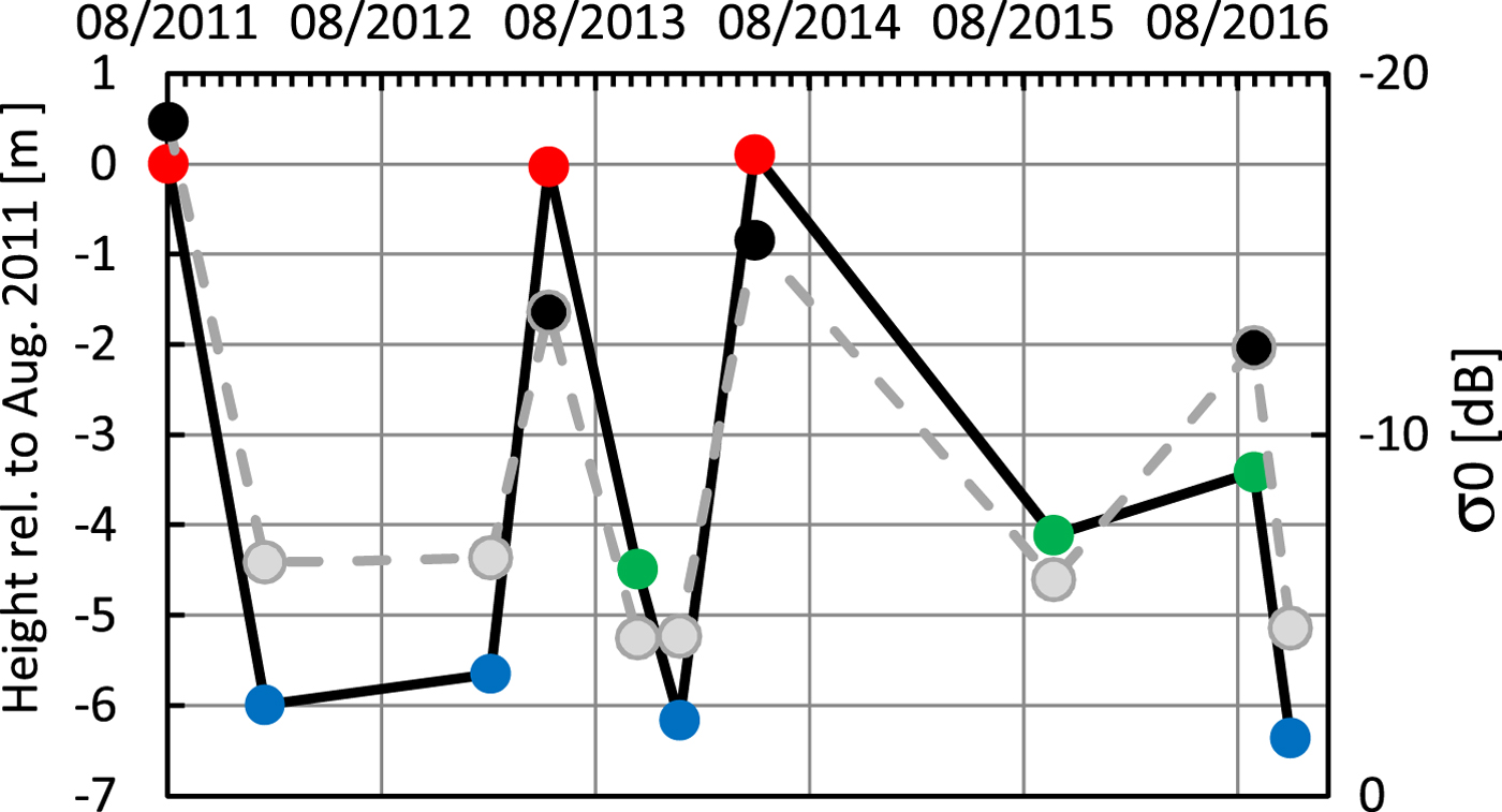
Fig. 2. Elevation changes in the Kashal Ajak (4300 m) accumulation basin (left axis, solid line), relative to August 2011 and the corresponding X-band backscattering coefficient (right axis, dashed line). Late spring and summer observations are marked in red, winter observations in blue and autumn observations in green. Elevations and respective backscatter values are averaged over 4.1 km2 of the accumulation basin.
3.1.2. Seasonal TanDEM-X DEM variation
The comparison of different TanDEM-X elevation models is based on mean elevations calculated across elevation bins (5 m elevation bands) within the main glacier trunk. Using these mean elevations removes small-scale variability, which arises from advection of surface undulations and from InSAR phase noise. A detailed analysis of the period from February 2013 to September 2014, between which there are six available DEMs reveals the pattern of seasonal variations in mean DEM heights along the glacier (Fig. 3). Below the equilibrium line, the differences can be related to real ice surface elevation variations, because cold winter snow is transparent to the X-band signal and we selected late winter scenes without melt conditions. Above the equilibrium line, the signal is a mixture of penetration variations and elevation changes. The autumn/early winter period (October 2013–January 2014, grey line in Fig. 3) shows almost no changes. Below 4800 m elevations, there is a slight height gain, while above this level the change is slightly negative. For late winter/spring (blue lines in Fig. 3) and summer (red/yellow lines in Fig. 3) the changes are considerably larger. A strong elevation increase is observed during the late winter/spring period with maximum values of >4 m between 3400 and 4200 m elevation. The summer periods show an even stronger elevation decrease in the same region, while the height change reverses to positive values in the accumulation area. Elevation changes generally decrease on the debris-covered lower part of the glacier until reaching values close to zero at the glacier tongue.
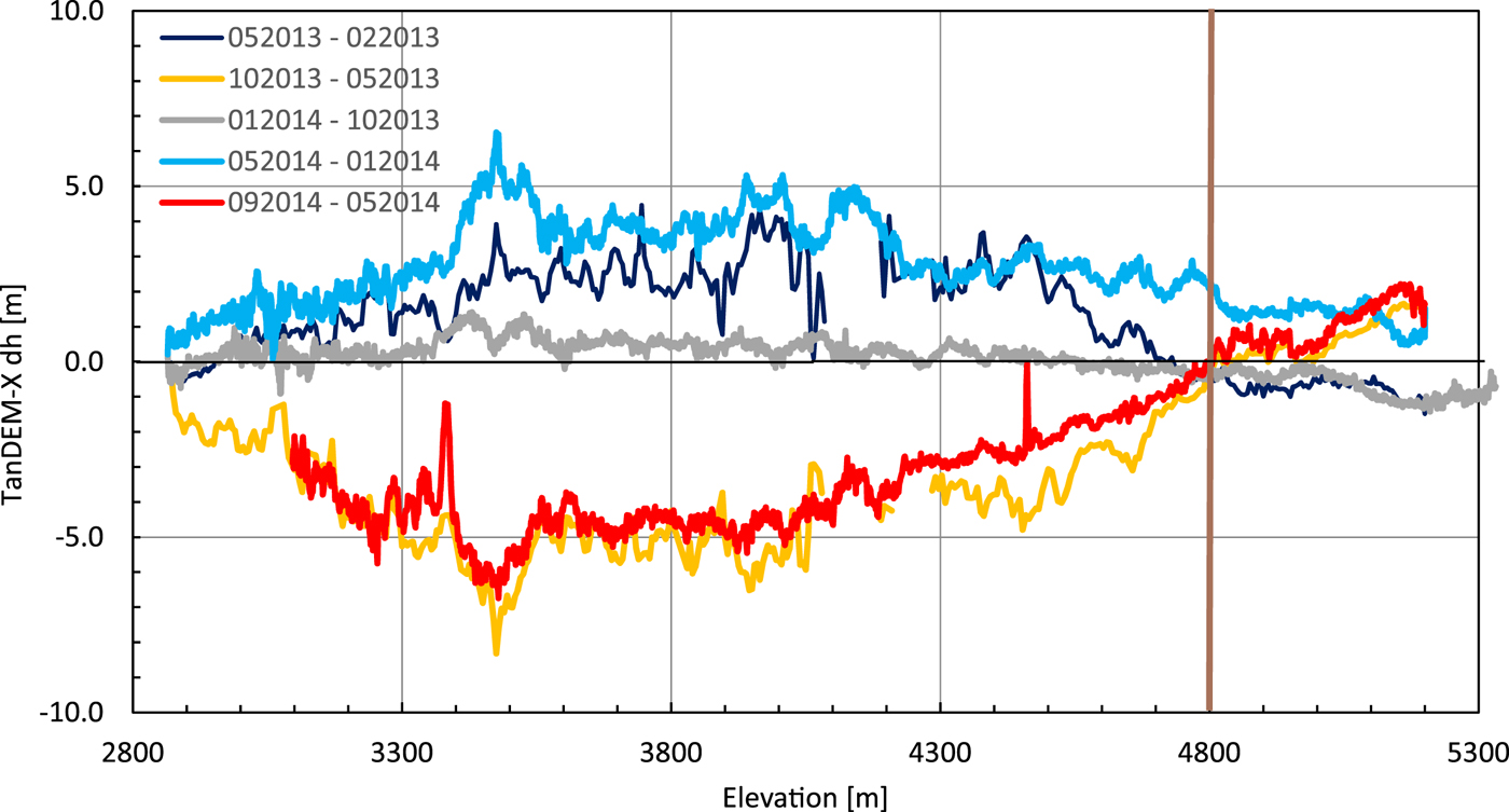
Fig. 3. Comparison of seasonal TanDEM-X DEM differences in the years 2013 and 2014. The grey line shows early winter differences (October – January); blue colours indicate winter/early spring elevation changes, while the red/yellow colours represent summer periods. The brown vertical line shows the ELA.
3.1.3. Annual and multi-annual variations
Elevation changes from InSAR DEMs represent differences in the level of the phase scattering centre, which can be situated at or below the surface, depending on the penetration conditions. Variations in the firn and snow layers can considerably influence the wave penetration, as demonstrated above. There is very little snow cover observed at the end of the melt season in September and October across the ablation zone of the glacier. Hence, this represents the time of minimum firn and snow cover and radar penetration conditions should, therefore, be similar for all image acquisitions at this time of year. The autumn-to-autumn period is also similar to the usual glacier mass-balance year definition and is therefore analyzed here.
Comparing the different periods (Fig. 4) reveals a large interannual variability in elevation changes that have to be interpreted carefully because they lie mainly within the error margins of the DEMs (Tab. 1). In general, a height reduction is observed for most interannual periods. The characteristic annual elevation variation is 1–2 m a−1. We observed no clear elevation dependency of height changes, except for the period 2013/14. The conspicuous peak in most profiles at the confluence of Bivachny Glacier is due to a surge event between 2011 and 2015 (Wendt and others, Reference Wendt, Mayer, Lambrecht and Floricioiu2017). In general, elevation changes are very noisy in the debris-covered lower part of the glacier due to the displacement of pronounced surface undulations.

Fig. 4. Annual and multi-annual elevation change rates between 2011 and 2016 along the main glacier based on TanDEM-X scenes in autumn. The brown vertical line shows the ELA.
Spatial changes in surface conditions and thus radar penetration occur mainly in the accumulation area of Fedchenko Glacier in response, for example, to the up-glacier progression of melting in spring. For the determination of elevation changes, suitable acquisitions have to be carefully selected, aided by the analysis of backscatter (see calibrated backscatter maps in the Supplementary Material S1–S3). In order to evaluate real interannual elevation variations as well as minimizing the influence of different surface conditions, the longest possible time span using comparable data takes should be used to derive an average multi-year elevation change rate. The backscatter between −16 dB and −14 dB (at a 39° incidence angle) in the accumulation area in September 2011 (Fig. S1) indicates wet surface conditions and thus surface scattering.
The comparison of the GNSS-derived elevations in August 2016 and the TanDEM-X elevations from September 2016 (shown below) suggests a negligible penetration of the radar signal into the firn in September 2016. Therefore, the glacier-wide DEMs from 2011 and 2016 should both be free of penetration bias (Fig. 5, right panel). Because both DEMs were acquired in the same month, seasonal dynamic effects can also be neglected. In contrast, surface elevation changes determined from the comparison with SRTM data from February 2000 (Fig. 5, left panel) are influenced by both signal penetration and seasonal dynamic elevation changes. In this case, using a winter TanDEM-X acquisition that also experiences surface penetration into a dry snowpack helps to reduce penetration-related bias when differencing these DEMs, and minimizes the differences due to the seasonal dynamic glacier response. The resulting absolute elevation change rates will represent a lower estimate in the accumulation area because the elevation bias due to penetration is likely to be up to several metres smaller for the TanDEM-X acquisition than for the C- band SRTM DEM. The influence of these effects on the change rate will decrease with time. Therefore, the longest possible period from February 2000 to November 2016 was evaluated here.
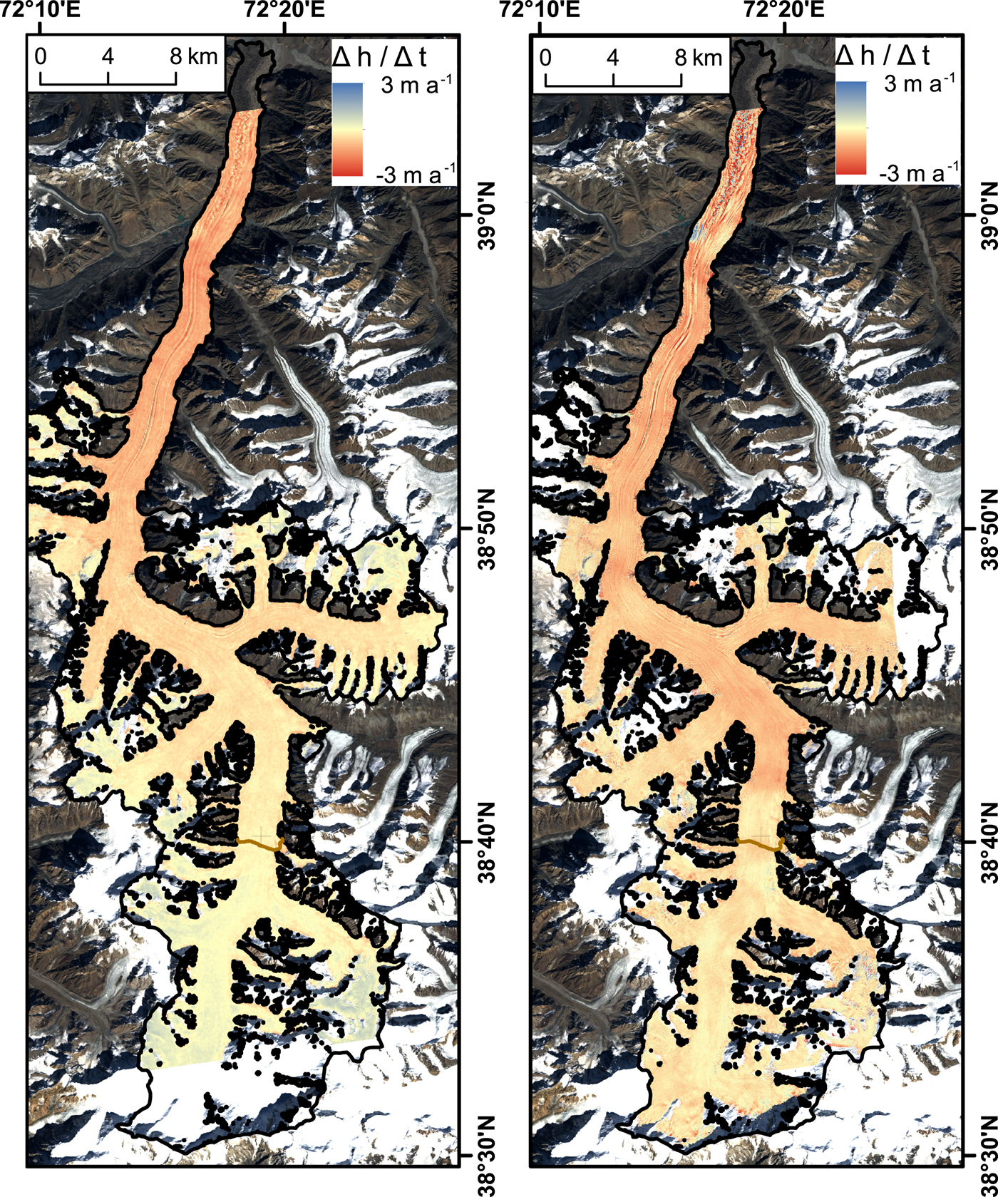
Fig. 5. Elevation change rates for Fedchenko Glacier. The black line indicates the glacier outline, which is covered by most of the TanDEM-X scenes and is therefore used to extrapolate to volume and mass changes. Left: February 2000 (SRTM) to November 2016 (TanDEM-X); right: September 2011 to September 2016 (both TanDEM-X). The brown line indicates the position of the ELA.
The glacier wide mean surface elevations can be directly compared in the ablation zone because microwave penetration into glacier ice or rock debris is a minor issue for X-band data and differences between X- and C-band are small compared with the total elevation variation. In the debris-covered region below 3700 m elevation, the mean thinning rates are 1.20 ± 0.07 m a−1 during the last 16 years, with a maximum of ~1.46 ± 0.26 m a−1 at 3500 m elevation (Fig. 6). This maximum is found just upstream of the confluence with the recently surged Bivachny Glacier (Wendt and others, Reference Wendt, Mayer, Lambrecht and Floricioiu2017). Below this elevation, the thinning is smaller, which might be connected to the increasing supraglacial debris cover, or an additional mass input from the Bivachny Glacier surge. This mass input is, however, limited both in time (between 2014 and 2015) and in space (3300–3400 m elevation). Upstream of 3500 m elevation, the thinning rates decrease almost linearly. At the ELA (4800 m elevation) a thinning of 0.26 ± 0.09 m a−1 is observed in this period (2000–16). The comparison of the elevation change rates for 2000–16 and 2011–16 (Fig. 6) shows a generally similar magnitude of surface lowering. However, the thinning rates since 2011 are somewhat smaller below 3800 m elevation and larger between 4050 and 4700 m elevation, compared with the period since 2000. This leads to a more homogeneous thinning rate of ~1 m a−1 up to ~4650 m. Also, the surface elevation reduction clearly intensified across the entire ablation region, compared with the conditions during the 20th century (1928–2000).
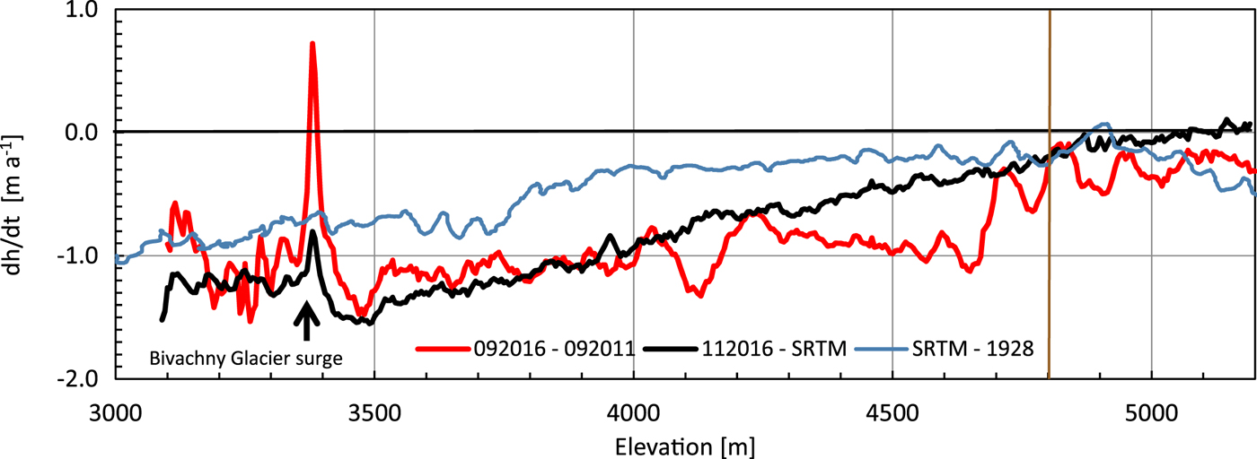
Fig. 6. Longer period elevation change rates along the entire main glacier based on TanDEM-X scenes in autumn and the SRTM elevation model. In addition, the difference of the SRTM DEM and the map elevations from 1928 is provided (Lambrecht and others, Reference Lambrecht, Mayer, Aizen, Floricioiu and Surazakov2014). The brown vertical line shows the ELA.
In the accumulation zone, it is possible to calculate real surface elevation changes for the period 2011–16, because surface scattering can be assumed for both acquisitions, based on the investigation of backscatter maps and the comparison of ground-based GNSS measurements and the TandDEM-X elevations for 2016. The comparison reveals an area-weighted mean elevation decrease of 0.35 ± 0.04 m a−1 above an elevation of 4800 m for Fedchenko Glacier (Fig. 5). In contrast, the mean elevation change rate for the period 2000–16 is close to zero (0.05 ± 0.04 m a−1), with positive rates above ~5000 m. Correcting this result for a gradual penetration increase from 1 m below 4800 m to 4 m above 5300 m results in a mean thinning rate of 0.10 ± 0.10 m a−1. For this calculation, we estimated the X-band versus C-band penetration difference based on a study 50 km east of Fedchenko Glacier (Wendt and others, Reference Wendt, Mayer, Lambrecht and Floricioiu2017). There, C-band penetration depth was up to 4 m deeper than for X-band at an elevation of 5300 m. In addition, we assumed a 50% error in the correction. Elevation increase is thus limited to elevations above 5300 m.
3.2. Elevation changes from GNSS crossing points 2009–16
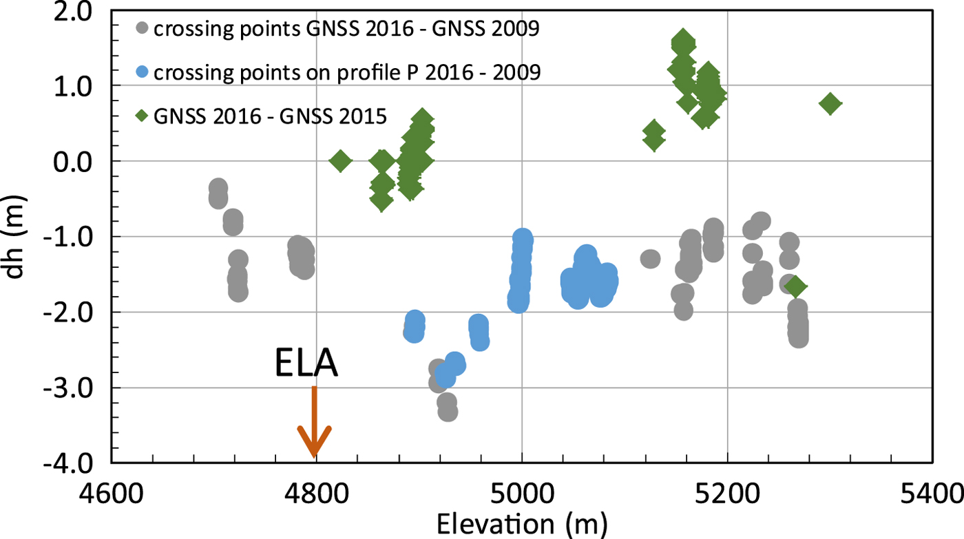
We used crossing points and points of close proximity (<5 m) of the measured GNSS profiles to analyze elevation changes. Surface lowering occurred at all analyzed locations along the main glacier above the ELA (~4800 m altitude) between 2009 and 2016 (Fig. 7). The magnitude of thinning was ~1.5 m above 5000 m elevation, including the crossing points in the main accumulation basin (Fig. 8: blue and grey dots). The plateau close to the Abdu Kagor Pass (~4950 m altitude) shows stronger thinning of >3 m, while down-glacier towards the ELA, it reduces again to values of ~1.3 m and finally ~0.4 m at an elevation of 4730 m during these 7 years. These observations relate to mean elevation change rates of −0.2 m a−1 above 5000 m, −0.4 m a−1 at 4900 m and −0.06 m a−1 just downstream of the ELA. This pattern is also observed for the TanDEM-X elevation differences in the period 2011–16.
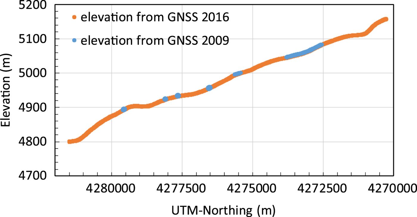
Fig. 7. Surface elevation along the upper glacier section (above the ELA). For the orange profile (measured on 21 August 2016, colour corresponds to Fig. 1) the corresponding elevations from cross profiles and nearby measurements in 2009 are shown in light blue.

In contrast to this 7-year period, the measurements from August 2015 and August 2016 show a mean elevation increase of ~1.3 m above 5150 m elevation in the main accumulation basin and a mean increase of ~0.4 m between 4850 m and 4900 m elevation (Fig. 8: green dots). Because the individual GNSS elevation measurement accuracies are better than a decimetre, these small and locally consistent changes are significant and represent local changes in topography.
3.3. Comparison of TanDEM-X and GNSS elevations in 2016
Elevations derived from GNSS are compared with those derived from TanDEM-X from September and November 2016, the acquisitions closest to the GNSS measurements. Differences calculated for elevation bins of 0.5 m (based on GNSS elevations) show a rather constant offset of ~−2.2 m for the entire elevation range from 4300 to 5400 m between August (GNSS) and September (TanDEM-X), spanning the transition from ablation zone to accumulation zone (Fig. 9). The uniform character indicates a systematic difference between the GNSS measurements and the TanDEM-X model. Furthermore, it suggests that GNSS data in August 2016 and the TanDEM-X DEM from September 2016 essentially sample the same surface without any signal penetration, because penetration is negligible in wet snow and ice surface of the ablation zone below 4800 m (Mätzler, Reference Mätzler1987). Obviously, this is also the case for the snow-covered firn layer of the accumulation zone.
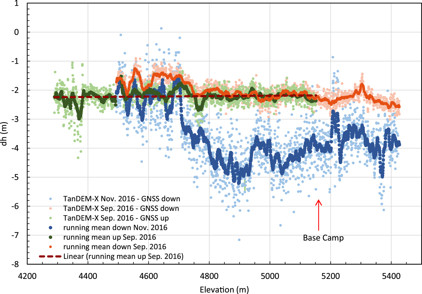
Fig. 9. Elevation differences between GNSS profiles measured when moving up- and down-glacier in August 2016 and TanDEM-X elevation models from September and November 2016. In addition to the differences, running means over 21 differences are displayed, as well as the linear trend for the differences between GNSS-up and TanDEM-X of September 2016.
A systematic elevation offset of ~−3 m between the TanDEM-X elevation model of September 2016 and GNSS observations was found for a ground-control point outside the glacier near Gorbunov station and kinematic measurements on a snow-free medial moraine at 4380 m elevation. This offset (a bias in one or both elevation datasets) explains the major part of the rather constant difference between TanDEM-X elevations of September 2016 and GNSS observations of −2.2 m in Figure 9 (green and orange lines). Comparing the elevation offsets between the TanDEM-X September 2016 DEM and the two sets of August 2016 GNSS measurements when moving up- and down-glacier (separated by an 8–14 daytime span) only shows significant differences between these two datasets below 4750 m elevation. These deviations, which represent elevation differences between mid- and late August in the upper ablation zone, are related to a lower surface due to melt in late August. The mean value of this melt-induced surface lowering is 0.34 m.
The differences between the November 2016 TanDEM-X DEM and the August 2016 GNSS heights are noisier due to a larger height of ambiguity for this TanDEM-X acquisition (Table 1). This results in a higher noise level (Std dev. of 0.72 m) than for the September DEM (Std dev. 0.30 and 0.23 m; light blue points in Fig. 4 compared with the light green and light orange points). Still, the elevation difference to the GNSS data are in the same range of −1.5 to −3 m in the ablation zone. In the accumulation zone, however, the TanDEM-X data from November 2016 are considerably lower (Fig. 9; −3.2 to −5.1 m compared with −2.2 m for altitudes above ~4700 m) which indicates a penetration bias of up to several meters (mean value −1.8 m) in the colder November conditions compared to the warmer conditions in September 2016. These results are comparable with findings in the European Alps, where an elevation bias of 4 m on average is found in the upper glacier accumulation areas (at elevations of ~4000 m) (Dehecq and others, Reference Dehecq, Millan, Berthier, Gourmelen and Trouvé2016).
3.4 Volume and mass changes
For the whole system of Fedchenko Glacier, the derived elevation change rates can be converted to volume change rates using the area-altitude distribution of the glacier. Bivachny Glacier is excluded from this analysis due to its recent surge. Error estimation of the derived volume and mass estimates has been done similarly to Brun and others (Reference Brun, Berthier, Wagnon, Kääb and Treichler2017) as described in Section 2.2. For nonsurveyed portions of the glacier (21% and 13% for 2000–16 and 2011–16, respectively), a doubling of the elevation error has been assumed. The error in glacier area was estimated according to Bolch and others (Reference Bolch, Menounos and Wheate2010) to 5.2%. For the period 2000–16, the uncertainty of the penetration difference between C-band SRTM data and X-band TanDEM-X data has to be accounted for and was conservatively estimated to 50% of the correction itself. The penetration-corrected volume loss amounts to 0.136 ± 0.018 km3 a−1 between 2000 and 2016 on the glacier area covered by both satellite scenes (79% of the total area). Extrapolating this result to the total glacier area with surface slopes <25° (excluding areas with large uncertainties in the TanDEM-X DEMs) results in −0.167 ± 0.032 km3 a−1. With the assumed glacier wide volume to mass conversion factor of 850 ± 60 kg m−3 (Huss, Reference Huss2013) the mass loss rate is 0.142 ± 0.028 Gt a−1, corresponding to a mean mass balance of −0.34 ± 0.07 m w.e. a−1. Similarly, a total volume change rate of −0.246 ± 0.021 km3 a−1 was determined for the period 2011–16, resulting in a mass loss of 0.210 ± 0.025 Gt a−1. The corresponding mass balance is −0.51 ± 0.06 m w.e. a−1 for the period 2011–16.
4. DISCUSSION
The availability of multi-temporal TanDEM-X acquisitions between 2011 and 2016 enables us to analyze seasonal and interannual effects of the interferometrically-determined elevations. Ground-based GNSS observations allow us to adjust elevation offsets of the TanDEM-X DEMs with respect to the ice-free areas and to compare surface elevation changes on the glacier. The comparison of GNSS elevations with TanDEM-X results from the same season also allows a direct estimate of penetration depth variability. Signal penetration of electromagnetic waves into snow and ice has to be considered when interpreting elevation changes based on TanDEM-X differencing, because the elevation of the phase scattering centre results from variable contributions from surface and volume scattering (Mätzler, Reference Mätzler1987). On debris-covered areas and wet glacier ice or snow (with a high dielectric contrast compared with air), surface scattering dominates and signal penetration can be neglected for X-band data. On a wet snow surface, which tends to be smooth at radar wavelengths, the presence of liquid water causes increased absorption and specular reflection, thus directed away from the satellite, resulting in low backscattering and higher phase noise. On dry snow, the radar signal penetrates the surface and is predominantly scattered nonhomogeneously within the snow and firn layers, (e.g. at ice lenses). Fresh, dry winter snow is largely transparent to radar signals due to its low dielectric contrast with air, low density and small grain size.
Our results confirm the earlier observations of a general elevation decrease in the ablation zone. Lambrecht and others (Reference Lambrecht, Mayer, Aizen, Floricioiu and Surazakov2014) reported a long-term mean elevation change rate of almost −0.80 ± 0.09 m a−1 below 3700 m and ~−0.25 ± 0.09 m a−1 from 3700 m up to ~4800 m elevation for the period 1928 until 2000. This thinning reached the glacier regions above 4000 m only after 1958. Surprisingly, the glacier surface seems to have experienced only a minor lowering during the last 88 years in the equilibrium line region between 4700 and 4800 m (Fig. 6). In contrast, the maximum elevation decrease in the period 1928 until 2016 is ~80 m, affecting the region from 2 to ~13 km upstream of the glacier snout (2900–3500 m elevation). The maximum thinning rates of the last 16 years of ~1.50 ± 0.24 m a−1 are almost 1.7 times the long-term 0.90 ± 0.11 m a−1 thinning rates at ~3500 m elevation. This agrees with the general trend of ~1.4–1.5 times higher thinning rates along the entire ablation zone after 2000, compared with the period 1928 until 2000. The region between 4000 and 4700 m elevation experienced an additional intensification of the thinning rates from 2011 until 2016. This results in a more evenly distributed elevation change rate across the ablation area (Fig. 6). Annual and multi-annual elevation change observations (Fig. 4) show a strong variability in time and in space. They very likely reflect variations in mass-balance conditions but also include residual uncertainties. Such short-term elevation differences thus need to be interpreted with care.
The thinning rate of 0.10 ± 0.10 m a−1 found for the accumulation area for the period 2000–16 in this study is somewhat higher than results of an earlier analysis, which indicated close to stable conditions in the accumulation area in the period from 2000 to 2009 (Lambrecht and others, Reference Lambrecht, Mayer, Aizen, Floricioiu and Surazakov2014). However, the significant surface lowering since 2011 of 0.35 ± 0.05 m a−1 indicates a trend towards negative elevation changes in the accumulation area. The analysis of the GNSS measurements extends this period of stronger thinning back to 2009. This is in agreement with observations just below the ELA and indicates a general mass loss across the entire glacier. However, the observed thinning in the accumulation zone could be influenced by increased firn densification due to higher summer temperatures. Year-by-year changes of the glacier surface in the accumulation area can be considerable and depend strongly on the annual accumulation amount. As an example, the glacier surface was generally lower in August 2015 than in August 2016 (Fig. 8), with differences of up to 1.6 m at ~5150 m elevation, but this does not contradict the basic finding of a general long-term lowering in the accumulation area.
The seasonal elevation changes are considerably larger than the annual changes during the analyzed period (Figs. 3 and 4). However, seasonal elevation changes include dynamic effects of submergence and emergence (Cuffey and Paterson, Reference Cuffey and Paterson2010) and the influence of variable signal penetration is difficult to estimate, especially in the accumulation area. In the ablation area, the ice surface elevation will increase during the winter and spring season, because emergence is not compensated by surface melt. In contrast, the surface elevation will lower during the melt season (June–October) because emergence is overcompensated by surface melt. The maximum seasonal elevation difference should occur in the region with the largest melt rates. For clean glaciers, this will be at the glacier snout, while for debris-covered glaciers, the maximum melt rates are likely to be found towards the upper limit of the debris cover. At Fedchenko Glacier, this is at ~3450 m elevation, where the elevation difference is ~12 m between January and September 2014 (Fig. 3). We used surface velocities and surface slope from the TanDEM-X data in combination with simple degree-day melt rates from temperature observations to determine characteristic emergence velocities in the ablation zone, including the influence of an increasing debris cover towards the glacier terminus. We then calculated the temporal elevation change during the ablation and accumulation season based on constant mean emergence velocities. Seasonal elevation changes are smallest close to the ELA and maximum values of ~1–1.5 m are estimated at approximately the upper end of the debris cover (~3400–3500 m elevation). These theoretical elevation changes are very similar to the observed spatial pattern of seasonal elevation change, although the magnitudes are considerably smaller. This variability demonstrates that care is required, when using elevation information from different seasons even in the ablation area, because the seasonal effects might be much larger than the long-term elevation change signal.
A comparison of the resulting mass-balance values to other studies is difficult because only very little information exists for Fedchenko Glacier. Gardelle and others (Reference Gardelle, Berthier, Arnaud and Kääb2013) provide a value for Fedchenko Glacier (including Bivachniy Glacier) of 0.01 ± 0.12 m w.e. a−1 for 2000–11, by comparing Spot 5 data to the SRTM elevation model. However, Kääb and others (Reference Kääb, Treichler, Nuth and Berthier2015) found a higher penetration depth for the SRTM DEM, which might explain the differences between the two studies (Tab. 2). A more recent study by Lin and others (Reference Lin, Li, Cuo, Hooper and Ye2017) also investigated the elevation change of Fedchenko Glacier separately, based on a comparison of SRTM and TanDEM-X elevations, similar to our study. They found a mean elevation change rate of −0.147 ± 0.069 m w.e. a−1 for the period 2000 until 2014, with a strong thinning signal in the ablation area (0.420 ± 0.078 m w.e. a−1) and almost balanced conditions in the accumulation area (−0.028 ± 0.076 m w.e. a−1). The thinning rates in the ablation area are similar to our findings, while our results show considerable thinning also in the accumulation area. This is probably due to the different corrections of the penetration depth. While Lin and others (Reference Lin, Li, Cuo, Hooper and Ye2017) apply a uniform penetration depth of 2 m to the accumulation areas of Western Pamir (and to Fedchenko Glacier), our gradual increase from 1 m at the ELA to 4 m in the upper accumulation area results in a stronger elevation decrease. However, our choice is well based on our observations and thus supports a more negative mass balance. In addition, Lin and others (Reference Lin, Li, Cuo, Hooper and Ye2017) include Bivachniy glacier in their mass-balance estimate, which surged during the end of their observation period. This contributes an additional uncertainty to their analysis.
The mass balance of the Western and Central Pamir Mountains (which are situated in Tajikistan) seems to be negative between 2000 and 2016, even though considerably discrepancies exist between the individual studies (Table 2). While Gardelle and others (Reference Gardelle, Berthier, Arnaud and Kääb2013) found a slightly positive mass balance from 2000 until 2011 (34% of the total glacier area in the Pamir Mountains were surveyed, mainly in the centre), the analysis of altimeter data result in a negative mass balance of different range for 2003 until 2008 (Kääb and others 2015; Gardner and others, Reference Gardner2013). However, they could only analyze small samples of the glacier area, due to the nature of the ICESat footprints and used different methodology and different glacier boundaries in between. A more recent study based on repeat DEMs from ASTER imagery (Brun and others, Reference Brun, Berthier, Wagnon, Kääb and Treichler2017) finds a slightly negative mass balance for the period 2000–16.
Table 2. Summary of the mass balance of the Pamir Mountains based on remote-sensing studies

Compared with the regions of clear glacier area loss in the Western and Central Pamir Mountains (Khromova and others, Reference Khromova, Osipova, Tsvetkov, Dyurgerov and Barry2006), associated with negative mass balances (Table 2) it seems that the Eastern Pamir Mountains represent a transition to more positive mass-balance conditions towards the Kunlun Shan (e.g. Kääb and others, Reference Kääb, Treichler, Nuth and Berthier2015, Lin and others, Reference Lin, Li, Cuo, Hooper and Ye2017).
Interestingly, the mass balance of Fedchenko Glacier is more negative than the respective values for the Western Pamir Mountains in the few existing studies. A comparison of the mass balance of Fedchenko Glacier with the entire Pamir Mountains based on data by Brun and others (pers. comm. January 2018) reveals a clearly more negative mass balance for Fedchenko Glacier (−0.20 m w.e a−1 compared with −0.05 ± 0.08 m w.e. a−1 for the entire region) for the period 2000 until 2016. This is less negative than our mean mass balance of −0.35 ± 0.07 m w.e. a−1 for the same period, but also indicates clearly overall mass loss. A comparison of the absolute values is again difficult, because the methodology is different, especially the calculations for the accumulation area. A reason for the larger mass loss of Fedchenko Glacier compared with the neighbouring regions might be its large extent and the long glacier tongue at comparatively low elevations. A trend towards higher melt rates thus would affect larger areas of the glacier. Our mass-balance determinations of −0.28 ± 0.07 m w.e. a−1 for 2000–11, −0.51 ± 0.06 m w.e. a−1 for 2011–16 and −0.35 ± 0.07 m w.e. a−1 for the entire 2000–16 period also indicate a tendency towards an intensification of the mass loss in recent years.
5. CONCLUSIONS
Fedchenko Glacier shows a substantial volume loss during at least the last nine decades, since the onset of modern observations. The combination of ground-based GNSS observations and SAR remote-sensing data allows a detailed investigation of surface elevation changes between 2000 and 2016. The results extend the record from the earlier topographical maps from the 20th century. The trend of a general surface elevation lowering continues during the investigated period. The mean lowering rates intensified by 1.8 times after 2000 with respect to the multi-decadal rates detected for 1928 until 2000. The new measurements indicate a further intensification of this trend after 2009, especially in the elevation zone from 4000 to 4700 m. While the situation is rather clear for the ablation zone, it is more ambiguous in the accumulation zone. Here, the elevation change rates are considerably smaller, and year-to-year changes are strongly influenced by variations in accumulation rate. This situation, combined with the variable penetration of radar waves in the firn and snowpack, makes it difficult to identify true elevation changes. However, elevation differences with a reasonable accuracy can be determined from TanDEM-X data in the accumulation area, if penetration conditions are similar and the time difference is at least several years. The comparison with ground-based GNSS surface elevation measurements allows the evaluation of the calculated elevation differences and provides estimates for the penetration variability of the X-band radar. The combined analysis of GNSS data and late summer TanDEM-X scenes demonstrates that surface scattering conditions also occur in the accumulation zone. These results emphasize the importance of a careful image selection with similar surface conditions (e.g. taken in the same season) to derive meaningful elevation changes. In this case, DEMs derived from TanDEM-X data are a valuable source for accurate and high-resolution elevation information on glacier surfaces. Our investigations based on GNSS ground observations clearly show thinning in the accumulation zone of up to 0.4 m w.e. a−1. This agrees well with a general trend towards more negative values after 2009–11, when large areas of the accumulation basins are also affected by mass loss.
While inter-seasonal acquisition periods reveal the dynamic glacier response pattern to the mean mass-balance conditions in the ablation zone, such image pairs cannot be used for the analysis of height changes in the accumulation zone. The natural variability is too large, as well as the uncertainties in the detection of the true surface elevation due to radar signal penetration. However, multi-year acquisitions enable the determination of elevation change trends with an accuracy of several cm a−1 and resolve the spatial trend pattern in detail.
The comparison of our results with other recent studies on mass balance in the Pamir Mountains is challenging. Almost all of these studies cover larger regions, which differ in spatial extent and observational time span. Even though the general trends are predominantly negative for the period from 2000 to 2016, the differences are large. Such differences probably also arise from different glacier boundaries and a different handling of glacier areas with no measurements.
Interestingly, Fedchenko Glacier seems to show a more negative mass balance than the larger region (e.g. Gardelle and others, Reference Gardelle, Berthier, Arnaud and Kääb2013; Lin and others, Reference Lin, Li, Cuo, Hooper and Ye2017). This is also confirmed by the comparison of Aster DEMs by Brun and others (pers. comm. January 2018). A potential reason for this situation might be the large size difference and the extensive glacier tongue of Fedchenko Glacier at rather low elevations.
Recent investigations show a strong dependency of the population in the Amu Darya basin on glacier meltwater, especially during drought periods (Immerzeel and Bierkens, Reference Immerzeel and Bierkens2012; Pohl and others, Reference Pohl, Gloaguen, Andermann and Knoche2017). The increasingly negative mass balances of Fedchenko Glacier and especially the strong thinning in the ablation area lead to an intensified water production during the ablation season. This enhanced water supply, combined with the large ice resource of Fedchenko Glacier will serve as an important buffer for water scarcity in the downstream regions.
SUPPLEMENTARY MATERIAL
The supplementary material for this article can be found at https://doi.org/10.1017/jog.2018.52
ACKNOWLEDGEMENTS
The main research for this paper was enabled through funding by the DFG-project LA 1211/3-1. Data was provided through the TanDEM-X projects XTI_GLAC0335, XTI_GLAC7017. We thank Lukas Krieger for providing the backscatter calculations of the TanDEM-X models. We are very grateful to V. Aizen and P. Bohleber for financially supporting the field measurements in 2015. H. Pritchard is greatly acknowledged for improving the style and language of the manuscript. J. Young and an anonymous reviewer provided constructive comments which strongly improved the final paper.


 Open access