


Impact Statement
With the increasing use of complex models for geoscience applications, there is a need for model explainability. It is challenging to apply eXplainable artificial intelligence (XAI) methods to high-dimensional geoscience data because of extensive correlation. We demonstrate how choices in grouping raster elements can substantially influence the relative importance of input features. We also show how differences in XAI output have a relationship with the grouping scheme used. Our work highlights how discrepancies between XAI outputs from different grouping schemes can lead to additional insights about characteristics of the learned features that would not be revealed with a single grouping scheme.
1. Introduction
Geoscience modeling applications are increasingly reliant on artificial intelligence (AI) techniques to develop models that capture complex, nonlinear relationships from geospatial data. Complex deep learning (DL) architectures and high-dimensional raster data inputs are often used to achieve high-performance models. Examples of using DL for geoscience modeling include predicting soil temperature (Yu et al., Reference Yu, Hao and Li2021), typhoon paths (Xu et al., Reference Xu, Xian, Fournier-Viger, Li, Ye and Hu2022), tropical cyclones (Lagerquist, Reference Lagerquist2020), sea-surface temperature (SST) (Fei et al., Reference Fei, Huang, Wang, Zhu, Chen, Wang and Zhang2022), and classification using multi-spectral (Helber et al., Reference Helber, Bischke, Dengel and Borth2019) and synthetic aperture radar (Zakhvatkina et al., Reference Zakhvatkina, Smirnov and Bychkova2019). Many studies demonstrate that the complexity enables the model to achieve the desired predictive skill, but the complexity also makes it very difficult to understand the model’s decision-making process. There are many examples where models appeared to achieve high performance based on evaluation against an independent testing dataset, but actually learned to exploit spurious relationships that are not useful for real-world use (Lapuschkin et al., Reference Lapuschkin, Wäldchen, Binder, Montavon, Samek and Müller2019). Or, a model may have learned to use patterns existing in nature that are unknown to human experts (Quinn et al., Reference Quinn, Gupta, Venkatesh and Le2021). These are potential opportunities to learn novel scientific insights by exposing a model’s learned strategies. Model debugging and scientific inquiry are two major motivations behind the rapidly developing field of eXplainable AI (XAI). XAI approaches are usually categorized as either interpretable models or post-hoc explanation methods (Murdoch et al., Reference Murdoch, Singh, Kumbier, Abbasi-Asl and Yu2019). Interpretable models are machine-learning (ML) methods for constructing models with inherent explainability. While these models are easier to understand, they are usually much simpler than the complex architectures required for complex geoscience applications. Instead, we focus here on post-hoc explanation methods that are applied to arbitrary models to investigate what they have learned.
XAI techniques tend to struggle with correlated data, and can produce very misleading explanations (Au et al., Reference Au, Herbinger, Stachl, Bischl and Casalicchio2022). This limits the potential for XAI to explain geoscience models since many rely on gridded geospatial input data that contain extensive correlation (Legendre, Reference Legendre1993). In addition to long-range dependencies (e.g., teleconnections (Niranjan Kumar and Ouarda, Reference Niranjan Kumar and Ouarda2014)), high autocorrelation among grid cells is very often present because of spatial and temporal relationships among them. As the dimensionality of the geospatial input data increases, it becomes more challenging to achieve reliable and meaningful explanations from XAI methods. The approach taken by many post-hoc methods is not well-suited to data with high autocorrelation. These methods explain the model by modifying the input data and evaluating the model to measure the change in either performance or output (Lundberg and Lee, Reference Lundberg, Lee, Guyon, Luxburg, Bengio, Wallach, Fergus, Vishwanathan and Garnett2017). The problem is that these methods evaluate the influence of single grid cells, but the model learns spatial patterns within the gridded input. A single cell often has minimal information for the model. For example, a model that detects clouds in an image should not be concerned with a single grey pixel. Instead, groups of grey pixels with certain textural patterns are recognized as cloud features. By analyzing models at the cellular level, grid cells that are part of learned patterns may not be detected as being influential. Because of this problem, it is very easy to produce misleading explanations with XAI.
A proposed solution is to group correlated features before applying XAI (Au et al., Reference Au, Herbinger, Stachl, Bischl and Casalicchio2022). Then, post-hoc XAI methods perturb group members together to explain that feature. While individual grid cells may have minimal impact on the model, removing the set of correlated features could trigger considerable change. This has become common for tabular data where the correlation matrix is used to group correlated features. This makes sense for relationships that hold across a dataset, such as between variables height and weight. This does not apply to the image patterns that are present in raster data. There is very little research on strategies for grouping grid cells to improve the quality of explanations produced by XAI methods, especially for rasters other than RGB or grayscale images. Groups may be formed by clustering in a data-driven fashion or by partitioning the raster according to a geometric grouping scheme. Either way, there is little guidance on how the choice of groups influences the explanations.
In this research, we analyze how the geometric partitioning scheme influences XAI. We show that explanations from different grouping schemes can greatly disagree. Based on the grouping scheme, users could have opposite interpretations of which features are influential. Many studies have demonstrated that XAI methods may disagree (McGovern et al., Reference McGovern, Lagerquist, Gagne, Jergensen, Elmore, Homeyer and Smith2019), but there is little research concerning the disagreement that arises based on feature grouping, especially for high-dimensional geospatial data. One conclusion is to avoid XAI since it is unclear which explanation is correct. Here, we aim to show that the disagreement may reveal insights about the nature of the learned features. Each explanation should be considered the answer to a specific question rather than a complete model summary. We apply a hierarchy of partitioning schemes and demonstrate interpreting the model based on the set of explanations to extract information about the scale of the learned features. FogNet, a DL model for predicting coastal fog in the South Texas Coastal Bend (Kamangir et al., Reference Kamangir, Collins, Tissot, King, Dinh, Durham and Rizzo2021), is used to analyze the impact of partitioning the raster elements into features for XAI. It was chosen because of its complex architecture and high-dimensional raster input.
To summarize, there is a desire to use XAI to investigate complex geoscience models, but the strong correlations in the geospatial raster data make it easy to be misled by XAI outputs. While some researchers are using XAI for geoscience models (Cilli et al., Reference Cilli, Elia, D’Este, Giannico, Amoroso, Lombardi, Pantaleo, Monaco, Sanesi, Tangaro, Bellotti and Lafortezza2022; Sachit et al., Reference Sachit, Shafri, Abdullah, Rafie and Gibril2022), there is little investigation of explanation quality. We have two major goals: (1) to expose that the correlations in geospatial data can cause misleading explanations and (2) to offer guidance toward better model understanding by carefully applying multiple XAI methods at a hierarchy of feature grouping schemes. It is difficult to verify XAI methods because the true explanation is, in general, not known. However, we analyze the consistency among methods and rely on domain expertise to relate the discrepancies between XAI outputs to the underlying physics of the features. Based on our analysis, we feel confident that, while no XAI method is perfect, our XAI strategy is revealing overall patterns related to how features at different scales influence model decisions.
Our work provides the following contributions:
-
1. Demonstration that XAI methods are highly sensitive to the feature grouping scheme.
-
2. Presentation of strategies for using multiple grouping schemes for deeper model insights.
-
3. Presentation of strategies for aggregating local explanations into global explanations.
-
4. Development of modified PartitionShap (Lundberg and Lee, Reference Lundberg, Lee, Guyon, Luxburg, Bengio, Wallach, Fergus, Vishwanathan and Garnett2017) for multichannel rasters explanations.
-
5. Demonstration of how our XAI strategies can help a domain expert better interpret a complex model.
The paper is organized as follows. Section 1 introduces the problem and our contributions, followed by a review of related research. Section 2 describes FogNet and its geospatial input raster. The section then describes the XAI methods applied to that model and the various grouping schemes used. Section 3 presents the results of our experiments and Section 4 provides our interpretation of the explanations. We demonstrate that an understanding of the methods in Section 2, along with domain knowledge, helps us better interpret XAI outputs even when there are substantial discrepancies among them. Finally, Section 5 summarizes our findings and offers guidance to practitioners using XAI for geoscience models.
1.1. Related works
In the following three examples, models use DL architectures with gridded spatiotemporal predictors, and comparisons with simpler alternative models highlight performance gains using the more complex architecture. Yu et al. (Reference Yu, Hao and Li2021) used spatiotemporal rasters to predict soil temperature. A DL architecture was developed with three-dimensional (3D) convolution to learn spatial-temporal features and significant performance gains were achieved over simpler 2D convolution. Xu et al. (Reference Xu, Xian, Fournier-Viger, Li, Ye and Hu2022) developed a DL model for typhoon path prediction. Comparing several ML techniques and DL configurations, the best architecture was a fusion of DL with 3D convolution and a Generalized Linear Model. Fei et al. (Reference Fei, Huang, Wang, Zhu, Chen, Wang and Zhang2022) developed a hybrid model for bias-correcting SST from raster numerical weather model output. A convolutional long short-term memory (LSTM) model was used to learn spatial-temporal patterns. These performance gains achieved using complex models motivate our study of post-hoc XAI for geoscience modeling rather than interpretable models.
Researchers have begun to adopt XAI methods to explain these complex atmospheric models. McGovern et al. (Reference McGovern, Lagerquist, Gagne, Jergensen, Elmore, Homeyer and Smith2019) reviewed XAI for meteorological ML which regularly uses high-dimensional spatial-temporal rasters. Several techniques were used to explain a tornado prediction CNN that uses a multi-channel raster of atmospheric variables. The study highlights that discrepancies between XAI methods explanations are common, and they caution against bias confirmation: to not assume that the explanation that matches expectations is the most accurate. Instead, the recommended strategy is to apply multiple XAI methods; consistencies provide evidence of the true explanation. Lagerquist (Reference Lagerquist2020) developed a CNN to predict the probability of next-hour tornado occurrence based on storm-centered radar imagery and proximity soundings. To explain the model, the authors applied several XAI techniques. The authors performed additional XAI verification using sanity checks proposed by Adebayo et al. (Reference Adebayo, Gilmer, Muelly, Goodfellow, Hardt and Kim2018) who observed that explanations are sometimes overly influenced by input discontinuities. Some XAI methods may highlight raster edges rather than explain influential features. Lagerquist (Reference Lagerquist2020) applied these sanity checks, which suggest that the explanations are in fact based on model behavior. Hilburn et al. (Reference Hilburn, Ebert-Uphoff and Miller2021) used Geostationary Operational Environmental Satellite (GOES) imagery to train a U-Net architecture to estimate the spatial distribution of composite reflectivity. Layer-wise Relevance Propagation (LRP) identifies influential raster elements using a backward pass through the neural network. In the GLM channel of the input raster, LRP results suggest that the network focuses on lightning regions. The authors then created modified inputs, removing the lighting in the GLM channel to observe model output. The results indicated that the lightning did in fact contribute significantly. Here, an existing XAI technique was used, but with additional steps taken to increase confidence. A fundamental XAI challenge is the lack of a ground truth to determine if the explanation is correct. The above authors show how additional steps can be taken to increase confidence in explanations: explanation consistency (McGovern et al., Reference McGovern, Lagerquist, Gagne, Jergensen, Elmore, Homeyer and Smith2019), sanity checks (Lagerquist, Reference Lagerquist2020), and synthetic inputs (Hilburn et al., Reference Hilburn, Ebert-Uphoff and Miller2021).
Correlations among input features can cause XAI techniques to provide misleading explanations. The rasters used in geoscience modeling often have a substantial spatial correlation among grid cells. A potential solution is to group correlated features. Au et al. (Reference Au, Herbinger, Stachl, Bischl and Casalicchio2022) describe the XAI challenges caused by correlated input features, and describe three variants of XAI algorithms for explaining groups of features: permutation feature importance (PFI), refitting (retraining the model with the group removed), and LossSHAP. Initial efforts have been made in grouping pixels of RGB/grayscale image pixels into feature groups for XAI. Ribeiro et al. (Reference Ribeiro, Singh and Guestrin2016) includes superpixel clustering before explaining image-based models in the LIME software package. Observing that the size and shape of superpixels influenced XAI results, Hajiyan (Reference Hajiyan2022) proposed recursively dividing larger superpixels into increasingly smaller ones. LIME was applied to each set of clusters, from largest to smallest. Based on the size of the learned pattern, the influence of a pixel may be detected only at a certain level of granularity. The LIME outputs from each level of the hierarchy were summed so that a single explanation highlights pixels whose influence was detected at any level. Here, we do not combine the XAI results from different grouping schemes because our goal is to show that each grouping scheme’s result should be interpreted differently. Information about the scale of the learned patterns is lost when combining them, especially for high-dimensional, multi-channel geospatial data.
2. Methods
2.1. FogNet
FogNet (Kamangir et al., Reference Kamangir, Collins, Tissot, King, Dinh, Durham and Rizzo2021) is a DL architecture for predicting coastal fog that outperforms the operational high-resolution ensemble forecast (HREF) across several performance metrics (Kamangir et al., Reference Kamangir, Collins, Tissot, King, Dinh, Durham and Rizzo2021). Here, the model was trained for 24-h lead time predictions for visibility <6400 m. Features were derived from the North American Mesoscale Forecast System (NAM). An additional feature is observed SST from the NASA Multiscale Ultra-high Resolution (MUR) satellite dataset. The target visibility data is observations at Mustang Beach Airport in Port Aransas, Texas (KRAS). The gridded inputs are concatenated to create an input raster of shape (32, 32, 384). The target is a binary class representing whether or not there is visibility at the specific threshold. Variables were selected to capture 3D spatial and temporal relationships related to fog. The FogNet architecture was designed to capture relationships across both the spatial grids and the spatial-temporal channels using dilated 3D convolution (Kamangir et al., Reference Kamangir, Collins, Tissot, King, Dinh, Durham and Rizzo2021).
The FogNet input (Figure 1) is divided into 5 groups of related physical characteristics. These features are described in the FogNet paper (Kamangir et al., Reference Kamangir, Collins, Tissot, King, Dinh, Durham and Rizzo2021). G1 contains a 3D profile of wind data. G2 features include turbulence kinetic energy (TKE) and specific humidity (Q). G3 approximates the thermodynamic profile by including relative humidity (RH) and temperatures (TMP). G4 features account for surface moisture (q) and air saturation (dew point depression) as well as microphysical features such as NAM surface visibility and temperature at the lifted condensation level (TLCL). G5 includes both the SST analysis product from the MUR as well as derived values: the difference between SST and temperature (TMP-SST) and the difference between dew point temperature and SST (DPT-SST).
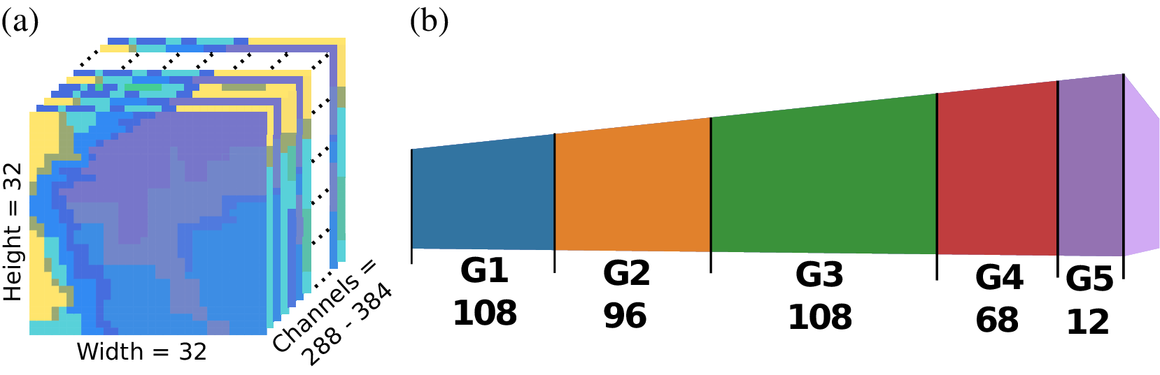
Figure 1. The FogNet input (a) has 384 channels, forming ifve groups of physically-related variables (b).
Although these groups contain features that relate to a particular fog-generating or dissipating mechanism or possess a statistical correlation to fog occurrence, there exist correlations across the groups. For example, Groups 1, 2, and 3 are correlated; a temperature inversion (temperature increase with height) in the lower levels (G3), which typically occurs during fog events, will result in an atmospheric condition known as positive static stability (Wallace and Hobbs, Reference Wallace and Hobbs1977) which will suppress vertical mixing of air which in turn affects surface wind velocity (G1). Furthermore, a thermal inversion can suppress turbulence (G2) (Stull, Reference Stull1988). Groups 3 and 5 are related since G3 contains surface RH, which is inversely proportional to the G5 feature dew point depression. Since wind has a turbulence component, there exists a relationship between G1 wind and G2 TKE. In addition, G1 and G4 are related since surface wind divergence (convergence) results in downward (upward) VVEL immediately aloft.
2.2. Explainable artificial intelligence
FogNet is used to compare XAI results when grouping raster elements with 3 different feature grouping schemes. To explain the feature importance of these groups, we use the three group-based XAI techniques discussed by Au et al. (Reference Au, Herbinger, Stachl, Bischl and Casalicchio2022). In addition, we use a feature effect method called PartitionSHAP (Hamilton et al., Reference Hamilton, Lundberg, Zhang, Fu and Freeman2021) using our version called Channel-wise PartitionSHAP that we extended to explain multi-channel raster inputs. Figure 2 shows several geometric partition schemes, but this is not exhaustive since groups can be arbitrarily complex in shape.
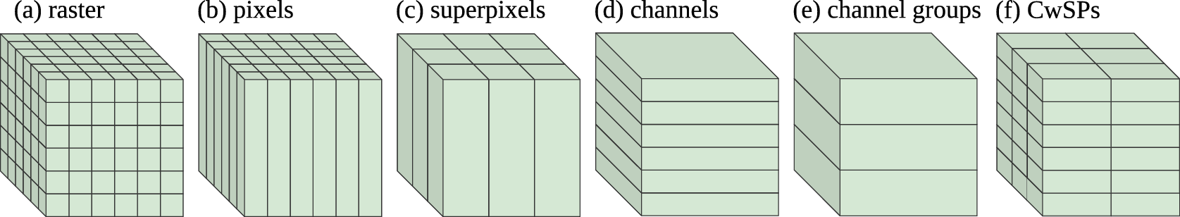
Figure 2. Various geometric schemes to group 3D rasters. The most granular is the (a) raster itself where no grouping is applied. Each spatial element can be grouped into a (b) pixel that contains all channels at that (row, column) location. Adjacent pixels may be combined into coarser (c) superpixels. Similarly, adjacent (d) channels may be aggregated into (e) channel groups. Within each channel, the elements may be aggregated into (f) channel-wise superpixels (CwSPs).
Here, FogNet features are grouped using three schemes. The least granular is the five physics-based channel groups (Figure 1b). Our ablation study (Kamangir et al., Reference Kamangir, Krell, Collins, King and Tissot2022) confirmed that each contributes to FogNet’s high performance. So we expect that each group should be assigned significant importance. Next, each of the 384 channels is also used as a feature (Figure 2d). Ideally, this reveals more insight into the model: which variables, at what altitudes, and time steps are used. An issue is that there is already a risk of highly correlated channels diluting the detection of each channel’s true influence. To assess sensitivity, we sum channel-wise XAI values to see if the summations achieve the same group ranking as the channel groups XAI. To achieve spatial-temporal explanations, the lowest level of granularity is channel-wise superpixels (Figure 2f). We will assess sensitivity by aggregating superpixels in each channel for comparison with channel-wise XAI and further aggregate into groups to compare to group-based XAI.
We must consider the explanation’s meaning: what, exactly, the method does to calculate these values to better understand what they reveal about the model. Consider applying PFI to a single grid cell. After permuting multiple times and taking the average of the change in model performance, we may find a near-zero importance score. As discussed, single-element changes are likely to have little influence on the model in isolation. That does not mean that there cannot be single elements that do have high importance scores. When the importance score of a grid cell is low, it tells us that the single pixel in isolation is not important. When the score is high, that grid cell greatly impacts the model by itself. If PFI at the grid cell level outputs very low importance scores, a reasonable interpretation is that the model does not rely on such fine-grained information to make decisions. This is desirable when the target is correlated with patterns rather than the value at a single location. In the case of fog, forecasters rely on the air temperature profile rather than temperature at a particular level. 2D and 3D CNNs are chosen when we expect that patterns are crucial for forecasting skill.
Next, suppose that PFI revealed several important superpixels, but did not reveal important pixels. This suggests that the CNN is in fact learning to recognize patterns within 2D gridded data. This is an example where the discrepancy between XAI applied at two grouping schemes reveals insight into the model that could not be determined using either grouping scheme alone. In this research, we propose that XAI applied to multiple grouping schemes can offer insight into model behavior. This is in contrast to a conventional take that differences between XAI methods mean that there is a problem with one or more of the methods. The key to interpreting a set of explanations is to understand that each asks a different question of the model.
2.3. Feature effect methods
Feature effect methods quantify each feature’s influence on a specific output. Unlike importance methods, feature effect reveals features being used by the model regardless of their impact on performance. The positive and negative impact on performance may cancel out such that a very influential feature is not detected by a feature importance method. These are called local methods because the explanation is for a specific output; it may reveal non-physical strategies that rarely occur, useful for imbalanced datasets.
It can be challenging to obtain insights from a large set of high-dimensional local explanations. Each is a raster of values with the same dimensions as the input. Instead of a single global explanation for the model, local explanations can be aggregated by category. Lagerquist (Reference Lagerquist2020) combined XAI results by extreme cases: best hits, worst misses, etc. In our case, the FogNet input rasters have consistent grid cell geography. That is, each has identical geographic extent and resolution such that (row, col) coordinates always align spatially across samples. We take advantage of this to aggregate explanations by summing values at each coordinate across a set of samples as shown in Section 2.3. This converts the set of local explanations into a much smaller set of figures that can be analyzed more easily, at the loss of case-by-case granularity.
Local explanations of rasters are often visualized with an attribution heat map: a 2D image where the colors correspond to the relative influence of that grid cell’s attribution toward the model output. Commonly, red values indicate a positive contribution while blue indicates a negative. A single heatmap is typically used to explain grayscale and RGB samples but is not informative for arbitrary multi-channel rasters. Figure 7 shows an example where each heatmap corresponds to a single raster channel.
2.3.1. SHapley Additive ExPlanations
Game-theoretic Shapley values are the fairly distributed credit to players in a cooperative game (Lundberg and Lee, Reference Lundberg, Lee, Guyon, Luxburg, Bengio, Wallach, Fergus, Vishwanathan and Garnett2017). Each player should be paid by how much they contributed to the outcome. In the XAI setting, the features can be considered players in a game to generate the model output. Thus, a feature that influenced the model to a greater extent is a player that should receive more payout for their contribution. Shapley values are a feature’s average marginal contribution to the output. Calculating Shapley values directly has combinatorial complexity with the number of features. Since it is infeasible for high-dimensional data, Lundberg and Lee (Reference Lundberg, Lee, Guyon, Luxburg, Bengio, Wallach, Fergus, Vishwanathan and Garnett2017) developed a sampling-based approximation called SHapley Additive exPlanations (SHAP). Molnar et al. (Reference Molnar, König, Herbinger, Freiesleben, Dandl, Scholbeck, Casalicchio, Grosse-Wentrup and Bischl2020) gives a detailed explanation of SHAP and its advantages and disadvantages.
A single contribution is the difference between the model output with and without a feature $ x $
. The challenge is that models usually expect a fixed input and do not support leaving out a feature. Feature removal has to be simulated somehow, and a variety of methods have been proposed. In canonical SHAP, the value of the removed feature
$ x $
. The challenge is that models usually expect a fixed input and do not support leaving out a feature. Feature removal has to be simulated somehow, and a variety of methods have been proposed. In canonical SHAP, the value of the removed feature $ x $
is replaced with the value from
$ x $
is replaced with the value from $ x $
in other dataset examples. By replacing
$ x $
in other dataset examples. By replacing $ x $
with many such values and averaging the result, SHAP evaluates the average difference in output between the true value of
$ x $
with many such values and averaging the result, SHAP evaluates the average difference in output between the true value of $ x $
and output without that value.
$ x $
and output without that value.
The key to Shapley values is that many additional output comparisons are performed to account for feature dependencies and interactions. In the context of a cooperative game, consider a team that has 2 high-performing players $ x $
and
$ x $
and $ y $
. The remaining players on the team have no skill. With
$ y $
. The remaining players on the team have no skill. With $ x $
and
$ x $
and $ y $
playing, the team wins despite no help from the others. The goal is to fairly assign payout to the players based on their contribution to the game’s outcome. Suppose
$ y $
playing, the team wins despite no help from the others. The goal is to fairly assign payout to the players based on their contribution to the game’s outcome. Suppose $ x $
is removed from play and
$ x $
is removed from play and $ y $
is still able to win the game. Comparing the two games, one could conclude that
$ y $
is still able to win the game. Comparing the two games, one could conclude that $ x $
did not contribute to the win. Instead, if
$ x $
did not contribute to the win. Instead, if $ y $
were removed and
$ y $
were removed and $ x $
wins the game then it appears that
$ x $
wins the game then it appears that $ y $
does not contribute, but removing both
$ y $
does not contribute, but removing both $ x $
and
$ x $
and $ y $
causes the team to lose the game. Thus, the change in outcome from player
$ y $
causes the team to lose the game. Thus, the change in outcome from player $ x $
depends on player
$ x $
depends on player $ y $
.
$ y $
.
The combinatorial complexity is because it takes the above dependency issue into account. To evaluate the contribution of $ x $
, it does more than just compare model outputs with and without
$ x $
, it does more than just compare model outputs with and without $ x $
present. It repeats the comparison but considers all possible combinations of other players being present or absent from the game. A feature’s Shapley value is a weighted average of the contribution over all the possible combinations of players. SHAP approximates the Shapley values over a set of samples for performance, but still potentially requires a very large number of evaluations to converge to a close approximation.
$ x $
present. It repeats the comparison but considers all possible combinations of other players being present or absent from the game. A feature’s Shapley value is a weighted average of the contribution over all the possible combinations of players. SHAP approximates the Shapley values over a set of samples for performance, but still potentially requires a very large number of evaluations to converge to a close approximation.
2.3.2. PartitionSHAP
It is impractical to use SHAP for FogNet’s channels or channel-wise superpixels because of the large number of features. PartitionSHAP (Lundberg and Lee, Reference Lundberg, Lee, Guyon, Luxburg, Bengio, Wallach, Fergus, Vishwanathan and Garnett2017) uses hierarchical grouping to approximate Shapley values for superpixels with a significantly reduced number of calculations. The complexity of PartitionSHAP is quadratic with the number of raster elements instead of SHAP’s exponential complexity. Given a partition tree that defines a hierarchy of feature groups, PartitionSHAP recursively traverses the tree to calculate Owen values. These are equivalent to Shapley values for a linear model but otherwise have their own properties useful for dealing with correlated features. Unlike Shapley values, the recursive Owen values are able to correctly assign credit to groups even if the correlated features are broken while perturbing those features, but this is only true if the partition tree groups correlated features.
For tabular data, PartitionSHAP uses a clustering algorithm to define the partition tree. For rasters, PartitionSHAP partitions by recursively dividing the data into 2 equal-size superpixels. Figure 3a shows the first 4 levels of a partition tree constructed for a single-channel raster. The root is the largest group, the entire image. Each node’s children represent splitting it into 2 superpixels. PartitionSHAP’s image partitioning algorithm is illustrated in Figure 4.
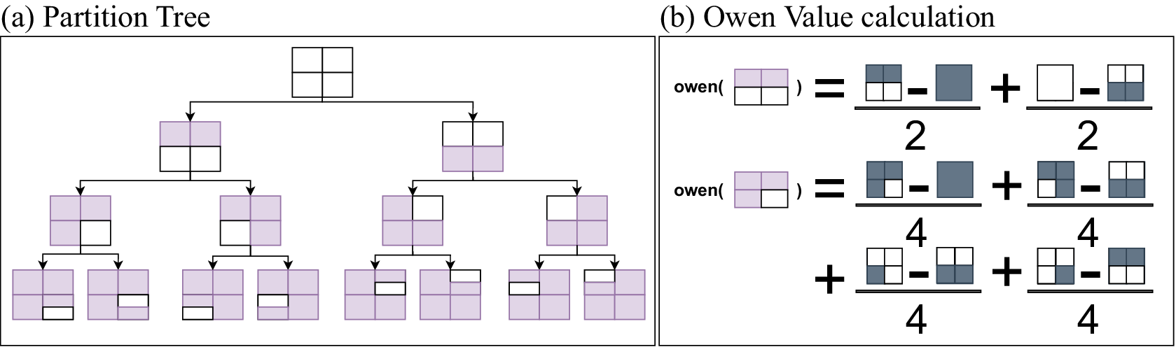
Figure 3. The hierarchy is defined by the partition tree that is generated by recursively splitting the raster. An example partition tree for a single channel, shown to a depth of 4, is given in (a). The white elements indicate the superpixel at that node. The tree continues until the leaf nodes are single (row, col) elements. Owen values (b) are calculated recursively, where each superpixel is evaluated based on comparisons with the elements in its larger group either present or absent.
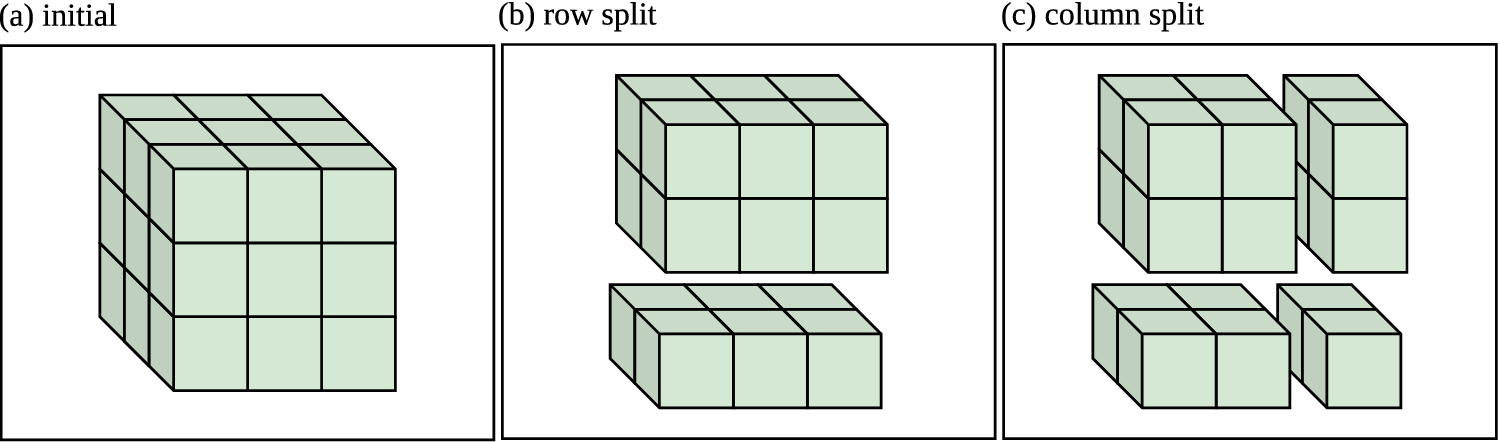
Figure 4. PartitionSHAP’s default scheme for building a partition tree. Given a raster (a), the rows and columns are alternatively halved (nearest integer). (b) demonstrates a row split that divides vertically into two groups. This is followed by a column split (c) dividing each horizontally. This process recursively builds a tree where each group is a node whose children are the two groups formed by splitting it.
Figure 3b illustrates how the Owen values are calculated based on the recursively defined feature hierarchy. First, consider calculating the Owen value of the root node’s left child. This is the superpixel representing the bottom half raster elements. The Owen value is the weighted sum of multiple model evaluations that represent the change in output with and without the superpixel present. The left-hand operation is the difference in model output with no information (all values removed) and with the superpixel’s values added. The right-hand operation is the difference between the model output with all values present and with the superpixel’s values removed. Together, these describe the contribution of the superpixel. Below is the calculation for the bottom-right quadrant superpixel. This example shows more clearly how the hierarchy reduces the number of required computations compared to SHAP. There are four comparisons. First, the difference in output when only the superpixel is present. Then, the output when the group is present but the superpixel is removed. Next, the group is absent, except for the superpixel (and the parent’s sibling is present). Finally, the group is present (sibling absent), and the superpixel is removed. All four evaluations are with respect to the superpixel being evaluated and its parent group. With SHAP, evaluating this bottom-right superpixel would have required evaluating the model with all other quadrants being present or absent. Here, there is no evaluation of the top-left and top-right quadrants since they are not part of the bottom-right feature hierarchy. Since image-based partitioning is performed by arbitrarily splitting the raster elements by the image size, there is no guarantee that the partition hierarchy captures correlated feature groups. Thus, Owen value’s game-theoretic guarantees are violated. Regardless, Hamilton et al. (Reference Hamilton, Lundberg, Zhang, Fu and Freeman2021) applied PartitionSHAP and described the explanations as high quality and outperforming several other XAI methods including Integrated Gradients and LIME. Even without partitioning into optimally correlated clusters, the superpixels contain spatially correlated elements and might cause an appreciable change in the model output compared to a single raster element.
Our main motivation for using PartitionSHAP is efficiency. Shapley-based channel-wise superpixel explanations are feasible because of 2 properties. First, the recursive scheme that lowers the number of required evaluations already described. Second, PartitionSHAP selectively explores the tree to calculate more granular superpixel values based on the magnitude of the Owen values: a superpixel with higher Owen values is prioritized such that its children superpixels will be evaluated before those with lower magnitude values. Given a maximum number of evaluations, PartitionSHAP generates explanations with more influential raster elements at increased granularity. PartitionSHAP divides by rows and columns, and only by channels when at a single (row, col) pixel. Here, we are interested in superpixels inside each of the channels. These represent windows of spatial regions within a single feature map. We added an additional partition scheme option to Lundberg and Lee (Reference Lundberg, Lee, Guyon, Luxburg, Bengio, Wallach, Fergus, Vishwanathan and Garnett2017)’s SHAP software. This partition scheme, illustrated in Figure 5, splits along the channels first, then into superpixels within each channel.
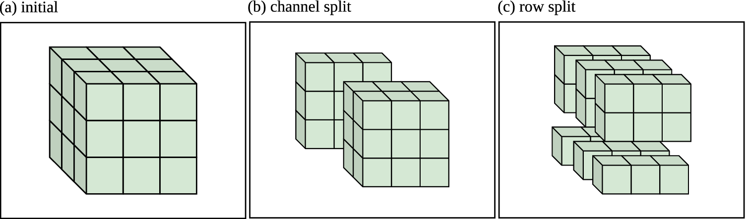
Figure 5. The form channel-wise SuperPixels (CwPS), the input raster (a) is initially divided along the channels. (b) shows the result of a single channel split, dividing the raster into two halves (or, the nearest integer). When the partitioning reaches a single-channel group, it begins recursively diving along the rows and channels as before. (c) shows the result of row splits performed on all three channels.
2.4. Feature importance methods
Feature importance methods quantify the feature’s global influence on model performance. Here we report the change in the Peirce Skill Score (PSS), Heidke Skill Score (HSS), and Clayton Skill Score (CSS). Unlike simpler error metrics (e.g., mean squared error), these measure skill: it is non-trivial to achieve high skill even with highly imbalanced data. Feature importance methods differ mainly in how feature removal is simulated. A trivial example is replacement with random values. Random values could create unrealistic input samples well outside the domain of the training data. The model’s output may reflect the use of unrealistic data rather than properly simulating the removal of that feature (Molnar et al., Reference Molnar, König, Herbinger, Freiesleben, Dandl, Scholbeck, Casalicchio, Grosse-Wentrup and Bischl2020). Alternatively, the replacement value could be randomly selected from that feature’s value in other dataset samples to ensure realistic values. The combination with other features could still be unrealistic, again risking model evaluation with out-of-sample inputs. Molnar et al. (Reference Molnar, König, Herbinger, Freiesleben, Dandl, Scholbeck, Casalicchio, Grosse-Wentrup and Bischl2020) describes feature replacement challenges.
2.4.1. Refitting methods
An alternative is to retrain the model without each feature and measure the performance change (Au et al., Reference Au, Herbinger, Stachl, Bischl and Casalicchio2022). Retraining for each feature requires substantial computing resources which is infeasible for models with high-dimensional inputs. Requiring $ > $
2 h to train, it would take
$ > $
2 h to train, it would take $ > $
786432 h to explain each element of FogNet’s (32, 32, 384)-size raster. Because of training randomness, each should be done multiple times. It is practical to apply refitting to coarser groups such as the 5 physics-based channel groups. Here, we refer to the refitting method as Group-Hold-Out (GHO). While refitting avoids out-of-sample replacement, it does not entirely mitigate feature correlation concerns. If features
$ > $
786432 h to explain each element of FogNet’s (32, 32, 384)-size raster. Because of training randomness, each should be done multiple times. It is practical to apply refitting to coarser groups such as the 5 physics-based channel groups. Here, we refer to the refitting method as Group-Hold-Out (GHO). While refitting avoids out-of-sample replacement, it does not entirely mitigate feature correlation concerns. If features $ x $
and
$ x $
and $ y $
provide strong discriminative information, but are highly correlated with one another, then retraining with only
$ y $
provide strong discriminative information, but are highly correlated with one another, then retraining with only $ x $
or
$ x $
or $ y $
removed might have a negligible impact on model performance. One could imagine retraining the model with each group of features removed, like SHAP, but with combinatorial model retraining. Also, the explanation is technically not for the model originally to be explained since each refitting generates a new model. If each model is learning unique strategies (i.e., many equally valid data associations can predict the target), then it may be misleading to rely on this as an explanation of the specific model.
$ y $
removed might have a negligible impact on model performance. One could imagine retraining the model with each group of features removed, like SHAP, but with combinatorial model retraining. Also, the explanation is technically not for the model originally to be explained since each refitting generates a new model. If each model is learning unique strategies (i.e., many equally valid data associations can predict the target), then it may be misleading to rely on this as an explanation of the specific model.
2.4.2. Permutation feature importance
PFI simulates feature removal with permutation to replace the feature’s values (Breiman, Reference Breiman2001). The following is a summary of PFI to calculate the importance of a single feature $ {x}_i\in X $
where
$ {x}_i\in X $
where $ X $
is the set of all features. For every sample in a set of samples, permute the value of feature
$ X $
is the set of all features. For every sample in a set of samples, permute the value of feature $ {x}_i $
and compute the output with the modified input. This yields a set of model outputs. Then, compute the model performance using a chosen metric (e.g., the loss function). Next, calculate the difference between the model’s original performance and that of the modified input. The mean difference is the importance score. If the model performance drops significantly, then
$ {x}_i $
and compute the output with the modified input. This yields a set of model outputs. Then, compute the model performance using a chosen metric (e.g., the loss function). Next, calculate the difference between the model’s original performance and that of the modified input. The mean difference is the importance score. If the model performance drops significantly, then $ {x}_i $
is considered an important feature. If there is minimal performance change, then
$ {x}_i $
is considered an important feature. If there is minimal performance change, then $ {x}_i $
is either unimportant or has information that is redundant with other features (McGovern et al., Reference McGovern, Lagerquist, Gagne, Jergensen, Elmore, Homeyer and Smith2019).
$ {x}_i $
is either unimportant or has information that is redundant with other features (McGovern et al., Reference McGovern, Lagerquist, Gagne, Jergensen, Elmore, Homeyer and Smith2019).
2.4.3. LossSHAP
LossSHAP is a SHAP variant for feature importance (Covert et al., Reference Covert, Lundberg and Lee2020). Au et al. (Reference Au, Herbinger, Stachl, Bischl and Casalicchio2022) describe Shapley-based XAI algorithms for grouped feature importance. Instead of calculating the average marginal contribution (change in local model output) like SHAP, LossSHAP calculates the average marginal importance (change in global model performance). Like SHAP, the importance is the weighted average of this performance difference, considering all possible combinations of other features being present or absent.
3. Results
Feature importance methods were applied to the entire test dataset (2229 cases). PFI was applied to three feature grouping schemes: channel groups, channels, and channel-wise superpixels (CwSPs). Because of their computational requirements, LossSHAP and GHO were applied only to the 5 channel groups. Feature effect methods were applied to 293 cases taken from both test and validation datasets. This includes all 67 hits, 64 misses, and 78 false alarms, as well as 84 randomly selected correct rejections. The hits and misses are further broken down by fog type. Here, we are most interested in advection fog and the combined category radiation and advection-radiation fog. Unless the phrase radiation and advection-radiation fog is used, radiation fog refers to both radiation and advection-radiation fog because the same mechanism is responsible for the formation of both: radiational cooling. Advection fog is the majority fog case (50 hits, 34 misses). For radiation and advection-radiation fog, there is only 1 hit and 10 misses. SHAP could not be applied to the 384 channels directly due to its complexity, so we applied it only to the 5 channel groups. Figure 6a shows the distribution of the group SHAP values. The most common case (96%) is no fog and although we use a threshold value of .8, the mean value is .048. Thus, the SHAP values overall tend to be quite small for most cases in the test dataset, and Figure 6a shows that the groups all have a similar impact since their SHAP value distributions are similar. Figure 6b shows the distributions of the SHAP values broken out by outcome (hit: 37, miss: 30, correct-reject: 2126, false-alarm: 35). Here we see a different story. G4 plays a bigger role in moving the decision of FogNet towards one of fog. The other four groups also contribute to a decision of fog, but their distributions are very close to each other showing a similar contribution for when the model predicts fog.
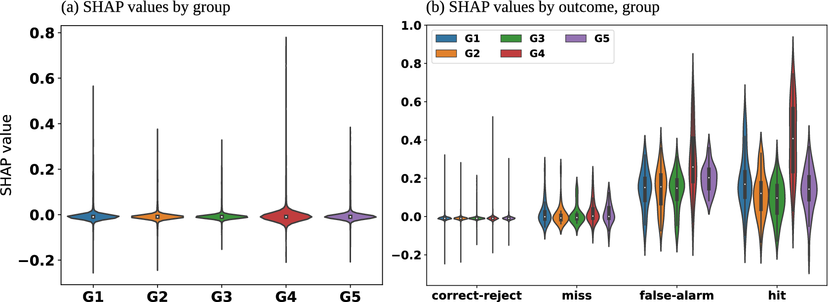
Figure 6. SHAP feature effect results for the 5 groups. SHAP values for each group are calculated for each of the 2228 cases and the violin plots represent the distribution of the SHAP value for those cases. (a) lists all 2228 cases, while (b) aggregates based on the outcome.
CwPS was used to determine superpixel SHAP values. CwPS creates a local explanation and needs to be performed on each sample. Since it is quite slow, we use only 293 FogNet cases (a sample of the correct rejects, plus all the hits, false alarms, and misses) from the validation and test datasets. While Molnar (Reference Molnar2022) generally recommends performing XAI on the test data, we combined it with validation because of the highly imbalanced dataset. Hits and misses are further broken down by fog type, again focusing on advection fog and combined radiation & advection-radiation fog. We hypothesize that FogNet is mainly learning to predict the dominant fog type, advection fog. But we do not know if FogNet is simply applying advection fog strategies to all fog types, or if it is learning different strategies ineffectively.
CwPS yields a high-volume output: 293 explanations of (32, 32, 384)-size SHAP values. We are interested in broadly characterizing the model’s strategies for the outcome categories, so we aggregate local explanations for each outcome. We used three aggregation schemes: spatial-channel, spatial, and channel SHAP values. The spatial-channel aggregations are the sum of the CwPS outputs within each outcome category. While there is some risk of positive and negative SHAP values canceling out, this highlights the dominant sign of the SHAP values. This enables seeing which CwSPs are consistently influential toward or away from the category’s prediction. A cursory manual inspection showed that the relatively high-magnitude SHAP values are confined to a small number of channels. So, we ranked the channels by their maximum absolute superpixel SHAP value as shown in Figure 7. This figure only shows the top-ranked channels that correspond to timestep $ {t}_3 $
which are the 24-h lead time NAM outputs. The decision to highlight
$ {t}_3 $
which are the 24-h lead time NAM outputs. The decision to highlight $ {t}_3 $
channels is because they support a meteorological analysis of the XAI results. Specifically, to examine if the
$ {t}_3 $
channels is because they support a meteorological analysis of the XAI results. Specifically, to examine if the $ {t}_3 $
features that are detected as being important based on XAI techniques correspond to a forecaster’s knowledge of fog conditions which here are predicted for a 24-h lead time. The meteorological interpretation of these figures is included in Section 4.1. All XAI outputs are available online (see Section 5). To highlight influential spatial regions, the SHAP values of each channel were summed at each (row, col) location as shown in Figure 8.
$ {t}_3 $
features that are detected as being important based on XAI techniques correspond to a forecaster’s knowledge of fog conditions which here are predicted for a 24-h lead time. The meteorological interpretation of these figures is included in Section 4.1. All XAI outputs are available online (see Section 5). To highlight influential spatial regions, the SHAP values of each channel were summed at each (row, col) location as shown in Figure 8.
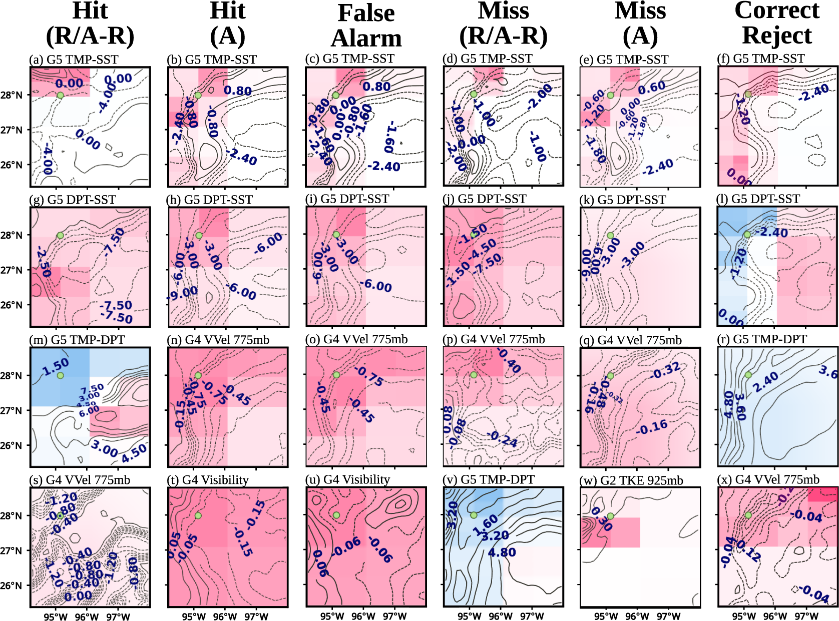
Figure 7. Top $ {T}_3 $
CwPS spatial aggregates, ranked by absolute SHAP. Red (blue) means pushing towards a fog (non-fog) decision. R/A-R is radiation and advection-radiation fog, and A is advection fog. For reference, an outline of the coastline is shown in (w).
$ {T}_3 $
CwPS spatial aggregates, ranked by absolute SHAP. Red (blue) means pushing towards a fog (non-fog) decision. R/A-R is radiation and advection-radiation fog, and A is advection fog. For reference, an outline of the coastline is shown in (w).
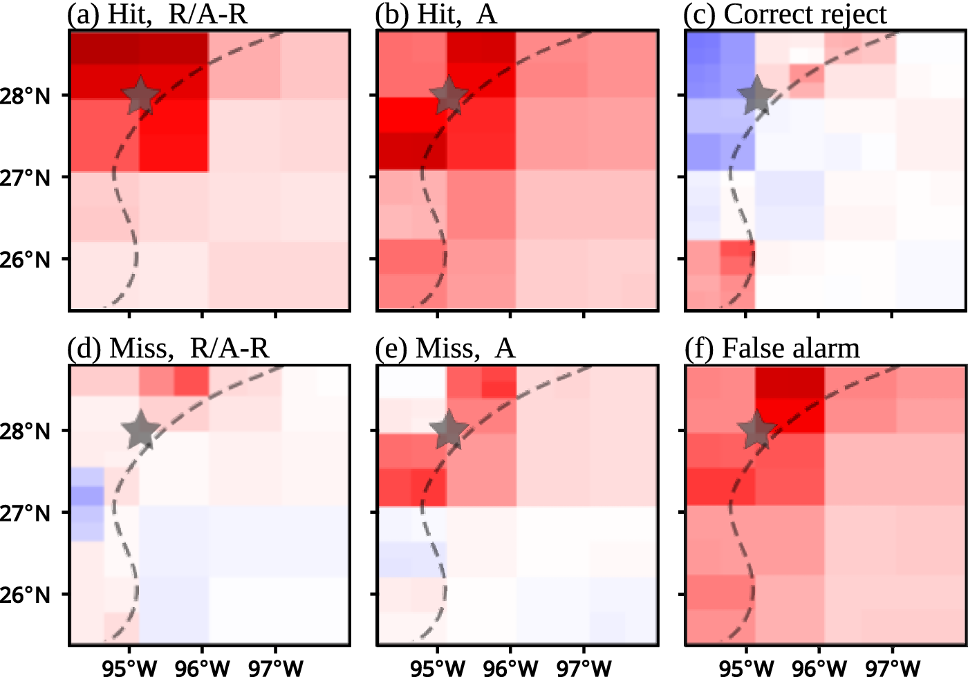
Figure 8. Spatial-channel aggregates of CwPS results are summed along channels to yield 2D explanations. Left of the dotted curve is land and right is water. The star indicates the fog target location (KRAS). Red (blue) means pushing towards a fog (non-fog) decision. R/A-R is radiation and advection-radiation fog, and A is advection fog.
Finally, CwPS outputs were aggregated into 384 channel explanations for each category to highlight influential spatial-temporal variables. By performing XAI at the superpixel level, we expect that some influential features will not be detected because of correlations. To draw out low-magnitude values for comparing the relative channel influence to channel-wise feature importance (Figure 10b,c), we use counting-based aggregation. After ordering channels by the maximum absolute value of their superpixels, we counted the number of occurrences in the top $ N $
channels (Figure 9) Intuitively, if a channel frequently occurs in the top
$ N $
channels (Figure 9) Intuitively, if a channel frequently occurs in the top $ N $
then it suggests that the channel is overall influential. We also counted the number of occurrences of each channel in the bottom
$ N $
then it suggests that the channel is overall influential. We also counted the number of occurrences of each channel in the bottom $ N $
channels. Figure 9a shows that G4 and G5 features are amongst the most influential with respect to radiation and advection-radiation fog for cases where FogNet successfully predicts fog or mist with 1600 meter or less visibility. G4 includes NAM visibility and vertical velocities of 700 mb and below. Negative vertical velocities tend to occur below the 220-meter height level during radiation and advection-radiation fog (Liu et al., Reference Liu, Yang, Niu and Li2011; Dupont et al., Reference Dupont, Haeffelin, Stolaki and Elias2016). G5 includes TMP-DPT, which must be less than 2 degrees Celsius to facilitate saturation necessary for radiation fog, and TMP-SST which modulates fog development; if TMP-SST is negative, an upward-directed sensible heat flux will counteract radiational cooling and either delay fog onset, or prevent fog.
$ N $
channels. Figure 9a shows that G4 and G5 features are amongst the most influential with respect to radiation and advection-radiation fog for cases where FogNet successfully predicts fog or mist with 1600 meter or less visibility. G4 includes NAM visibility and vertical velocities of 700 mb and below. Negative vertical velocities tend to occur below the 220-meter height level during radiation and advection-radiation fog (Liu et al., Reference Liu, Yang, Niu and Li2011; Dupont et al., Reference Dupont, Haeffelin, Stolaki and Elias2016). G5 includes TMP-DPT, which must be less than 2 degrees Celsius to facilitate saturation necessary for radiation fog, and TMP-SST which modulates fog development; if TMP-SST is negative, an upward-directed sensible heat flux will counteract radiational cooling and either delay fog onset, or prevent fog.
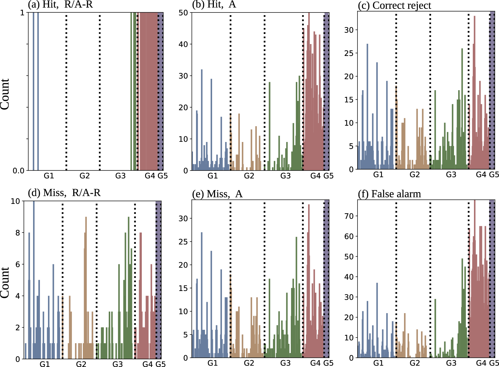
Figure 9. CwPS channel rankings. When summing the superpixel SHAP values, the disproportionate influence of G4 and G5 channels causes channels in other groups to virtually disappear. We instead ranked channels based on the number of times that a channel appears within the top 50 channels.
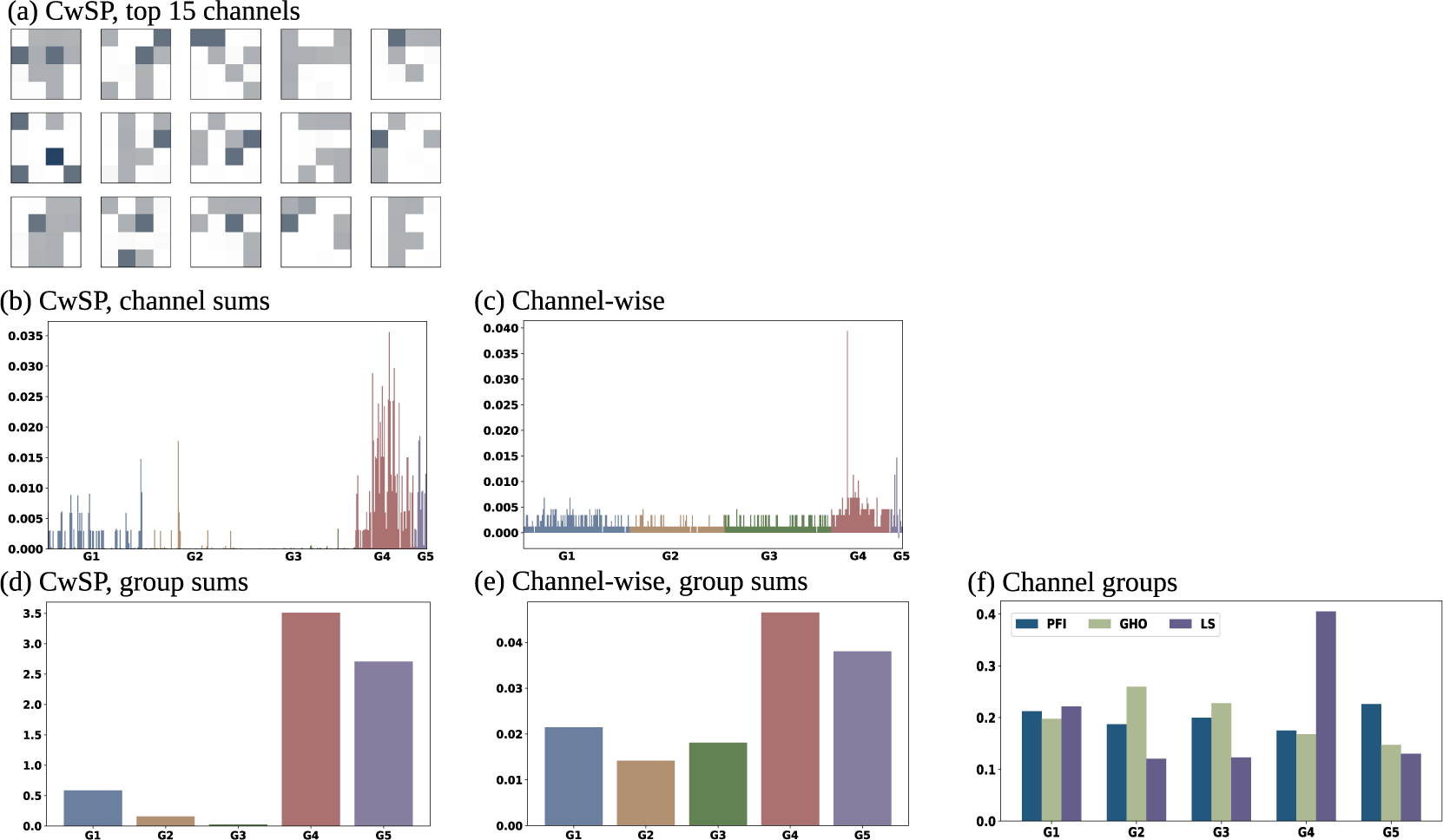
Figure 10. Feature importance at three granularities. To compare consistency across grouping schemes, the more granular explanations are aggregated into coarser ones. (a) Each column corresponds to the grouping scheme, and each row corresponds to an aggregation granularity. (a) shows the top 15 channels based on PFI performed on CwSP (left-to-right, top-to-bottom). (b and c) Showing individual features. (d and e) Showing the prior row aggregated by group, and e shows methods used on the five groups.
Three feature importance methods were applied to three grouping schemes. Some groups may be more sensitive to the grouping scheme. The sensitivity comparison may suggest that we can use the coarser explanations for a subset of groups that show greater consistency, but it is not straightforward to directly compare the importance values of different groups. At each level of granularity, we sum PFI values into the coarser groups to compare rankings. Another sanity check is PFI’s consistency with GHO and LS. The latter are expected to be more robust to correlation and out-of-sample inputs. If PFI performed on channel groups reaches similar relative importance rankings to the others, then we have additional confidence in using the (consistent) more granular PFI explanations. Figure 10 gives all feature importance results, aligned in a table to assist comparison. Each column corresponds to the grouping scheme used to generate importance values. Column 1 is CwSPs, column 2 is channels, and column 3 is channel groups. Rows correspond to the aggregation level. The top of each column is without any aggregation. The second row is for channels, and the third is for channel groups.
4. Discussion
We use Figure 10 to analyze sensitivity to groups. Figure 10a shows PFI applied to CwSP features (using PSS). To assess the consistency of CwSP explanations to channel-wise, Figure 10b shows the sum of absolute PFI values in each channel. This can be directly compared to Figure 10c, the PFI values computed when PFI is applied directly to channel-wise features. When considering summed superpixels (Figure 10b), important channels tend to be within G4 and G5. The top channel occurs in G4: Vertical velocity at 950mb, $ {t}_1 $
. Sparse G1 and G2 channels have some importance, with practically no importance for G3. When considering individual channels using PFI, Figure 10c, we observe considerable influence from G4 and G5 as we did with the CwSP-based results in Figure 10b. Again, Vertical velocity at 950mb,
$ {t}_1 $
. Sparse G1 and G2 channels have some importance, with practically no importance for G3. When considering individual channels using PFI, Figure 10c, we observe considerable influence from G4 and G5 as we did with the CwSP-based results in Figure 10b. Again, Vertical velocity at 950mb, $ {t}_1 $
in G4 has the highest importance. Otherwise, the exact rank order does differ between CwSP and channel-wise explanations. Two differences stand out between Figures 10b and 10c. In the channel-wise results (Figure 10c), two G4 and G5 channels have such high importance that others are suppressed. This does not occur in the CwSP results (Figure 10b), where some channels in G1 and G2 are shown to be comparable to G4 and G5 channels. Another difference is that in the CwSP results (Figure 10b), G3 channels are considered to have practically no importance while in channel-wise results (Figure 10c), G1–G3 are approximately uniform in average importance. At the superpixel level, importance means that the specific superpixel influenced the model. At the channel level, importance scores mean that at least some spatial region within the variable had an influence. When a channel is important according to Figure 10c but not in Figure 10b, it may suggest that the model is learning a large-scale feature in that channel. By comparing Figures 10b and 10c, we get some insight into the scale of the features learned. It is also possible that the difference is due simply to random permutations, but there is evidence that suggests that, at least to some extent, the difference between Figures 10b and 10c reflects the scale of the learned features. In general, the importance scores are smaller when summing superpixels which suggests that the importance becomes diluted at the smaller scale. Also, the dilution is prominent in G1–G3 which are vertical profiles where we expect granular features to have little fog information.
$ {t}_1 $
in G4 has the highest importance. Otherwise, the exact rank order does differ between CwSP and channel-wise explanations. Two differences stand out between Figures 10b and 10c. In the channel-wise results (Figure 10c), two G4 and G5 channels have such high importance that others are suppressed. This does not occur in the CwSP results (Figure 10b), where some channels in G1 and G2 are shown to be comparable to G4 and G5 channels. Another difference is that in the CwSP results (Figure 10b), G3 channels are considered to have practically no importance while in channel-wise results (Figure 10c), G1–G3 are approximately uniform in average importance. At the superpixel level, importance means that the specific superpixel influenced the model. At the channel level, importance scores mean that at least some spatial region within the variable had an influence. When a channel is important according to Figure 10c but not in Figure 10b, it may suggest that the model is learning a large-scale feature in that channel. By comparing Figures 10b and 10c, we get some insight into the scale of the features learned. It is also possible that the difference is due simply to random permutations, but there is evidence that suggests that, at least to some extent, the difference between Figures 10b and 10c reflects the scale of the learned features. In general, the importance scores are smaller when summing superpixels which suggests that the importance becomes diluted at the smaller scale. Also, the dilution is prominent in G1–G3 which are vertical profiles where we expect granular features to have little fog information.
The difference between CwSP and channel-wise is further emphasized when summing both to the group level as shown in Figures 10d and 10e. Comparing G4 and G5, we observe that their relative importance is consistent. Comparing G1–G3, importance drops considerably from the transition to the more granular CwSPs. Figure 10f shows PFI, along with LS and GHO, applied directly to the channel groups. Using this grouping scheme, the importance of the groups is more uniform. G4 is now the least important group, instead of the most as it is in Figures 10d and 10e. The manner in which G1–G3 drops in importance as the granularity of the partitions increases suggests that the model is learning large-scale patterns. G4 and G5 are less influenced by the change in granularity, suggesting smaller-scale learned features so that granular perturbations of the model still influence model performance.
There is evidence that differences are in part due in part to the scale of the learned features. It is encouraging that XAI provides evidence that the model can learn large-scale features that take advantage of spatial-temporal relationships across the channels. We argue that our PFI interpretation relies heavily on having performed XAI on three different feature groups. If we were to compare CwSPs to channel groups (skipping channels), we would have less confidence in the interpretation that the discrepancy between them reflects characteristics of the learned patterns. Since we would have only the 2 examples, we would be less confident that the difference is not merely due to randomness or method inaccuracy. But by including the channel-wise output, we observe G1–G3 reduce in importance in relation to the increase in granularity, which increases our confidence that the explanations reflect reality. The explanation is not entirely satisfying: we can see that G1 is important but we do not know which parts of the raster compose its learned features. Even if we get the sense that, broadly, across-channel relationships are involved, we don’t know if these are spatial, temporal, or spatial-temporal. With the present computational efficiencies, it would be too computationally complex to perform PFI on all combinations of channels, much less all possible voxels within the raster. Another concern is the overall accuracy of PFI itself. In addition to PFI, Figure 10f includes group results using 2 other XAI methods: GHO and LS. While we are minimally concerned about the differences in exact magnitudes between the three methods, we are concerned with their disagreement in the group rankings amongst themselves and the aggregation of the CWSP and channel-wise PFI results.
Some disagreement with GHO is expected since importance is based on refitting models so that each has the chance to learn other relationships within the data in the absence of the removed group. This is quite different from the other two XAI methods that are based on models that had access to the removed group during training. Even if a particular model placed high emphasis on particular features, that does not mean that other features could not be used instead to achieve similar performance. Compared with the PFI and LS, the GHO results show relative uniformity in the importance of the groups. This suggests that the model is still able to learn fog prediction strategies by using different feature relationships.
The comparisons lead to concerns about the disagreement between PFI and LS. First, the game theoretic guarantees suggest that SHAP-based methods might have greater reliability. Second, by averaging over the marginal distribution, LS importance scores are based on several comparisons of perturbed features. Repeating PFI multiple times, high variance is observed for CwSP results but not channel-wise. The output of each CwSP PFI repetition does not significantly alter the ranking of the channels when summing the importance scores. However, the distribution of those scores among the superpixels is inconsistent. Each complete repetition of CwSP PFI requires 80 h of computation, so we are unable to run extensive repetitions with present computational capabilities. Among the three runs, we observe little similarity among the maps. Since their summed channel-wise rankings are relatively consistent, we choose to analyze the top channels as determined by CwSP PFI to that of channel-wise PFI.
Is it of interest to compare the PFI values from Figure 10 to the top channels based on CwPS shown in Figure 9. The overall shape of the channel rankings is not unlike that in Figure 10c. Except that every G5 channel is consistently of very high influence according to CwPS. Recall that feature effect includes when the model uses a feature for incorrect decisions. Comparing Advection fog hits to misses, G5 features have a very high influence in both. This suggests that G5 channels are being used both for decisions that improve and decrease performance. The net effect could be a lowered importance compared to G4. G4 values have more influence on the hits than misses which would increase G4 importance.
4.1. Meteorological interpretation
The following is an analysis of the foregoing XAI output from a meteorological perspective. In particular, we assess the extent to which FogNet features with high feature effect and importance account for the primary mechanisms responsible for, or the environmental conditions associated with, fog development. In addition, we use feature effect output to assess the utility of various features. Finally, we analyze feature importance output to assess the relative importance of individual features versus feature groups with respect to fog prediction. We believe that XAI output which (1) identifies features with high feature effect, or features and feature groups with high feature importance, that account for fog generation mechanisms and/or environmental conditions associated with fog, and which (2) identifies features with high utility, demonstrate trustworthiness.
First, we consider feature effect output. To assess feature utility, we adopt the XAI analysis strategy of Clare et al. (Reference Clare, Sonnewald, Lguensat, Deshayes and Balaji2022), which suggests that a feature, used to develop an ML model, is useful if it pushes the model in a direction that was actually predicted. Applying this concept to FogNet means that if a given FogNet feature pushes FogNet toward a positive fog prediction, and FogNet actually predicted fog, or if the feature pulls FogNet away from a positive fog prediction (toward a no-fog prediction) and FogNet predicted no-fog, then that feature was helpful to FogNet (possess utility). Applying this logic to the 24 feature maps in Figure 7 reveals that in 20 ( $ \approx $
83%) of these feature maps, the feature was helpful to FogNet: When FogNet predicted fog (Hit, False Alarm), the feature pushed FogNet toward a prediction of fog (red color coincident with target location represented by the green dot), and when FogNet predicted no-fog (Miss, Correct Rejection), the feature pushed FogNet toward a prediction of no-fog (blue color coincident with target location). One of the 20 useful feature maps is Figure 7b: the feature TMP-SST pushes FogNet toward a prediction of fog at the target (red color coincident with target location) for cases when FogNet predicts fog (Hit). Another useful feature map is Figure 7l: the feature DPT-SST pushes FogNet toward a no-fog prediction at the target (blue color coincident with the target location) for cases when FogNet predicts no-fog (Correct Rejection). In the remaining 4 features maps (Figures 7m,r,s,v), the feature was not helpful to FogNet. The preponderance of useful feature maps adds to the trustworthiness of FogNet. Trustworthiness is also apparent when performing a 2D spatial analysis of a given feature as a function of prediction outcome. Note in Figure 7 that the same feature (the 2-meter temperature minus sea/land surface temperature, or TMP-SST) appears in the highest-ranked row based on absolute maximum SHAP value (Figures 7a–f). Thus, we can perform an analysis strategy similar to that of Lagerquist (Reference Lagerquist2020), whereby 2D feature maps of the same feature are analyzed as a function of FogNet fog prediction outcome (Hit, False Alarm, Miss, Correct Rejection) and fog type (radiation versus advection fog). With respect to cases when advection fog occurred (Figures 7b and 7e), note the region of TMP-SST
$ \approx $
83%) of these feature maps, the feature was helpful to FogNet: When FogNet predicted fog (Hit, False Alarm), the feature pushed FogNet toward a prediction of fog (red color coincident with target location represented by the green dot), and when FogNet predicted no-fog (Miss, Correct Rejection), the feature pushed FogNet toward a prediction of no-fog (blue color coincident with target location). One of the 20 useful feature maps is Figure 7b: the feature TMP-SST pushes FogNet toward a prediction of fog at the target (red color coincident with target location) for cases when FogNet predicts fog (Hit). Another useful feature map is Figure 7l: the feature DPT-SST pushes FogNet toward a no-fog prediction at the target (blue color coincident with the target location) for cases when FogNet predicts no-fog (Correct Rejection). In the remaining 4 features maps (Figures 7m,r,s,v), the feature was not helpful to FogNet. The preponderance of useful feature maps adds to the trustworthiness of FogNet. Trustworthiness is also apparent when performing a 2D spatial analysis of a given feature as a function of prediction outcome. Note in Figure 7 that the same feature (the 2-meter temperature minus sea/land surface temperature, or TMP-SST) appears in the highest-ranked row based on absolute maximum SHAP value (Figures 7a–f). Thus, we can perform an analysis strategy similar to that of Lagerquist (Reference Lagerquist2020), whereby 2D feature maps of the same feature are analyzed as a function of FogNet fog prediction outcome (Hit, False Alarm, Miss, Correct Rejection) and fog type (radiation versus advection fog). With respect to cases when advection fog occurred (Figures 7b and 7e), note the region of TMP-SST $ \ge $
0 (weakly positive) just offshore; this pattern is typical of advection fog events along the Middle Texas coast. The condition TMP-SST
$ \ge $
0 (weakly positive) just offshore; this pattern is typical of advection fog events along the Middle Texas coast. The condition TMP-SST $ > $
0 implies a downward-directed near-surface sensible heat flux to the sea, and thus a corresponding heat loss or cooling of the near-surface air temperature to the dew point temperature resulting in saturation and subsequent fog development (Huang et al., Reference Huang, Liu, Huang, Mao and Bi2015; Lakra and Avishek, Reference Lakra and Avishek2022), subject to a cloud drop-size distribution that favors the extinction of light and subsequent visibility reduction (Twomey, Reference Twomey1974; Koračin et al., Reference Koračin, Dorman, Lewis, Hudson, Wilcox and Torregrosa2014). Thus, the spatial pattern of a feature with high feature effect successfully identified an environmental condition (and associated mechanism) conducive to fog. Finally, spatial aggregates of CwPS results from all features reveal that when FogNet correctly predicts both radiation and advection fog (Figures 8a,b), the strongest influential region (darkest red color) is near the target (KRAS). This is consistent with the domain knowledge which posits that the formation and dissipation of fog are controlled by local factors (Lakra and Avishek, Reference Lakra and Avishek2022). However, non-local factors are also important. In particular, the larger scale wind pattern can influence the intensity of marine advection fog (Lee et al., Reference Lee, Lee, Park, Chang and Lee2010; Lakra and Avishek, Reference Lakra and Avishek2022) (which may account for the lighter-colored red over the waters in Figure 8b). The use of XAI output to confirm expert knowledge regarding the scale of fog development adds trustworthiness.
$ > $
0 implies a downward-directed near-surface sensible heat flux to the sea, and thus a corresponding heat loss or cooling of the near-surface air temperature to the dew point temperature resulting in saturation and subsequent fog development (Huang et al., Reference Huang, Liu, Huang, Mao and Bi2015; Lakra and Avishek, Reference Lakra and Avishek2022), subject to a cloud drop-size distribution that favors the extinction of light and subsequent visibility reduction (Twomey, Reference Twomey1974; Koračin et al., Reference Koračin, Dorman, Lewis, Hudson, Wilcox and Torregrosa2014). Thus, the spatial pattern of a feature with high feature effect successfully identified an environmental condition (and associated mechanism) conducive to fog. Finally, spatial aggregates of CwPS results from all features reveal that when FogNet correctly predicts both radiation and advection fog (Figures 8a,b), the strongest influential region (darkest red color) is near the target (KRAS). This is consistent with the domain knowledge which posits that the formation and dissipation of fog are controlled by local factors (Lakra and Avishek, Reference Lakra and Avishek2022). However, non-local factors are also important. In particular, the larger scale wind pattern can influence the intensity of marine advection fog (Lee et al., Reference Lee, Lee, Park, Chang and Lee2010; Lakra and Avishek, Reference Lakra and Avishek2022) (which may account for the lighter-colored red over the waters in Figure 8b). The use of XAI output to confirm expert knowledge regarding the scale of fog development adds trustworthiness.
Trustworthiness is also apparent in feature importance output. Table 1 depicts the top 15 PFI features ranked separately by the channel-wise (Cw) and CwSP methods, as a function of the following 3 separate performance metrics: PSS, HSS, and the CSS. All three performance metrics measure skill (accuracy normalized by a standard, such as accuracy associated with random forecasts). PSS and CSS also measure value (incremental benefits to users of the forecasts). Using metrics that assess both forecast skill and value, we broaden the list of features that possess high feature importance, thus allowing for the discovery of a more comprehensive list of the features most responsible for FogNet’s performance. Many of the features in Table 1 account for environmental conditions and/or mechanisms conducive to fog development. The following are a few examples: Note that the feature list in Table 1 includes the features TMP-SST, the dew point depression (TMP-DPT), vertical velocities (VVEL) in the 975 to 700-mb layer, and the specific humidity at the 2-meter height (Q surface). The mechanism implied by TMP-SST was described earlier. The saturation or near saturation of near-surface water vapor (low values of TMP-DPT) is necessary for fog development (Gultepe et al., Reference Gultepe, Tardif, Michaelides, Cermak, Bott, Bendix, Muller, Pagowski, Hansen, Ellrod, Jacobs, Toth and Cober2007; Lakra and Avishek, Reference Lakra and Avishek2022). Advection and radiation fogs are associated with larger-scale subsidence/negative VVEL values (Huang et al., Reference Huang, Huang, Liu, Yuan, Mao and Liao2011; Yang et al., Reference Yang, Liu, Ren, Xie, Zhang and Gao2017; Mohan et al., Reference Mohan, Temimi, Ajayamohan, Nelli, Fonseca, Weston and Valappil2020). Sufficient near-surface moisture (high Q surface values) is essential for fog development (Gultepe et al., Reference Gultepe, Tardif, Michaelides, Cermak, Bott, Bendix, Muller, Pagowski, Hansen, Ellrod, Jacobs, Toth and Cober2007; Lakra and Avishek, Reference Lakra and Avishek2022). The trustworthiness of FogNet based on feature importance XAI output is also demonstrated by the relative importance of individual features/channels or feature groups. Consider the following discussion of G3 importance, which contains channels TMP and RH at 2 meters, and from 975-mb to 700-mb (at 25-mb increments). Note that Figure 10 depicts the relative importance of features and feature groups. A comparison between the coarse channel grouping methods (Figure 10f) to the more granular CwSP scheme (Figure 10b), reveals a major difference in feature importance with respect to G3. Note the near-zero importance of individual G3 features yet the significant importance of G3 as a whole. This disparity is understandable from a meteorological perspective. Each TMP channel has no significant relationship to fog development. However, the increase in TMP with height (temperature inversion) is critical to fog development (Koračin et al., Reference Koračin, Dorman, Lewis, Hudson, Wilcox and Torregrosa2014; Huang et al., Reference Huang, Liu, Huang, Mao and Bi2015; Price, Reference Price2019). Except for the 2-meter relative humidity (RH), individual RH channels from 975-mb to 700-mb are less important to fog. Yet, an environment characterized by a thin moist layer near the surface followed by dry air aloft (rapid decrease in RH with height) would be conducive to radiation fog (Koračin et al., Reference Koračin, Dorman, Lewis, Hudson, Wilcox and Torregrosa2014; Huang et al., Reference Huang, Liu, Huang, Mao and Bi2015; Mohan et al., Reference Mohan, Temimi, Ajayamohan, Nelli, Fonseca, Weston and Valappil2020). This explains the negligible feature importance of individual G3 channels in Figure 10b and the much stronger importance of the G3 group in Figure 10f. These results are consistent with those found in Kamangir et al. (Reference Kamangir, Krell, Collins, King and Tissot2022), where XAI output revealed the collective importance of G3. Thus, XAI results reveal that FogNet recognizes the physical relationship between the vertical profile of TMP and RH and fog development.
Table 1. Top 15 $ {t}_3 $
channels ranked with channel-wise (Cw) and CwSP schemes
$ {t}_3 $
channels ranked with channel-wise (Cw) and CwSP schemes
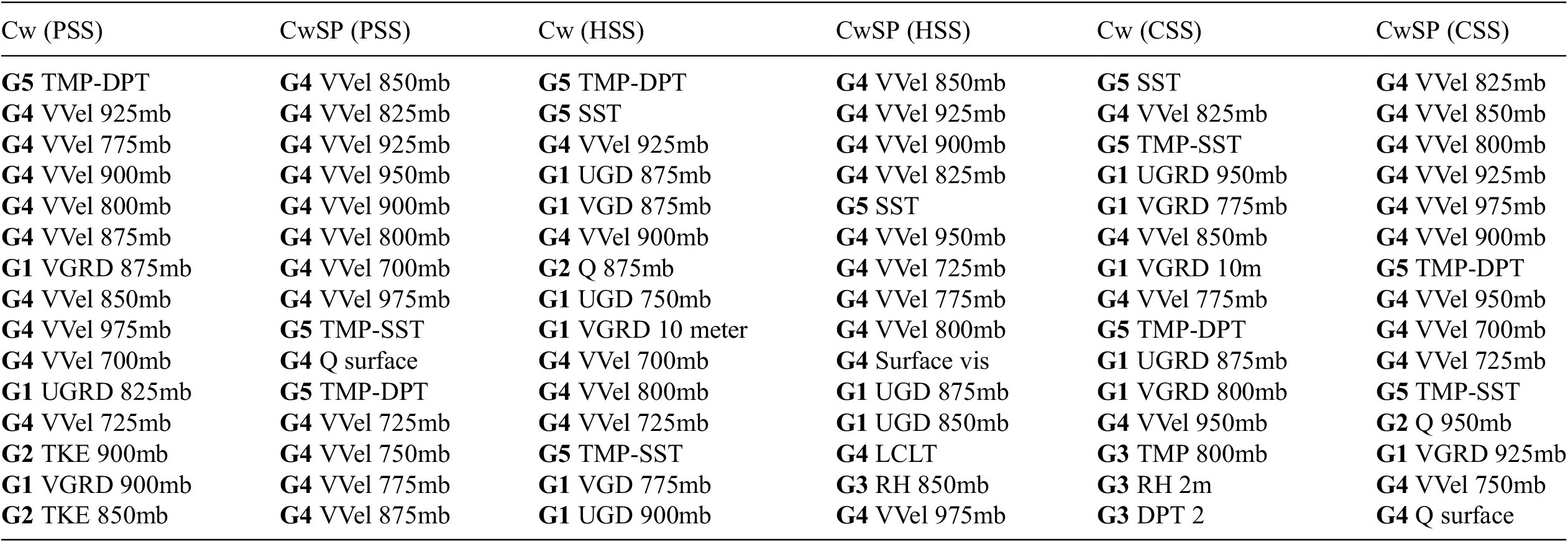
XAI results also demonstrate a reduction in trustworthiness. FogNet performed superior to the HREF ensemble prediction system, yet performed poorly during radiation fog cases (Kamangir et al., Reference Kamangir, Collins, Tissot, King, Dinh, Durham and Rizzo2021). XAI output provides insight into why FogNet performed poorly with respect to radiation fog. Note from Figures 7b (test/validation dataset advection fog Hit cases) and 7c (test/validation dataset False Alarm instances) that the TMP-SST pattern associated with False Alarms is similar to that from the corresponding Hit feature map in that the weakly positive values just offshore are retained. Since the vast majority of fog cases were of the advection fog type, we speculate that in each instance in the testing set, FogNet is essentially generating a prediction based primarily on the patterns it learned from advection fog cases in the training/validation dataset. Further, although FogNet recognized the link between the surface and 975-mb temperature inversion and fog development as mentioned earlier, FogNet may have been unable to develop a more effective radiation fog strategy due to the inability to account for processes within surface to 975-mb sublayers critical to radiation fog development (Liu et al., Reference Liu, Yang, Niu and Li2011; Price, Reference Price2019). The reliance on an advection fog pattern to predict all fog types, and the probable incompleteness of the feature set with respect to radiation fog prediction, reflects lower trustworthiness in the use of FogNet by operational meteorologists to predict fog of types other than advection fog. Possible solutions to this class imbalance problem (number of radiation versus advection fog cases in addition to fog versus no-fog) include data augmentation, implementation of a multi-class target where each class is a separate fog type, and the incorporation of additional features strongly related to radiation fog.
In summary, XAI results suggest that the FogNet feature set demonstrates utility, identifies features (and 2D feature map patterns) that contribute to environmental conditions and mechanisms critical to fog development, and adds credence to the knowledge that fog is very often a locally-driven phenomenon, yet also influenced by non-local factors. Further, an assessment of feature importance as a function of granularity provides additional insights, including FogNet’s ability to identify the importance of the vertical structure of certain features to fog development. Finally, XAI provides a plausible explanation for why FogNet performed poorly with respect to radiation cases. These results reveal the power of XAI analysis in assessing model strengths and weaknesses and thus allow for the identification of solutions to improve model performance and trustworthiness. Although the foregoing analyses pertain to FogNet, the XAI feature effect and importance methods used in this study, and the techniques to analyze XAI output in this section, can be applied to any ML model developed to predict atmospheric phenomena and trained on a feature set that represents the 3D environment. We recommend the type of analysis performed by Clare et al. (Reference Clare, Sonnewald, Lguensat, Deshayes and Balaji2022), which can assess the utility of the input feature set based on XAI feature effect contribution on a 2D feature map, and the analysis strategy of Lagerquist (Reference Lagerquist2020), which allows for an assessment of the 2D spatial patterns of a particular highly influential feature as a function of model prediction outcome; the patterns can be compared to the expected pattern based on domain knowledge/expertise to assess model trustworthiness. Furthermore, the spatial aggregation of CwPS results depicts the implied spatial scale(s) of the primary mechanism(s) responsible for the target, which can be compared to the expected scale(s) based on domain knowledge. Finally, to the extent that model architecture includes features organized in groups, an assessment of feature importance as a function of granularity can allow the researcher to assess whether individual features or corresponding feature groups contribute the most to model performance, which in turn forces the expert analyst to identify the physical reasoning for the contribution differential; the model’s ability to recognize physical relationships between model features and the corresponding target adds to model trustworthiness.
5. Conclusions and Future Work
We investigated a complex geoscience model using XAI methods applied to three partitioning schemes and observed some inconsistency among the explanations (Figure 10). Based on channel groups, G3 features are important. CwPS results, however, suggest minimal influence. We argue that each partition scheme asks a different question to the model, and comparing them reveals insights not possible with a single explanation. G3 is the lower atmospheric moisture and temperature information: 3D profile characteristics that are correlated with fog. The PFI results demonstrate that the importance of G3 data rapidly decreases as we increase the granularity of the feature groups. This suggests that the model is learning large-scale features in G3, which was the goal. Groups G4 and G5 are important even at the most granular level. This allows us to study which regions are used to make predictions in those groups. Without the multi-scale feature group experiments, we could be misled into thinking that G1–G3 are not important because their CwSP-based explanations show very little importance or effect.
A major takeaway is that grouping schemes can be a pitfall for model interpretation, but that disagreements should be understood based on how that grouping scheme probes the model. Here, CwSP results suggest that we could redesign FogNet without G3 (Figure 10b), but we also observe that removing G3 would reduce performance considerably (Figure 10f). This discrepancy could lead users to distrust XAI and avoid using it. Instead, XAI outputs should be carefully interpreted based on how that method and feature group probe the model: each explanation is an answer to a question asked by the XAI method. CwSP-based PFI results should not be considered as a single summary of each superpixel’s importance. Instead, the results are narrowly defined as the importance of isolated superpixels. So, the presence of high-ranking G4 and G5 features concentrated around the target location suggests that local information is used, but the lack of importance for others does not mean that they are unimportant: they may be part of larger-scale patterns. We observe G3’s importance diminishes as the features become more granular, suggesting that FogNet learned 3D features. Our results emphasize that complex geoscience models should be investigated using XAI on multiple grouping schemes because each reveals different model characteristics and method disagreement also provides information about the learned strategies.
We also demonstrated aggregating local into global explanations. Global explanations may not provide sufficient insights to describe models of nonlinear systems or with highly imbalanced classes since they give a single explanation that averages out local characteristics. So we may learn very little about what features drive the model’s decision-making for events like fog since the majority of cases are correct rejections. This is illustrated when comparing Figures 6a to 6b. In the former, the dot represents a single global summary of the feature’s importance. A global explanation suggests that groups $ \sim $
equally affect the model. But, recall that the vast majority of cases are correct rejects. Figure 6b shows that the relative effect of each group differs depending on the model outcome. When the model predicts fog (hits and false alarms), G4 strongly pushes the model towards a fog decision. Local explanations are more informative, but it is challenging to extract patterns from, for example, SHAP values for every sample. Here, we demonstrate that practitioners can aggregate local explanations in various ways to explore the model. We recommend visualizing the set of local explanations in various ways.
$ \sim $
equally affect the model. But, recall that the vast majority of cases are correct rejects. Figure 6b shows that the relative effect of each group differs depending on the model outcome. When the model predicts fog (hits and false alarms), G4 strongly pushes the model towards a fog decision. Local explanations are more informative, but it is challenging to extract patterns from, for example, SHAP values for every sample. Here, we demonstrate that practitioners can aggregate local explanations in various ways to explore the model. We recommend visualizing the set of local explanations in various ways.
We showed that models relying on complex rasters may be sensitive to the choice of grouping scheme. We assumed that coarser groups produce more accurate explanations and that PFI’s consistency with GHO and LossSHAP’s ranking order indicates accurate relative feature importance from PFI. But this cannot be confirmed without ground truth attribution. There has been some research in developing XAI benchmarks: models with ground truth explanations for quantitatively ranking XAI methods. Mamalakis et al. (Reference Mamalakis, Ebert-Uphoff and Barnes2022) developed a technique for building models where the attribution of each feature toward the output can be directly calculated. This research targets geoscience applications using gridded data. We are currently working on extending this research for high-dimensional, multi-channel raster data. To investigate the grouping schemes, we are experimenting with the influence of the strength of the correlation among grid cells. The goal is to develop strategies for grouping XAI that can be verified with known attributions.
Author contribution
Conceptualization: E.K., H.K., W.C., P.T., S.K.; Methodology: E.K., H.K., W.C., P.T., S.K.; Data curation: H.K.; Data visualization: E.K., S.K.; Writing original draft: E.K., H.K., W.C., P.T., S.K.; All authors approved the final submitted draft.
Competing interest
The authors declare no competing interests exist.
Data availability statement
The FogNet input predictors include NAM NWP model output and the MUR SST analysis product, both of which are in the public domain. FogNet data combines the 12-km NAM output that is archived in grib2 format at https://www.nco.ncep.noaa.gov/pmb/products/nam (NOAA, 2006) with the Analyzed SST available as a netCDF archive at https://coastwatch.pfeg.noaa.gov/erddap/griddap/jplMURSST41.html (NOAA, 2020). The predictors and targets used in this study are archived at the FogNet data share server: https://gridftp.tamucc.edu/fognet/datashare/archive/datasets/ (Krell et al., Reference Krell, Kamangir, Collins, King and Tissot2022a).
FogNet is available at https://github.com/conrad-blucher-institute/FogNet (Krell et al., Reference Krell, Kamangir, Collins, King and Tissot2023). It includes all XAI methods and analysis except for CwPS which is instead implemented as a modification to the SHAP Python package by (Lundberg and Lee, Reference Lundberg, Lee, Guyon, Luxburg, Bengio, Wallach, Fergus, Vishwanathan and Garnett2017) that is available as a fork of the SHAP repository: https://github.com/conrad-blucher-institute/shap (Krell et al., Reference Krell, Kamangir, Collins, King and Tissot2022b). xai-raster-vis-tools, available at https://github.com/conrad-blucher-institute/xai-raster-vis-tools, is another software repository used in this research that contains several scripts for aggregating and visualizing raster XAI outputs (Krell et al., Reference Krell, Kamangir, Collins, King and Tissot2022c). All the software repositories developed as part of the FogNet project (FogHat, FogNet, xai-raster-vis-tools, and partitionshap-multiband-demo) as well as the data and scripts archived on the FogNet data share server (Krell et al., Reference Krell, Kamangir, Collins, King and Tissot2022a) are released under a Creative Commons 0 1.0 Universal license. The only exception is the SHAP fork containing CwPS since it retains the MIT license used by the original SHAP repository.
Ethics statement
The research meets all ethical guidelines, including adherence to the legal requirements of the study country.
Funding statement
This research was supported by grants from the National Science Foundation (2019758) and the National Science Foundation (1828380).


 Open access