


Introduction
When predicting the durability of radioactive-waste repositories and the stability of the surrounding bedrock during future periods of glaciation, it is essential to model the behaviour and characteristics of groundwaters driven by permafrost related to continental ice sheets (e.g. Boulton and others, 1996). For example, Bath and others (1996) considered hydrogeological models in deducing how the groundwater system might have responded to changing climate, specifically with respect to glaciation. Certes and others (1996) considered the transport of radionuclides due to groundwaters driven by permafrost during glaciation cycles, while Delisle (1996a) developed a numerical model for permafrost growth and decay. King-Clayton and others (1996) presented a model for predicting potential changes in various climatic, stress, hydraulic and hydrochemical parameters over approximately the next 130 000 years when evaluating the future behaviour of a deepdepository for spent fuel.
Like any other theoretical model, these also require testing using our current knowledge of permafrost and groundwater behaviour associated with existing and recent glaciers. However, it is relatively difficult to obtain information on these parameters. In practice it can be done indirectly, for example, by observing bedrock and soil in terrains that have been covered by glacier ice (e.g. Delisle, 1996b; Glynn and Voss, 1996; Ivanovich and others, 1996). Direct observations can be made by drilling through the ice (e.g. Paterson, 1994, and references therein) and permafrost (e.g. Gold and Others, 1973). However, the indirect methods are relatively uncertain, while drilling is expensive and slow and thus cannot provide extensive coverage.
A relatively rapid and economic way is to analyze the variations of permafrost geophysically using electromagnetic measurements to define the conductivity variations within and beneath the permafrost. Hoekstra and McNeill (1973) give a summary of resistivities of various soil and rock types and conclude that there is approximately a factor of 10 between the resistivity of frozen (≈ −10°C) and unfrozen (≈1° soil and rock. The resistivity values also differ between various rock and soil types, which thus can be used for determining lithological and soil variations in the permafrost. Sinha (1975, 1977), Daniels and others (1976) and Sinha and Stephens (1983) considered the theoretical background and gave examples of field tests of the electromagnetic methods used in permafrost-covered areas. Ødegård and others (1996) demonstrated the use of DC resistivity soundings for permafrost mapping in southern Norway.
In the following we describe a relatively simple model for explaining the electrical conductivity variations observedby us in the bedrock beneath the Antarctic continental ice sheet. The principle of this method is based on the hypothesis that the saline content of wet ground is reduced by freezing, and the resulting enriched saline waters are “Squeezed” below the permafrost (e.g. Daniels and others, 1976; Pisarskii, 1983; Nurmi, 1985). The model is based onthe fact that the observations we made are difficult to explain solely by lithological conductivity variations, so the influence of saline waters on the conductivity anomalies seems apparent.
Estimation of Permafrost Thickness in the Bedrock, and Evaluation of Temperature Variations in Bedrock and Ice Base
Presumptions and a theoretical example
-
1. In general, the temperature vs depth curve, T i(Z i)(°C),of continental ice measured from the upper surface of the ice can be arbitrary, i.e. of any degree; but the isotherms in the ice are assumed to be parallel to the ice surface (see Fig. 1). In the example shown in Figure 1,T i(Z i), is modelled for simplicity by a first-degree line, 13z i–15(°C), where z i is the depth in the ice. The temperature gradient in the ice is thus 13°Ckm −1 and the average temperature on the ice surface is assumed in be about −15°C.
-
2. The temperature gradient in the bedrock, T r′(°C km−1), is assumed to be of first degree and not to vary across the survey area. Järvimäki and Puranen (1979) analyzed temperature gradients in 18 drillholes covering relatively variable bedrock environments in Finland. In all these holes the temperature vs depth curve is very close to a first-degree line, Gold and others (1973) give examples of holes drilled in permafrost where a straight line would also give a very good approximation of the temperature vs depth curve. In the theoretical example in Figure 1 the permafrost thickness has been calculated using T r′ = 8°C km−1.
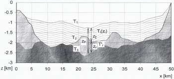
Fig. 1. Geometry of the theoretical permafrost model. For definitions of the parameters see text. Hatched lines: continental ice (the thinner lines refer to thermal isotherms). Lighter shading: permafrost and bedrock (base ≈ −2°C isoline). Darker shading: unfrozen bedrock. The values of permafrost thickness have been calculated from Equation (3). In areas where Zr ≈ 0 the temparature at the ice base is about −2°C; i.e. The ice is “warm based”. The vertical exaggeration is about 15:1.
Calculation of the temperature vs depth curve in the ice
We define the parameters (see Fig. 1) as follows. Τ 1(°C) is the temperature at the ice surface, roughly equal to the average annual temperature in the area (in this model −15°C); T 2(°C) is the temperature at the base of the ice, T i(z1); and T 3(°C) is the temperature at the base of the permafrost, roughly equal to the freezing/melting temperature of saline waters enriched below permafrost (≈ −2°C).
The ice thickness z I(km) can be interpreted from gravity or radar measurements. In Figure 1 the icethickness varies between 0 and 1.25 km.
The depth to the bottom of the permafrost, zp (km) (depth to electrically conductive saline waters enriched below permafrost), is determined by electromagnetic measurements. We thus obtain the permafrost thickness in thebedrock from zr (km) = z P – z I.
By plotting the permafrost thickness (z r) as a function of ice thickness (z I) we obtain an estimate of the temperature gradient (T r′) in the frozen bedrock from the equation:
where Z r0 ≈ z r(z 1 = 0) is the permafrost thickness beneath exposed bedrock.
The temperature at the base of the permafrost in ice-covered bedrock can be written:
We thus obtain:
which is the temperature value at the base of the ice (= T 2). In Equation (3) the temperature gradient in the bedrock (T r′) is assumed to be constant in the survey area, and the ice thickness (z I) and permafrost thickness (z r) are known for each survey point. Thus, when measuring the permafrost thickness values for variable ice-thickness values in the survey area we obtain from Equation (3) the ice-base temperature values as a function of Z I i.e. an estimate of the curve T i(z i).
It must he emphasized that the temperature vs depth curve in the ice can be estimated using the model described aboveif the temperature isotherms in the ice follow the course of the ice topography. If this assumption is valid we can construct even arbitrary higher-degree temperature vs depth curves T i(z i) for the ice using Equation (3). For example, temperature vs depth curves measured in various glaciers (e.g. Paterson, 1994) indicate that in many cases they are higher-degree curves, presumably due to a complicated combination of both conduction and advection. In such cases the interpretation of T i(z i) depends on the stability of the velocity of the ice flow and heat conduction in the survey area. The reliability of the interpreted higher-degree T i(z i) curve can be evaluated from the variation of measured (z I, z r) values along the regression curve.
It is not possible to obtain estimates of the temperature vs depth curve T i(z i) in the ice using our method if it varies throughout the survey area. However, we still can estimate permafrost thickness and temperature values at the ice base. The ice and permafrost thicknesses can be evaluated by using the geophysical methods described above. The temperature value at the ice base can then be calculated using the estimation of the temperature gradient in bedrock and permafrost thickness. If the temperature gradient in the bedrock cannot be determined from the permafrost-thickness vs ice-thickness curve it can be evaluated directly by measuring the permafrost thickness in outcrop.
Effect of electrically conductive bedrock
The method described above works best in areas where the proportion of electrically conductive rock types (e.g. graphite-bearing schists) is small, as within crystalline basement or volcanies. The effect of conductive rocks can be evaluated from the permafrost-thickness (z r) vs ice-thickness (z i) curve. If a good correlation exists between these two parameters, there is reason to believe that the couductors represent saline waters below permafrost, because a correlation between ice thickness and the depth of lithological conductors is unlikely. This is demonstrated in the following example.
Example: Measurements in Antarctica
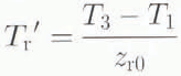
During the austral summer 1993–94 a Finnish expedition team carried out geophysical and geological investigations in western Dronning Maud Land, Antarctica. The area studied belongs to the Vestfjella mountains in Dronning Maud Land, near the Finnish base station Aboa (73°03′S, 13°25′W; black rectangle in Fig. 2a). The main aim of the geophysical measurements was to study the bedrock geology, between the nunataks.
Fig. 2. Location of the survey area (a) and the measured profiles (b).
Gravity and magnetic profiles were measured between the nunataks Basen and Plogen (≈22 km) and Basen and Fossilryggen (≈38 km) with a station spacing of 250 m (Fig. 2b). The corresponding electromagnetic profiles had station spacings varying from 250 to 1000 m. The profiles have a common starting-point on an outcrop on Basen, and the angle between the profiles is about 50–. The region is covered by ice up to about 1000 m thick; only nunataks rise abovethe ice surface. Radio-echo profiles have been measured parallel to both profiles by a Swedish expedition team (Holmlund, 1994). They also reported that the maximum velocity of the ice in lhe Basen–Plogen profile close to Plogen is about 90 myear−1. No velocity values have been reported for the Basen–Fossilryggen profile. The geology in the area has been described by Grind and others (1991); the main rock types exposed on the nunataks are basalts intruded by mafic sills. On Fossilryggen, sedimentary rocks with some graphite-bearing layers are also present. The petrophysical parameters of the rocks were defined from samples collected by geologists. The geophysical and petrophysical measurements and their use in the interpretation of bedrock geology and ice-thickness variations are described in more detail by Lehtimäki and Ruotoistenmäki (1995) and Ruotoistenmäki and Lehtimäki (1997). In this paper we concentrate only on the results concerning the evaluation of permafrost.
Electromagnetic Interpretation: Evaluation of the Thickness of the Permafrost and Temperature Variations in Ice and Bedrock
The electromagnetic sounding work was carried out with the multifrequency (2–20 000 Hz) electromagnetic sounding sytem “Sampo” described by Soininen and Jokinen (1991). The transmitter used was a horizontal loop witha diameter of 50 m, The receiver measures three components of the magnetic field. The coil separation can be increased to 1500m, in which case the depth penetration is also about 1500 m.
Along the Basen–Fossilryggen profile, in areas where the ice thickness was mainly less than 650m, soundings with a 1000 m coil separation showed significant conductors (20–500Ωm) situated within the bedrock (Figs 3 and 4). The soundings on thick ice (>650m) revealed no conductors. In the Basen–Plogen profile, conductors were detected only in the beginning of the profile where the ice thickness was less than about 650m. No conductors were observed even with greater coil separations in the main part of the profile, where the ice thickness exceeds 650 m.
Fig. 3. An example of the electromagnetic interpretation along lhe Basen–Fossilryggen profile at point x = 6000. The interpreted depths to the base af ice and permafrost have been drawn with dashed lines.
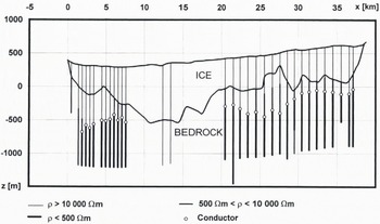
Fig. 4. Interpretation of electromagnetic soundings along the Basen–Fossilryggen profile. The white dots indicate the conductor depths used in correlation analysis in Figure 5. The variations of the ice thicknesses have been evaluated by gravity interpretation (Ruotoistenmäki and Lehtimäki, 1996) and radar measurements (Holmlund, 1994). The resistivities are represented by three broad ranges. The vertical exaggeration is 11:1.
The deep conductors observed in the bedrock have two possible explanations: (1) graphite-bearing sedimentary layers in basalts; (2) saline water layers enriched below the base of the permafrost. The latter process has been described by Daniels and others (1976), Pisarskii (1983) and Nurmi (1985). These two alternatives were evaluated by calculating the correlation between the ice thickness and the depth of the conductor in the bedrock (Fig. 5).
The study revealed a statistically significant negative correlation between the variables (number of samples = 29; correlation = 0.83; significance level at which null hypothesis of zero correlation is disproved = 0.25 × 10⁻⁷). Such a correlation could be caused by glacial erosion in bedrock above conductors which are situated at constant depth. However, from Figure 4 it can be seen that the depth variation between the conductors is about 500 m with respect to the sea-level surface (z = 0). Moreover, such a correlation due io tectonic processes is improbable.Thus, we can conclude that the conductors are not sedimentary layers but predominantly represent saline groundwaters enriched beneath the permafrost layer. The regression curve also indicates that the temperature vs depth curve is close to linear in the profile area.
The high ice velocities in the neighbouring Basen–Plogen profile suggest that in the Basen–Fossilryggen profile under consideration, the temperature variations in the ice are not defined merely by conduction, but probably also by advection. However, the results of measurements by Echelmeyer and Harrison (1994) and Engelhardt and Kamb (1994) from an ice stream in Antarctica show that even in ice streams the temperature vs depth curve can sometimes be reasonably approximated by a straight line through most of the ice column. The small variation in measured z I, z r values along the regression line in Figure 5 also suggests that the first-degree approximation is relatively good in the survey area.
From the regression line we can estimate that the ice base will be at melting point (no permafrost) for ice thicknesses greater than about 650 m (z r = 0, z I = 658 m in Fig. 5) and that the base of the permafrost in outcropping bedrock is at about 1 km (z r = 0, z I = 992 m). These results also explain why no conductors were found in the main part of the Basen–Plogen profile: because of the greaterthickness of the ice sheet the ice base was “warm” and no saline waters enriched by permafrost are present. Using the average annual surface temperature in the area of about −15°C (Taalas and others, 1991) and taking the freezing point of saline waters as −2°C, we can estimate the mean linear temperature gradients inthe ice and in the bedrock to be about 13°C/658 m≈20°Ckm−1, and 13°C/992 m≈ 13° Ckm−1, respectively.
In areas covered by thin ice or in outcrop no conductors were observed. This was because the penetration depth of theconfiguration of the electromagnetic soundings we used was too small.
It must be emphasised that we do not necessarily attribute all conductors to the effect of saline waters. For example, the conductors near Fossilryggen probably represent a mixture of graphite-bearing schists and saline waters.
Conclusions
In bedrock covered by continental ice, the depth to saline waters enriched below permafrost can be defined by electromagnetic measurements. Thus, if the ice thickness is known we can estimate permafrost-thickness variations in the surveyarea. Moreover, using the relation between the ice and permafrost thicknesses and approximations of the melting temperature of saline waters combined with the average annual surface temperature, we can estimate the temperature variations inthe bedrock and the ice. Using these estimates of temperature gradients we can also evaluate the temperature values at the base of the ice.
The results of field measurements on glaciated terrain in Antarctica support the conclusion that the method is applicable even in areas where occasional lithological conductors are to be expected. In conjunction with depth information for the ice, the electromagnetic measurements provide information concerning the distribution and conductivity of the saline water layers enriched below the permafrost. Using the average annual temperature in the survey area and the melting/freezing temperature of saline waters, we can obtain estimates of temperature variations in both the bedrock and the ice.In the future, the method should be tested in various other profiles in the survey area. In particular, we should try toobtain values for the “dashed” parts of the regression line in Figure 5. Rock samples from the lower exposures of the steep, vertically faulted cliffs should also be taken to analyze the porosity of the bedrock. Using the porosity and the electrical conductivity values we can then obtain estimates of the salinity of the groundwaters. Moreover, the method should also be tested in non-glaciated terrain where thick layers of permafrost are known to have existed since the last ice age. Also, the results of our measurements indicate that in the planning of future deep-drilling projects in areas covered by continental ice, the possibility of drilling on thinner ice and continuing the drilling in the bedrock below the base of permafrost down to the underlying conductors should also be considered. In the planning of such work, our method could be appropriate and the Basen–Fossilryggen region could be suitable for this purpose.
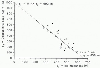
Fig. 5. Basen–Fossilryggen profile: the relation between the ice thickness and depth of the conductorin the bedrock.
Acknowledgements
We want to thank our Swedish colleagues J.-O. Näslund and P. Holmlund for providing us with radar data and P. Jansson for measuring the coordinates of the tie-points of our profiles. Moreover we wish to thank our fellow geologistsR. Blomqvist, P. Vuorela, K. Nenonen and H. Hirvas from the Geological Survey of Finland (GSF) for pointing out possibleexplanations for our observations. Finally, we express our gratitude to the GSF and the Ministry of Trade and Industry, Finland, for supporting the Finnish Antarctic Research Programme“Finnarp 93–94”.


