


Introduction
Areas of Concern (AOCs) were established in 1987 as part of the Great Lakes Water Quality Agreement (GLWQA) between the United States and Canada. AOCs are coastal locations around the Great Lakes region that have been highly degraded from human activity to a point where water-related beneficial uses are significantly impaired (EPAa). The goal of the GLWQA’s AOC program is to restore AOCs by removing beneficial use impairments (BUIs), which can range from restrictions on fish and wildlife consumption, to beach closings, to degradation of esthetics; BUIs are directly experienced by those living in the vicinity of AOCs. An AOC can be delisted once all BUIs associated with it have been removed. To accomplish this, AOCs have been the targets of extensive and expensive remediation efforts. Between 1985 and 2019, the United States and Canada spent $22.78 billion on AOC remediation efforts (Hartig et al. Reference Hartig, Krantzberg and Alsip2020). With currently 6 of the original 43 AOCs delisted, substantial restoration work remains to be done.
Economic research provides evidence that pollution damages associated with AOCs – and the potential benefits of remediation efforts – are significant. Most of this research uses property value hedonic methods and identifies damages using measures of the proximity of home sales to AOCs. Braden et al. (Reference Braden, Taylor, Won, Mays, Cangelosi and Patunru2008a) conducted a hedonic analysis of residential locations around the Buffalo River AOC and estimated aggregate benefits of cleanup to be $61 million to $118 million, depending on the size of the affected area. Braden et al. (Reference Braden, Won, Taylor, Mays, Cangelosi and Patunru2008b) used the same methodology and estimated that the aggregate benefits of cleaning up the Sheboygan River AOC would be $218 million. These are some of the highest estimates provided by the literature. McMillen (Reference McMillen2017) conducted a hedonic analysis of homes near the Grand Calumet River AOC, and estimated cleanup would increase values in aggregate by $6 million. Pairing property value hedonics with a travel cost analysis of waterfront recreation, Isely et al. (Reference Isely, Isely, Hause and Steinman2018) estimated that a $10 million investment to restore wetlands and stabilize shoreline in the Muskegon Lake AOC would generate $12 million in aggregate benefits in the housing market. Several studies have estimated the benefits of cleanup using stated preference methods and found comparable results (Braden et al. Reference Braden, Taylor, Won, Mays, Cangelosi and Patunru2008a; Braden et al. Reference Braden, Won, Taylor, Mays, Cangelosi and Patunru2008b; Phaneuf et al. (Reference Phaneuf, Taylor and Braden2012)).
While research shows the potential welfare gains from AOC restoration, there is growing evidence that policies to clean up surface water quality seldom pass a cost–benefit test, creating some contention as to whether these cleanup projects are worth the high price. Keiser et al. (Reference Keiser, Kling and Shapiro2018) evaluated 20 water quality policies and found that the median benefit–cost ratio of these policies was 0.37, although there was substantial variation in the ratio across specific projects. Some attribute these low benefit–cost ratios to the fact that many ecosystem services provided by clean water are not included in benefit estimation; for example, Downing et al. (Reference Downing, Polasky, Olmstead and Newbold2021) estimates that controlling eutrophication levels of Lake Erie could result in $3.1 billion of economic benefit through avoided climate damages and notes that these benefits are commonly not accounted for in the cost–benefit tests of water quality initiatives. If estimates of the accrued cost of AOC remediation efforts are accurate (Hartig et al. Reference Hartig, Krantzberg and Alsip2020), delisting AOCs would need to generate more than $529 million in benefit per AOC, on average, to generate a benefit–cost ratio greater than 1; this benefit amount appears to far exceed prior hedonic estimates (Braden et al. Reference Braden, Feng, Freitas and Won2010). An important caveat, of course, is that hedonic analysis only captures use values, and nonuse values can be sufficient to make up the difference between total benefits and costs (Loomis Reference Loomis2006; Kenney et al. Reference Kenney, Wilcock, Hobbs, Flores and Martínez2012). Nevertheless, hedonic-based estimates of use values can be crucial in assessing the benefits of remediation efforts, especially in the absence of estimates of nonuse values (Griffiths et al. Reference Griffiths, Klemick, Massey, Moore, Newbold, Simpson, Walsh and Wheeler2020).
This paper takes another look at the effect of AOCs on property values and attempts to shine new light on the benefits of restoration by using a comparison of sales before and after major cleanup actions to identify the effect of remediation. Our hedonic analysis focuses on the sales price of homes around the Milwaukee Estuary AOC, a portion of which experienced remediation in 2011–2015. Our contribution is twofold: first, we extend prior research that examines the effect of AOCs on nearby property values (e.g. Braden et al. Reference Braden, Taylor, Won, Mays, Cangelosi and Patunru2008a, Reference Braden, Won, Taylor, Mays, Cangelosi and Patunru2008b, and Isely et al. Reference Isely, Isely, Hause and Steinman2018) with the Milwaukee application. Second, we use the 2011–2015 remediation project to identify the effect of a discrete reduction in polychlorinated biphenyls (PCBs) and habitat restoration on sales prices by comparing prices over time and in different segments of the AOC, including segments that were not affected by remediation. In doing so, this paper aligns prior research on AOCs more closely with trends in quasi-experimental designs in the environmental and resource economics literature (e.g. Bin et al. Reference Bin, Landry and Meyer2009; Cosgrove et al. Reference Cosgrove, LaFave, Dissanayake and Donihue2015; Greenstone and Gayer Reference Greenstone and Gayer2009). This is important because most previous research on the benefits of AOC remediation was conducted before actual remediation took place and, instead, measured the damages of AOCs by comparing the prices of homes at different distances from the water. This approach can be used to estimate the benefits of cleanup, assuming remediation removes the negative proximity effect of AOCs. To our knowledge, however, this assumption remains largely untested. Moreover, prior research could have underestimated the benefits of cleanup due to problems with correlated unobservables; water quality and pollution affect prices but so do esthetics, so the proximity effect may not necessarily be negative in locations with a mix of BUIs and unimpaired beneficial uses. In contrast, Melstrom (Reference Melstrom2022) and Donnelly and Melstrom (Reference Donnelly and Melstrom2022) present ex post valuation studies of remediation in Milwaukee, but their research design uses residential sorting models rather than traditional property value hedonics as we do here. By examining sales before and after remediation, in affected and unaffected locations, our research can further substantiate earlier evidence that restoring AOCs increases local housing prices.
Background
The Milwaukee Estuary AOC includes the City of Milwaukee’s Lake Michigan shoreline and portions of the Menomonee, Kinnickinnic, and Milwaukee Rivers. A map of the estuary is shown in Figure 1. The estuary is heavily polluted due to decades of industrial wastewater dumping, municipal sewage outflow, and runoff (Milwaukee Estuary AOC, EPA). Toxic contaminants, including PCBs, heavy metals such as mercury, and petroleum byproducts, have accumulated in sediment deposits and made parts of the Milwaukee Estuary toxic to fish, wildlife, and people. Of the 14 beneficial uses that AOCs should be supporting, 10 are impaired in the Milwaukee Estuary AOC. BUIs in the estuary include beach closings, restrictions on fish and wildlife consumption, and the loss of fish and wildlife habitat.
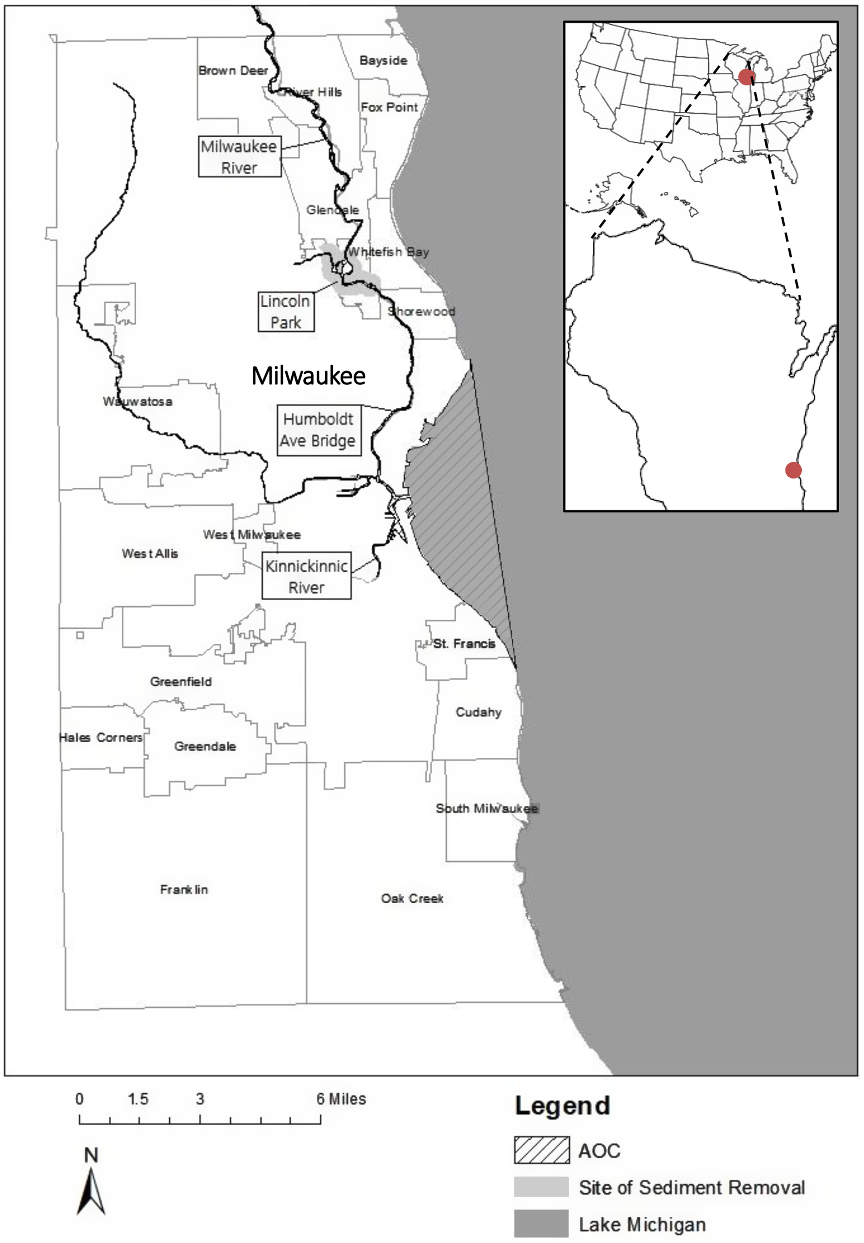
Figure 1. Milwaukee Estuary AOC in the Milwaukee metropolitan area. The AOC portion that includes the upper Milwaukee River north of the area is not shown.
Cleanup actions have taken place at several locations in the estuary. In 2008, the Wisconsin Department of Natural Resources (DNR) led cleanup of a part of the Milwaukee River near Lincoln Park, just under 9 km north of downtown Milwaukee, removing 4,000 cubic yards of contaminated sediment and 800 pounds of PCBs. In 2009, the US Environmental Protection Agency (EPA) administered the removal of 170,000 cubic yards of contaminated sediment containing 1,200 pounds of PCBs from 2,000 feet of the Kinnickinnic River. In 2011–2015, the Wisconsin DNR and U.S. EPA cleaned up an approximately 1.5km section of the Milwaukee River in two phases. Like the 2008 cleanup, this two-phase project took place near Lincoln Park. The first phase occurred between August 2011 and August 2012 and removed 140,000 cubic yards of sediment and 5,000 pounds of PCBs. The second phase occurred between October 2014 and November 2015 and removed 52,000 cubic yards of sediment and 2,300 pounds of PCBs. During the same period, following sediment removal, 12 acres of wetland and riparian habitat were restored. One of the remediation goals was to support removal of four BUIs, including restrictions on fish and wildlife consumption, degradation of fish and wildlife habitat, degradation of benthos (i.e. organisms at the bottom of the river and lake), and restrictions on dredging.
In this paper, we examine the effect of the 2011–2015 cleanup actions on home sales prices. We focus on these particular actions because they are the most recent and significant actions to date, removing “the largest known deposit of PCB-contaminated sediment in the Milwaukee River Estuary Area of Concern” (EPAb). We measure the effect of the PCB reduction by comparing the properties surrounding the remediated area to properties farther away, by applying regression analysis to a hedonic property value model and data before and after the 2011–2015 cleanup actions. Given part of this area was remediated in 2008, our estimates will reflect the additional actions that took place to more fully remove PCBs and restore habitat. Information on the economic benefit of these actions is needed for a full accounting of the effects of remediation as it is not clear that these actions consistently pass cost–benefit tests, given the high cost of remediating even small portions of AOCs (the 2011–2015 cleanup actions examined here cost $48 million (Dow Reference Dow2020)).
If buyers have environmental quality preferences, cleanup can affect home sales prices as long as they are knowledgeable about contamination and any subsequent remediation actions. There are several ways that prospective buyers in Milwaukee could have been aware of the AOC, BUIs, and the remediation actions that took place between 2011 and 2015. First, Milwaukee River fish consumption advisories due to contamination have been issued for decades (Wisconsin DNR 2013; Urban Milwaukee 2016). Second, local environmental organizations, such as Milwaukee Riverkeeper and Clean Wisconsin, are active in water monitoring, reporting on and advocating for water quality improvement actions. Third, the 2011–2015 remediation actions took place in public areas that would have been apparent to local residents and passersby. Fourth, the news media reported on cleanup efforts (e.g. Urban Milwaukee 2015), including several articles in the region’s primary newspaper, the Milwaukee Journal Sentinel (e.g. Milwaukee Journal Sentinel 2011, 2014).
One challenge in linking prices to environmental quality is whether one should use scientifically based or nontechnical measures to describe environmental quality. For the purposes of this paper, we explore the effect of quality on price using two nontechnical measures: proximity to the river and the timing of cleanup. Unfortunately, data on PCB concentrations in the water, fish, or wildlife habitat are not published systematically to estimate an effect in the Milwaukee Estuary AOC (though see Custer et al. (Reference Custer, Custer and Dummer2021) for evidence that the remediation action successfully reduced PCBs in the local environment). We also lack data on subjective perceptions of the AOC, which prior research has shown to be useful in identifying the effect of water quality on price (Poor et al. Reference Poor, Boyle, Taylor and Bouchard2001; Czajkowski and Bin Reference Czajkowski and Bin2010). We cannot therefore link price to quantitative changes in water quality (e.g. Poor et al. Reference Poor, Pessagno and Paul2007; Walsh et al. Reference Walsh, Milon and Scrogin2011). However, our nontechnical measures – proximity to water with BUIs, and the timing of remediation – align with prior hedonic research that finds water quality effects depend on proximity as well as discrete changes in ecosystem services (Mendelsohn et al. Reference Mendelsohn, Hellerstein, Huguenin, Unsworth and Brazee1992; Horsch and Lewis Reference Horsch and Lewis2009; Walsh et al. Reference Walsh, Milon and Scrogin2011; Kim et al. Reference Kim, Boxall and Adamowicz2016). Moreover, the intersection of our measures – proximity to the river after remediation – can provide insights into the perceived benefits of cleaning up PCBs and restoring fish and wildlife habitat in a major urban area (Walsh et al. Reference Walsh, Griffiths, Guignet and Klemick2017). Given the prevalence of park facilities and public trails along the Milwaukee River downstream of where remediation took place, prior research suggests that the effect on nearby sales prices should be positive (Netusil et al. Reference Netusil, Jarrad and Moeltner2019).Footnote 1
Empirical strategy
Our analysis builds off the assumption in hedonic theory that the price of a good reflects the culmination of characteristics associated with that good. We estimate three hedonic models in which the sales price of a home is a function of variables that describe structural attributes, neighborhood characteristics, and distance to landscape features (Mendelsohn and Olmstead Reference Mendelsohn and Olmstead2009). Our hypotheses are that prices are depressed near the AOC but recover in the vicinity of the Milwaukee River following the removal of PCB-contaminated sediments and habitat restoration. The first model is
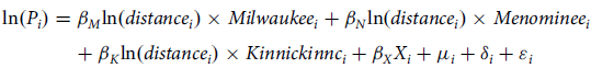 \begin{align}\ln \left( {{P_i}} \right) &= {\beta _M}{\rm{ln}}\left( {distanc{e_i}} \right) \times Milwauke{e_i} + {\beta _N}{\rm{ln}}\left( {distanc{e_i}} \right) \times Menomine{e_i}\\
&\quad + {\beta _K}{\rm{ln}}\left( {distanc{e_i}} \right) \times Kinnickinn{c_i} + {\beta _X}{X_i} + {\mu _i} + {\delta _i} + {\varepsilon _i}\end{align}
\begin{align}\ln \left( {{P_i}} \right) &= {\beta _M}{\rm{ln}}\left( {distanc{e_i}} \right) \times Milwauke{e_i} + {\beta _N}{\rm{ln}}\left( {distanc{e_i}} \right) \times Menomine{e_i}\\
&\quad + {\beta _K}{\rm{ln}}\left( {distanc{e_i}} \right) \times Kinnickinn{c_i} + {\beta _X}{X_i} + {\mu _i} + {\delta _i} + {\varepsilon _i}\end{align}
where P
i
is the price of home i, $distanc{e_i}$
measures the home’s proximity to the nearest point of the AOC,
$distanc{e_i}$
measures the home’s proximity to the nearest point of the AOC, ${X_i}$
is a vector of property structure attributes,
${X_i}$
is a vector of property structure attributes, ${\mu _i}$
is a vector of indicators for the month the sale occurred, and
${\mu _i}$
is a vector of indicators for the month the sale occurred, and ${\delta _i}$
is a vector of tract indicators to control for neighborhood characteristics. The model separates the effect of AOC proximity based on whether the nearest point lies on the Milwaukee River, Menominee River, or Kinnickinnic River, measured by the indicators
${\delta _i}$
is a vector of tract indicators to control for neighborhood characteristics. The model separates the effect of AOC proximity based on whether the nearest point lies on the Milwaukee River, Menominee River, or Kinnickinnic River, measured by the indicators $Milwauke{e_i}$
,
$Milwauke{e_i}$
, $Menomine{e_i}$
, and
$Menomine{e_i}$
, and $Kinnickinn{c_i}$
. This separation allows us to control for differences in water quality and esthetics associated with each river. The nonlinear, double-log specification of the model aligns with recommendations in the hedonic literature (Kuminoff et al. Reference Kuminoff, Parmeter and Pope2010; Bishop et al. Reference Bishop, Kuminoff, Banzhaf, Boyle, von Gravenitz, Pope, Smith and Timmins2020) and provides for an intuitive interpretation of proximity effects (Walsh et al. Reference Walsh, Milon and Scrogin2011), in which, for j = M, N, K,
$Kinnickinn{c_i}$
. This separation allows us to control for differences in water quality and esthetics associated with each river. The nonlinear, double-log specification of the model aligns with recommendations in the hedonic literature (Kuminoff et al. Reference Kuminoff, Parmeter and Pope2010; Bishop et al. Reference Bishop, Kuminoff, Banzhaf, Boyle, von Gravenitz, Pope, Smith and Timmins2020) and provides for an intuitive interpretation of proximity effects (Walsh et al. Reference Walsh, Milon and Scrogin2011), in which, for j = M, N, K, ${\beta _j}$
measures the percentage change in price for a 1% increase in distance.
${\beta _j}$
measures the percentage change in price for a 1% increase in distance.
Equation (1) is intentionally analogous to the model employed by Braden et al. (Reference Braden, Won, Taylor, Mays, Cangelosi and Patunru2008b) in their hedonic cross-section analysis estimating the property damages of the Sheboygan River AOC. Their model used logged distance, plus logged distance interacted with indicators for the lower and middle segments of the Sheboygan River, to estimate the effect of living near different parts of the AOC on housing values. Braden et al. (Reference Braden, Won, Taylor, Mays, Cangelosi and Patunru2008b) found properties farther from the AOC tended to have higher prices, with a stronger effect near the upper river than the lower river. Braden et al. (Reference Braden, Won, Taylor, Mays, Cangelosi and Patunru2008b) then used the negative proximity effect to measure the capital losses associated with the AOC, which they found were concentrated in the upper river. By estimating equation (1) using sales data from before the 2011–2015 remediation actions, we can use the same research design to estimate the capital losses from the Milwaukee Estuary AOC and determine whether these losses tend to be concentrated in the Milwaukee River, Menominee River, or Kinnickinnic River.Footnote 2
A potential complication of the above research design is that proximity to the AOC could be correlated with unobserved amenities, that is, a correlated unobservables problem. For example, cities develop in stages, so there may be certain types of houses that are more likely to be in close proximity to the AOC. Furthermore, distance to the AOC is essentially equivalent to distance to the water, which will include beneficial uses in addition to the BUIs in the Milwaukee Estuary; for properties near the water, the amenity effect could overwhelm the AOC effect. If these correlations are present in the Milwaukee Estuary AOC, then ${\beta _j}$
for j = M, N, K will not measure the effect of AOC proximity alone. To the extent that home types and/or access to beneficial uses is largely neighborhood-specific, the tract fixed effects included in equation (1) could take care of this problem, as appears to have been the case in prior research (e.g. Braden et al. (Reference Braden, Taylor, Won, Mays, Cangelosi and Patunru2008a)). However, with access to home sales over many years, we do not have to rely on distance alone. Rather, we can leverage the 2011–2015 remediation actions as a natural experiment to identify the effect of a discrete reduction in PCB concentrations and additional wildlife habitat.
${\beta _j}$
for j = M, N, K will not measure the effect of AOC proximity alone. To the extent that home types and/or access to beneficial uses is largely neighborhood-specific, the tract fixed effects included in equation (1) could take care of this problem, as appears to have been the case in prior research (e.g. Braden et al. (Reference Braden, Taylor, Won, Mays, Cangelosi and Patunru2008a)). However, with access to home sales over many years, we do not have to rely on distance alone. Rather, we can leverage the 2011–2015 remediation actions as a natural experiment to identify the effect of a discrete reduction in PCB concentrations and additional wildlife habitat.
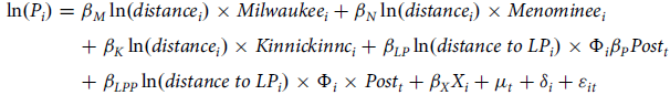
The second model incorporates a panel data design:
 \begin{align}\ln \left( {{P_i}} \right) &= {\beta _M}\ln \left( {distanc{e_i}} \right) \times Milwauke{e_i} + {\beta _N}\ln \left( {distanc{e_i}} \right) \times Menomine{e_i}\\
&\quad + {\beta _K}\ln \left( {distanc{e_i}} \right) \times Kinnickinn{c_i} + {\beta _{LP}}\ln \left( {distance\;to\;L{P_i}} \right) \times {\Phi _i}{\beta _P}Pos{t_t}\\
&\quad + {\beta _{LPP}}\ln \left( {distance\;to\;L{P_i}} \right) \times {\Phi _i} \times Pos{t_t} + {\beta _X}{X_i} + {\mu _t} + {\delta _i} + {\varepsilon _{it}}\end{align}
\begin{align}\ln \left( {{P_i}} \right) &= {\beta _M}\ln \left( {distanc{e_i}} \right) \times Milwauke{e_i} + {\beta _N}\ln \left( {distanc{e_i}} \right) \times Menomine{e_i}\\
&\quad + {\beta _K}\ln \left( {distanc{e_i}} \right) \times Kinnickinn{c_i} + {\beta _{LP}}\ln \left( {distance\;to\;L{P_i}} \right) \times {\Phi _i}{\beta _P}Pos{t_t}\\
&\quad + {\beta _{LPP}}\ln \left( {distance\;to\;L{P_i}} \right) \times {\Phi _i} \times Pos{t_t} + {\beta _X}{X_i} + {\mu _t} + {\delta _i} + {\varepsilon _{it}}\end{align}
The specification is similar to equation (1), except for three new terms: the first measures the effect of proximity to where remediation occurred, where $distance\;to\;L{P_i}$
is the natural log of the distance between each property and the center of the Lincoln Park remediation site and
$distance\;to\;L{P_i}$
is the natural log of the distance between each property and the center of the Lincoln Park remediation site and ${{\rm{\Phi }}_i}$
is an indicator that takes the value one if this distance is less than 5 km. The indicator truncates the proximity effect so that homes more than 5 km away have no influence on the estimates, because the effect of the park on the demand for homes is likely to be highly localized. The second new term,
${{\rm{\Phi }}_i}$
is an indicator that takes the value one if this distance is less than 5 km. The indicator truncates the proximity effect so that homes more than 5 km away have no influence on the estimates, because the effect of the park on the demand for homes is likely to be highly localized. The second new term, $Pos{t_t}$
, is an indicator that equals 1 if the home was sold in the postproject period and 0 if the sale occurred in the preproject period. The third new term,
$Pos{t_t}$
, is an indicator that equals 1 if the home was sold in the postproject period and 0 if the sale occurred in the preproject period. The third new term, $distance\;to\;L{P_i} \times {{\rm{\Phi }}_i} \times Pos{t_t}$
, accounts for the change in the proximity effect after remediation. This model assumes that homes sold in the vicinity of Lincoln Park in the postproject period are impacted by remediation, with the impact scaling proportionately with distance. If households value water quality improvements, then the coefficient on the interaction term will be negative, because living near Lincoln Park becomes more desirable (i.e. living farther away becomes less desirable) after remediation.
$distance\;to\;L{P_i} \times {{\rm{\Phi }}_i} \times Pos{t_t}$
, accounts for the change in the proximity effect after remediation. This model assumes that homes sold in the vicinity of Lincoln Park in the postproject period are impacted by remediation, with the impact scaling proportionately with distance. If households value water quality improvements, then the coefficient on the interaction term will be negative, because living near Lincoln Park becomes more desirable (i.e. living farther away becomes less desirable) after remediation.
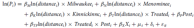
The third model assumes the effect on prices extends down the part of the AOC that experienced reductions in PCB concentrations after remediation, rather than at Lincoln Park per se:
 \begin{align}\ln \left( {{P_i}} \right) &= {\beta _M}{\rm{ln}}\left( {distanc{e_i}} \right) \times Milwauke{e_i} + {\beta _N}{\rm{ln}}\left( {distanc{e_i}} \right) \times Menomine{e_i}\\
&\quad + {\beta _K}{\rm{ln}}\left( {distanc{e_i}} \right) \times Kinnickinn{c_i} + {\beta _T}{\rm{ln}}\left( {distanc{e_i}} \right) \times Treate{d_i} + {\beta _P}Pos{t_t}\\
&\quad + {\beta _{TP}}{\rm{ln}}\left( {distanc{e_i}} \right) \times Treate{d_i} \times Pos{t_t} + {\beta _X}{X_i} + {\mu _t} + {\delta _i} + {\varepsilon _{it}}\end{align}
\begin{align}\ln \left( {{P_i}} \right) &= {\beta _M}{\rm{ln}}\left( {distanc{e_i}} \right) \times Milwauke{e_i} + {\beta _N}{\rm{ln}}\left( {distanc{e_i}} \right) \times Menomine{e_i}\\
&\quad + {\beta _K}{\rm{ln}}\left( {distanc{e_i}} \right) \times Kinnickinn{c_i} + {\beta _T}{\rm{ln}}\left( {distanc{e_i}} \right) \times Treate{d_i} + {\beta _P}Pos{t_t}\\
&\quad + {\beta _{TP}}{\rm{ln}}\left( {distanc{e_i}} \right) \times Treate{d_i} \times Pos{t_t} + {\beta _X}{X_i} + {\mu _t} + {\delta _i} + {\varepsilon _{it}}\end{align}
The new term, ${\rm{ln}}\left( {distanc{e_i}} \right) \times Treate{d_i}$
, interacts proximity to the AOC with
${\rm{ln}}\left( {distanc{e_i}} \right) \times Treate{d_i}$
, interacts proximity to the AOC with $Treate{d_i}$
, which equals 1 for homes whose nearest point on the AOC is in the affected area and 0 otherwise. The affected area includes the Milwaukee River running from Lincoln Park to the Humboldt Avenue Bridge, which separates the upper estuary from the lower estuary (Figure 1). This segment runs 8 km downstream from the center of sediment remediation. Using this approach, the treated group includes homes whose closest point on the AOC lies between Lincoln Park and the Humboldt Avenue Bridge. The coefficient
$Treate{d_i}$
, which equals 1 for homes whose nearest point on the AOC is in the affected area and 0 otherwise. The affected area includes the Milwaukee River running from Lincoln Park to the Humboldt Avenue Bridge, which separates the upper estuary from the lower estuary (Figure 1). This segment runs 8 km downstream from the center of sediment remediation. Using this approach, the treated group includes homes whose closest point on the AOC lies between Lincoln Park and the Humboldt Avenue Bridge. The coefficient ${\beta _T}$
measures the proximity effect among homes in the treated group. The interaction
${\beta _T}$
measures the proximity effect among homes in the treated group. The interaction ${\rm{ln}}\left( {distanc{e_i}} \right) \times Treate{d_i} \times Pos{t_t}$
captures any change in this group after remediation, and the coefficient
${\rm{ln}}\left( {distanc{e_i}} \right) \times Treate{d_i} \times Pos{t_t}$
captures any change in this group after remediation, and the coefficient ${\beta _{TP}}$
measures the change in the proximity effect near the affected area. We expect this coefficient to be negative, which would indicate that living closer to the area where environmental quality improved became more desirable after remediation.
${\beta _{TP}}$
measures the change in the proximity effect near the affected area. We expect this coefficient to be negative, which would indicate that living closer to the area where environmental quality improved became more desirable after remediation.
We divide the study period in three to account for changes in the AOC over time (Jarrad et al. Reference Jarrad, Netusil, Moeltner, Morzillo and Yeakley2018). The first or preproject period includes the baseline conditions of the AOC. This period includes sales between August 2010 and July 2011, which is the year before the start of the project in August 2011. The second period, the project period, includes sales between the start and end of the project. The third or postproject period includes sales between December 2015 and November 2016, which is 1 year after the end of the project. Perceptions of remediation during the project phase could be dominated by traffic, construction, and excavation associated with removing contaminated sediments, which could affect sales price, so to provide for a clean pre-post comparison, we focus on sales in the first and third phases only. Assuming that property values in the treated and untreated areas were changing identically prior to remediation, panel data analysis of sales in these years can provide a valid method for estimating the effect on price.Footnote 3 Remediation can capitalize into property values at different periods, so we also consider as a robustness check the estimates when we revise the postproject period to include sales between August 2017 and July 2018, or 6 years after the start of the project (Jarrad et al. Reference Jarrad, Netusil, Moeltner, Morzillo and Yeakley2018).
Data
Due to the timing of the remediation project, arms-length sales records between 2008 and 2018 were acquired from the City of Milwaukee. These data include 1,634 sales in the preproject period, and 4,435 in the postproject period. Each sales record includes the street address, sales price and date, lot size, square feet, number of bedrooms, number of full and half bathrooms, and descriptions of the facade. We removed sales with missing values, sales of commercial and manufacturing properties, and vacant lots. We included condominiums but excluded sales of apartment buildings. Properties that had a finished square footage less than 350 and more than 10,000 were dropped. We also removed properties that sold for less than $5,000 or more than $1,000,000. We excluded all sales more than 5 km from the AOC, as prior research indicates small bodies of water are unlikely to have an effect on homes more than a few kilometers away (Braden et al. Reference Braden, Won, Taylor, Mays, Cangelosi and Patunru2008b; Walsh et al. Reference Walsh, Milon and Scrogin2011). This resulted in 3,925 sales; 1,033 in the preproject period and 2,892 in the postproject period.
Summary statistics of the home characteristics and location features can be found in Table 1. In addition to structural attributes, we also generated a set of indicators for whether a home was classified as a colonial, Cape Cod, ranch, or condominium, to control for the influence of esthetics and build quality as well as whether the home was part of a larger building complex. Following Braden et al. (Reference Braden, Taylor, Won, Mays, Cangelosi and Patunru2008a; Reference Braden, Won, Taylor, Mays, Cangelosi and Patunru2008b), in the model we enter lot size and age as second-degree polynomials to allow for nonlinear relationships between these variables and price.
Table 1. Summary statistics of Milwaukee home sales in the pre- and postproject phases
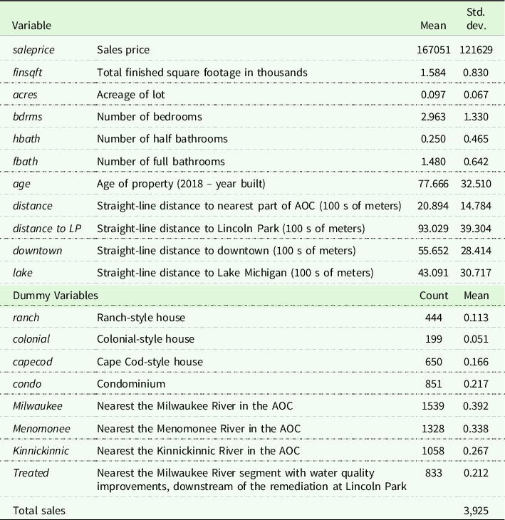
We then measured distances to several AOC and non-AOC features (Geoghegan et al. Reference Geoghegan, Lynch and Bucholtz2003; Braden et al. Reference Braden, Taylor, Won, Mays, Cangelosi and Patunru2008a). To do this, we transferred the sales to a geocoding tool to calculate the latitude and longitude of each address. We measured the shortest distance from these coordinates to the nearest point on the AOC, running from the mouth of the Milwaukee River at Lake Michigan up the Milwaukee, Menominee, and Kinnickinnic Rivers to the edge of Milwaukee’s city limits or the edge of the AOC, whichever occurred first. We then measured the distance in hundreds of meters (km/10) from each address to downtown, the lakeshore, and Lincoln Park. Table 1 presents the means of the four distance variables, which enter the model in log form. In addition, we included an indicator for homes within 150 m of the water, to account for any systematic differences between waterfront and non-waterfront homes. Finally, we used the geocoded addresses and the census tract shapefile for the City of Milwaukee to determine the tract associated with each property. Homes sales occurred in 213 tracts.
Results and discussion
Table 2 presents the main coefficients of interest in the three models. For a complete set of coefficient estimates, see the Appendix. These coefficients measure the percent change in sales price associated with a 1% increase in distance (a decrease in proximity) to the AOC, depending on whether a home is closest to the Milwaukee, Menominee, or Kinnickinnic Rivers, or the treated area. For the sake of brevity, we will not describe the other coefficients in the model (i.e. on the structural attributes and lake and downtown distance variables), except to note that the estimates are in-line with expectations and consistent with prior research. Model (1) provides no evidence that proximity affects price. In fact, the coefficients on l ${\rm{n}}\left( {distance} \right) \times Menominee$
and
${\rm{n}}\left( {distance} \right) \times Menominee$
and $\ln \left( {distance} \right) \times Kinnickinnic$
are negative, which runs contrary to expectations, though neither is statistically significant. The coefficient on
$\ln \left( {distance} \right) \times Kinnickinnic$
are negative, which runs contrary to expectations, though neither is statistically significant. The coefficient on $\ln \left( {distance} \right) \times Milwaukee$
is also not significantly different from zero.
$\ln \left( {distance} \right) \times Milwaukee$
is also not significantly different from zero.
Table 2. Hedonic models – coefficients of interest
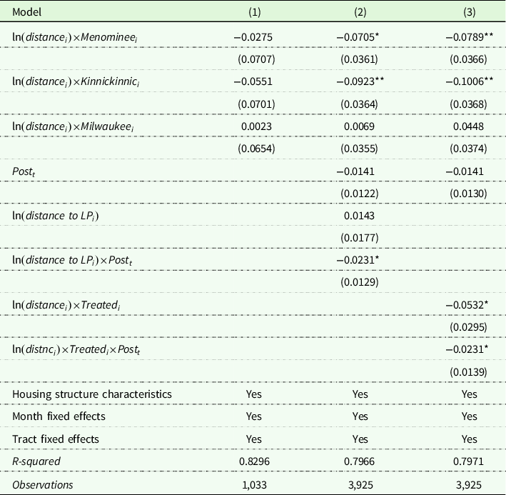
Standard errors in parentheses below coefficients. * and ** indicate significance at 10% and 5% levels, respectively.
Now consider the coefficients in model (2), which are estimated using both the pre- and postproject data. The coefficients on $\ln \left( {distance} \right) \times Menominee$
and
$\ln \left( {distance} \right) \times Menominee$
and $\ln \left( {distne} \right) \times Kinnickinnic$
are significantly negative, which implies that homebuyers place a premium on living near the Menominee and Kinnickinnic Rivers. The coefficients on
$\ln \left( {distne} \right) \times Kinnickinnic$
are significantly negative, which implies that homebuyers place a premium on living near the Menominee and Kinnickinnic Rivers. The coefficients on $\ln \left( {distance} \right) \times Milwaukee$
and
$\ln \left( {distance} \right) \times Milwaukee$
and $\ln \left( {distance\;to\;LP} \right)$
distances are both statistically insignificant. However, the coefficient on
$\ln \left( {distance\;to\;LP} \right)$
distances are both statistically insignificant. However, the coefficient on $\ln \left( {distance\;to\;LP} \right) \times Post$
is significantly negative. This indicates that a proximity premium for homes near Lincoln Park developed after remediation.
$\ln \left( {distance\;to\;LP} \right) \times Post$
is significantly negative. This indicates that a proximity premium for homes near Lincoln Park developed after remediation.
Finally, consider the coefficients of model (3), which are also estimated using the pre- and postproject data. The coefficients on $\ln \left( {distance} \right) \times Menominee$
and
$\ln \left( {distance} \right) \times Menominee$
and $\ln \left( {distance} \right) \times Kinnickinnic$
are significantly negative, similar to model (2). The coefficient on
$\ln \left( {distance} \right) \times Kinnickinnic$
are significantly negative, similar to model (2). The coefficient on $\ln \left( {distance} \right) \times Milwaukee$
is not significantly different from zero. However, the coefficient on
$\ln \left( {distance} \right) \times Milwaukee$
is not significantly different from zero. However, the coefficient on $\ln \left( {distance} \right) \times Treated$
is significantly negative, which indicates a price premium for homes in the treated area relative to those in proximity to other parts of the Milwaukee River. Turning to the effect of remediation in the treated area, the coefficient on
$\ln \left( {distance} \right) \times Treated$
is significantly negative, which indicates a price premium for homes in the treated area relative to those in proximity to other parts of the Milwaukee River. Turning to the effect of remediation in the treated area, the coefficient on $\ln \left( {distance} \right) \times Treated \times Post$
is significantly negative. To be specific, the coefficients on
$\ln \left( {distance} \right) \times Treated \times Post$
is significantly negative. To be specific, the coefficients on $\ln \left( {distance} \right) \times Treated$
and
$\ln \left( {distance} \right) \times Treated$
and $\ln \left( {distance} \right) \times Treated \times Post$
imply that before remediation a 100% increase in distance (e.g. 0.5 km to 1 km) from the AOC (in the treated area) was associated with a 5.3% reduction in price, which is $8,880 at the average price, and that after remediation the same change was associated with a 7.6% reduction, which is $12,740 using the average sale price for properties in our analysis (Table 1).
$\ln \left( {distance} \right) \times Treated \times Post$
imply that before remediation a 100% increase in distance (e.g. 0.5 km to 1 km) from the AOC (in the treated area) was associated with a 5.3% reduction in price, which is $8,880 at the average price, and that after remediation the same change was associated with a 7.6% reduction, which is $12,740 using the average sale price for properties in our analysis (Table 1).
Robustness checks
We performed three robustness checks to test the sensitivity of the estimates to the definition of the treated area, controlling for time-varying unobservables, and the timing of capitalization effects. These results are shown in Table 3. The first robustness check revises the definition of the treated area in model (3) by reducing the area from 8 to 5 km downstream of Lincoln Park. These results are shown in the first column of Table 3. This results in a more precisely estimated, larger (in absolute value) treatment effect than in Table 2. This should increase confidence that remediation affected sales prices, particularly for homes just downstream of Lincoln Park. The second column returns to the original definition of the treated area and adds tract-by-post fixed effects to correct for the influence of time-varying neighborhood characteristics that could potentially be correlated with the timing and location of remediation (e.g. major capital improvements or changes in land use). The addition of these fixed effects increases the coefficient on $\ln \left( {distance} \right) \times Treated \times Post$
; however, the estimate is less precise and no longer significantly different from zero at conventional levels. Finally, the last robustness check uses an alternative pre-post comparison, by replacing the 2,892 postproject sales with 3,404 “mature-project” sales that occurred between August 2017 and July 2018, in case the effect of cleanup takes longer to capitalize than a single year after the project ends. With tract-by-post fixed effects, the coefficient on
$\ln \left( {distance} \right) \times Treated \times Post$
; however, the estimate is less precise and no longer significantly different from zero at conventional levels. Finally, the last robustness check uses an alternative pre-post comparison, by replacing the 2,892 postproject sales with 3,404 “mature-project” sales that occurred between August 2017 and July 2018, in case the effect of cleanup takes longer to capitalize than a single year after the project ends. With tract-by-post fixed effects, the coefficient on $\ln \left( {distance} \right) \times Treated \times Post$
is significantly negative and substantially larger relative to the earlier estimates. This suggests the effect of remediation could take several years after a project end to fully materialize.Footnote
4
$\ln \left( {distance} \right) \times Treated \times Post$
is significantly negative and substantially larger relative to the earlier estimates. This suggests the effect of remediation could take several years after a project end to fully materialize.Footnote
4
Table 3. Robustness checks applied to model (3)
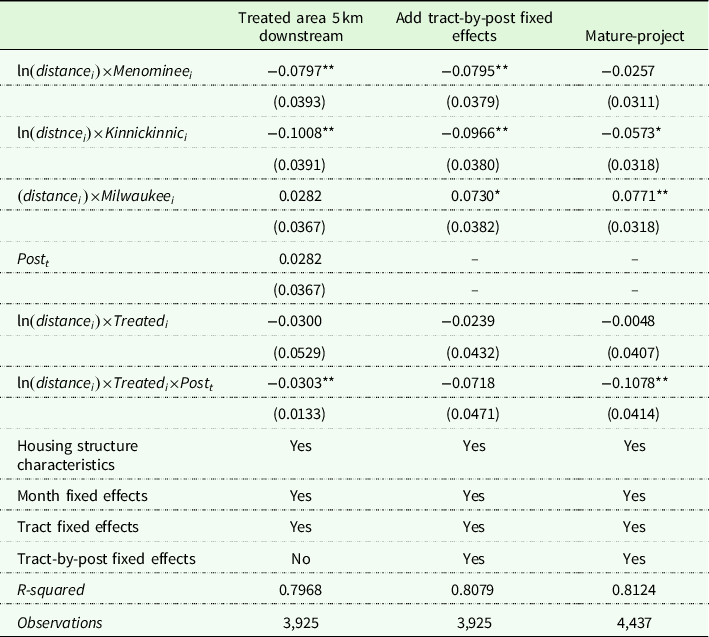
Note that the effect of Post t is not identified when the regression includes tract-by-post effects.
Standard errors in parentheses below coefficients. * and ** indicate significance at 10% and 5% levels, respectively.
Additional discussion
The results indicate that hedonic analysis based on distance cannot always estimate the effect of an AOC on home prices. The coefficients on the proximity variables in model (1) provide no evidence that homebuyers either discount or place a premium on a home’s proximity to the Milwaukee Estuary AOC. The variation in sign between different rivers in the AOC adds further uncertainty as to the actual proximity effect. Prior research has found that home values tend to rise with distance (Braden et al. Reference Braden, Taylor, Won, Mays, Cangelosi and Patunru2008a, Braden et al. Reference Braden, Won, Taylor, Mays, Cangelosi and Patunru2008b), a result which we are unable to replicate. This does not mean that buyers are indifferent to the presence of AOCs. Rather, our results suggest that, at least in some housing markets, the proximity effect of an AOC can be tempered or entirely offset by amenities near the water, as appears to be the case in Milwaukee.
The overall effects of proximity notwithstanding, the results imply that buyers care about the presence of PCBs and remediation because cleaning up part of the Milwaukee Estuary led to capital gains that increased with proximity. Both the coefficient on distance to remediation at Lincoln Park in model (2) and the coefficient on distance to the downriver segment in model (3) were significantly negative, implying that living closer to these areas became more valuable after remediation. We can use the change in the price gradient associated with the cleanup effect to estimate the capital gain from remediation, using the formula ![]() , where
, where ![]() is the hypothetical boundary distance of the effect. Given we trimmed the data to sales within 5 km, and measured distance in hundreds of meters,
is the hypothetical boundary distance of the effect. Given we trimmed the data to sales within 5 km, and measured distance in hundreds of meters, ![]() = 50. Using the coefficients in model (3) (the estimates are similar using model (2)), for a property in the treated area adjacent to the water, which we define as within 150 m, the implied capital gain is 8%, or $13,538 using the average property sales price. For properties affected by the improvement but located 3 km away, the implied capital gain is just 1%, or $1,972. Across all homes in the treated area, the implied capital gain is 3%, or $5,683. Note that the gain is larger if we were to use the coefficients in the robustness checks. For example, the implied capital gain when based on the mature-sample results is 17%, or $28,936. The market therefore appears to have put a premium on living in the treated area after remediation. This does not mean that pollution and BUIs are no longer a problem, but it does show that buyers were affected by a discrete change in PCBs as a function of their proximity to the remediation area.
= 50. Using the coefficients in model (3) (the estimates are similar using model (2)), for a property in the treated area adjacent to the water, which we define as within 150 m, the implied capital gain is 8%, or $13,538 using the average property sales price. For properties affected by the improvement but located 3 km away, the implied capital gain is just 1%, or $1,972. Across all homes in the treated area, the implied capital gain is 3%, or $5,683. Note that the gain is larger if we were to use the coefficients in the robustness checks. For example, the implied capital gain when based on the mature-sample results is 17%, or $28,936. The market therefore appears to have put a premium on living in the treated area after remediation. This does not mean that pollution and BUIs are no longer a problem, but it does show that buyers were affected by a discrete change in PCBs as a function of their proximity to the remediation area.
We can use the estimates above to calculate the total capital gain from the 2011–2015 remediation project. Given an average gain of $5,683 per house and 46,000 households in the affected area, the implied total capital gain is $261 million. This is substantially larger than the $48 million cost of the project.
An important caveat is that the effect of remediation is not precisely estimated in all models. The 90% confidence interval for the capital gain to a property at the average distance from the water is 0% to 5%, while for a property immediately adjacent to the water it is 0% to 17%, based on model (3) (similar confidence intervals are implied using model (2)). Furthermore, the robustness checks show that the coefficient of interest, level of precision, and statistical significance is sensitive to model specification. This may lead some readers to doubt whether remediation had any effect on buyer decisions. The large amount of uncertainty about the effect size, though, does not necessarily imply that the effect is zero. Our results do, however, leave open the possibility that the average effect could be as small as 1% or 2%, but also as large as 15% for properties adjacent to the water. This range appears to be slightly lower than what has been implied by prior research.Footnote 5 Of course, the remediation event studied here reduced PCB concentrations and restored habitat in only one part and did not restore the entire AOC, so the effect of complete restoration on Milwaukee properties could be much larger and, thus, in the range of prior estimates.
Conclusion
This study used hedonic analysis to estimate the effect of remediating a portion of the Milwaukee Estuary AOC on home prices. Our results did not provide evidence that the Milwaukee housing market discounts proximity to the AOC, in general. Using data on home sales prior to cleanup, the association between price and distance to various parts of the AOC were statistically insignificant. To be clear, this does not mean that households overlook water quality in their residential location decisions, because water in AOCs can provide a mix of amenities and disamenities, which is difficult to untangle using a hedonic model based on distances and cross-section data. However, when we applied hedonic analysis to sales data from before and after a major remediation project in the upper Milwaukee River, we found a significant relationship between price and distance to the cleanup area after remediation actions lowered PCB concentrations. This provides evidence that households do consider proximity to AOC-associated pollutants in location decisions.
Our results are promising for the future of remediation efforts as they indicate that discrete reductions in PCBs create value for the surrounding community. Contaminated sediment and toxic substances continue to be a problem in the Great Lakes, particularly near major cities, which reduces the value of living near the coast. While prior research on AOCs has estimated the damages of this contamination, the effect of remediating these areas has received comparatively less attention. Our research shows that prices near the water do indeed increase after cleanup. An important caveat is that the effects examined here are concentrated in the upper Milwaukee River, and that restoration of the broader Milwaukee Estuary AOC remains incomplete. Fully restoring the AOC would not only affect a larger area but could also further influence perceptions of water quality in the upper Milwaukee River. Additional research is necessary to confirm the value of fully restoring AOCs using ex post sales data.
Data availability statement
Data and code available from the corresponding author upon request.
Funding statement
Wilkinson and Melstrom received no specific grant from any funding agency, commercial, or not-for-profit sectors for this research.
Competing interests
Wilkinson and Melstrom declare none.
Appendix
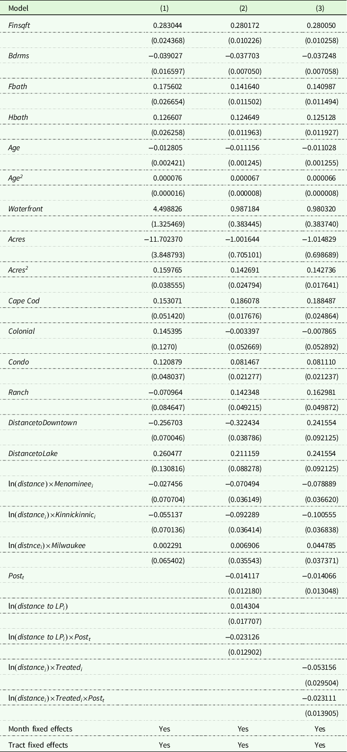
Table A1. Hedonic models – all coefficients


 Open access