


1. Introduction
Multiphase flow in porous media is of broad scientific interest reflected in an abundant literature dedicated to the subject over the past century. The description of two-phase immiscible flow in porous materials, triggered by the booming of oil recovery, was proposed nearly a century ago in the seminal work of Wyckoff & Botset (Reference Wyckoff and Botset1936) and Muskat & Meres (Reference Muskat and Meres1936), who suggested the use of a generalized Darcy's law. This long-lasting domain of interest has been enriched by many others, ranging from flow in packed bed reactors, remediation of dense non-aqueous phase liquids in contaminated soils, CO $_2$ sequestration, hydrology, wastes storage in landfills or subsurface formations, flow in biological tissues, drying of porous materials, gas–water management in fuel cells, flow in filters and membranes, among others. Various aspects of this challenging topic have been analysed by means of many different experimental, numerical and theoretical approaches at different scales of analysis, ranging from the pore scale to macroscopic scales that may include heterogeneities. A recent and comprehensive reference on the subject of multiphase flow in porous media that encompasses both pore scale and macroscale perspectives is the monograph by Blunt (Reference Blunt2017). Despite the fact that the generalized Darcy's law originally proposed by Muskat & Meres lacks physical justification, it is still of common practical use in large-scale simulators, for instance.
Experimental works at the pore scale have been carried out in systems mimicking a porous structure (Avraam & Payatakes Reference Avraam and Payatakes1995) and the recent progress in imaging techniques now provides the means to perform observations in real structures at micron to submicron scales (Singh et al. Reference Singh, Menke, Andrew, Rau, Bijeljic and Blunt2018; Hunter & Dewanckele Reference Hunter and Dewanckele2021). These observations give insightful information about the physical mechanisms at play that help in understanding macroscopic behaviours. In conjunction, two-phase flow simulations at the pore scale have also been carried out extensively (Zhao et al. Reference Zhao2019) with the aim of reproducing both microscopic and macroscopic observations. These have been performed using various representations of porous structures like pore networks (Gjennestad, Winkler & Hansen Reference Gjennestad, Winkler and Hansen2020; Maalal et al. Reference Maalal, Prat, Peinador and Lasseux2021), X-ray or scanning-electron-microscopy-based images (Aljasmi & Sahimi Reference Aljasmi and Sahimi2021; Shams et al. Reference Shams, Singh, Bijeljic and Blunt2021). Computations have been carried out in many different configurations using lattice-Boltzmann (Taghilou & Rahimian Reference Taghilou and Rahimian2014; Shi & Tang Reference Shi and Tang2018; Gu, Liu & Wu Reference Gu, Liu and Wu2021) and other techniques, either based on two-fluid systems taking explicitly into account the interfaces with a volume of fluid method (Yang et al. Reference Yang, Cai, Yao, Zhong, Zhang, Song, Zhang, Sun and Lisitsa2021) or continuous two-fluid approaches using level-set (Ambekar, Mondal & Buwa Reference Ambekar, Mondal and Buwa2021; Jettestuen, Friis & Helland Reference Jettestuen, Friis and Helland2021) or Cahn–Hilliard models (Yang & Kim Reference Yang and Kim2021) with improved algorithms making use of machine learning (see, for instance, Silva et al. (Reference Silva, Salinas, Jackson and Pain2021)).
Although pore-scale investigations are important, they remain insufficient for large-scale modelling, and macroscopic models are of major interest. To this end, several works based on upscaling techniques (Battiato et al. Reference Battiato, Ferrero, O'Malley, Miller, Takhar, Valdés-Parada and Wood2019) have been reported using the volume averaging method (Whitaker Reference Whitaker1986; Quintard & Whitaker Reference Quintard and Whitaker1988, Reference Quintard and Whitaker1990; Whitaker Reference Whitaker1994; Lasseux, Quintard & Whitaker Reference Lasseux, Quintard and Whitaker1996; Quintard & Whitaker Reference Quintard and Whitaker1999; Lasseux, Ahmadi & Arani Reference Lasseux, Ahmadi and Arani2008; Luévano-Rivas & Valdés-Parada Reference Luévano-Rivas and Valdés-Parada2015; Davit & Quintard Reference Davit and Quintard2018; Chen, Sun & Wang Reference Chen, Sun and Wang2019) and the homogenization technique (Auriault Reference Auriault1987; Auriault, Lebaigue & Bonnet Reference Auriault, Lebaigue and Bonnet1989; Bourgeat Reference Bourgeat1997; Daly & Roose Reference Daly and Roose2015; Picchi & Battiato Reference Picchi and Battiato2018), both sharing many points in common (Davit et al. Reference Davit2013). The thermodynamically constrained averaging theory (known as TCAT) was also employed to obtain averaged models (Jackson, Miller & Gray Reference Jackson, Miller and Gray2009; Gray & Miller Reference Gray and Miller2011, Reference Gray and Miller2014; Gray et al. Reference Gray, Dye, McClure, Pyrak-Nolte and Miller2015; Rybak, Gray & Miller Reference Rybak, Gray and Miller2015; McClure et al. Reference McClure, Berrill, Gray and Miller2016a,Reference McClure, Berrill, Gray and Millerb) as well as the hybrid mixture theory (Schreyer & Hilliard Reference Schreyer and Hilliard2021), among others.
In the context of volume averaging, Whitaker (Reference Whitaker1986) derived a macroscopic model for immiscible, steady and Newtonian two-phase flow in rigid and homogeneous porous media under creeping flow conditions. The model consisted of a set of two macroscopic equations for mass and momentum transport. This model was later revisited by Lasseux et al. (Reference Lasseux, Quintard and Whitaker1996) in order to express the macroscopic momentum balance equations in the form of Darcy's laws with two macroscopic pressure gradients contributions, which is consistent with the model derived by Auriault (Reference Auriault1987) using the homogenization method. The same type of model was later derived by Picchi & Battiato (Reference Picchi and Battiato2018) also using homogenization. All these macroscopic models were written in terms of four permeability tensors that can be predicted from the solution of two associated closure problems. This approach was later extended by Lasseux et al. (Reference Lasseux, Ahmadi and Arani2008) to incorporate inertial effects. However, in the analysis reported in these works, the contributions from surface tension and curvature of the fluid–fluid interface is not present at the closure level. In the context of volume averaging, such a simplification was thought as a valid one under the constraint of Bond and capillary numbers much smaller than unity (as well as of a vanishingly small Weber number value in the presence of inertia) (Whitaker Reference Whitaker1994; Lasseux et al. Reference Lasseux, Ahmadi and Arani2008). Within the framework of homogenization, this term was dropped as it was thought to be insensitive at the order of the two-scale asymptotic expansion carried out in the method. Nevertheless, these assumptions have not yet been carefully investigated, although many works have suggested that the impact of the interfacial area may be of importance, without, however, providing a closed expression of its contribution (Hassanizadeh & Gray Reference Hassanizadeh and Gray1993; Hilfer Reference Hilfer1998; Hilfer & Besserer Reference Hilfer and Besserer2000; Li, Pan & Miller Reference Li, Pan and Miller2005; Niessner & Hassanizadeh Reference Niessner and Hassanizadeh2008; Niessner, Berg & Hassanizadeh Reference Niessner, Berg and Hassanizadeh2011). An accurate and physically sound macroscopic model that does not rely on the above mentioned assumptions is still lacking, the derivation of which is the purpose of the present work.
Recently, Daly & Roose (Reference Daly and Roose2015) and Chen et al. (Reference Chen, Sun and Wang2019) used the homogenization technique and volume averaging method, respectively, to derive a macroscopic model for two-phase flow in homogeneous porous media departing from a single equation for mass balance in both phases and also for momentum transport at the microscale, together with the Cahn–Hilliard equations. This approach makes use of a phase field to distinguish the two fluid phases without assuming the existence of a sharp interface separating the two. The resulting model consists of a modification to the mass equations that includes a diffusion term of the macroscopic chemical potential in each phase. Although this approach provides an interesting alternative, the present work is focused on the common description based on a two-phase system including a separating interface with interfacial effects which, for the sake of generality, may involve a surface tension gradient.
The objective of this work is the derivation of a macroscopic model for mass and momentum transport applicable to isothermal, creeping, immiscible, steady and Newtonian two-phase flow in porous media. This is performed using a modified (and simplified) version of the volume averaging method that takes into account the use of Green's functions from the adjoint homogenization method reported by Bottaro (Reference Bottaro2019). To this end, the manuscript is organized as follows. In § 2, the governing differential equations and boundary conditions at the pore scale are presented. These equations involve a set of starting assumptions that are clearly stated. In § 3, the essential elements of the volume averaging method, including the use of Green's formula, are recalled, together with the assumptions associated with the upscaling process, namely, the existence of a periodic representative elementary volume (REV) and the fact that macroscopic forcing terms can be regarded as constants in a periodic unit cell. Sections 4 and 5 are dedicated to the derivation of the upscaled mass and momentum transport equations, respectively. The resulting mass balance equations are compliant with the original work from Whitaker (Reference Whitaker1986), whereas for momentum transport, the model incorporates a modification of the generalized Darcy's law with coupling by including a compensation term due to surface tension effects that are not completely accounted for in the Darcy-like viscous terms. This term, as well as the permeability tensors, are predicted from the solution of two associated closure problems that coincide with those reported in previous works (Auriault Reference Auriault1987; Lasseux et al. Reference Lasseux, Quintard and Whitaker1996; Picchi & Battiato Reference Picchi and Battiato2018). The closed average model is obtained assuming periodicity and scale hierarchy without any other assumptions than those supporting the microscale model. Illustrative numerical results obtained on a two-dimensional model configuration are reported in § 6, making use of a boundary element method. They include a validation of the upscaled model (UM) with direct numerical simulations (DNS) at the pore scale. The importance of the compensation interfacial term with respect to the capillary number characteristic of the flow is also highlighted. Finally, the main conclusions are presented in § 7.
2. Pore-scale equations
Consider a rigid and homogeneous porous medium whose solid skeleton is the  $\sigma$-phase such as the one sketched in figure 1, in which two incompressible and Newtonian fluid phases (i.e. the $\beta$-phase and the $\gamma$-phase) saturate the void space and flow under isothermal, steady and creeping conditions. Consequently, the governing equations for mass and momentum balance in each phase at the pore scale can be written as ( $\alpha = \beta, \gamma$)
 $$\begin{gather} \boldsymbol{\nabla} \boldsymbol{\cdot} \boldsymbol{v}_\alpha =0, \quad \text{in the}\ \alpha\text{-phase}, \end{gather}$$
 $$\begin{gather}\boldsymbol{0} ={-}\boldsymbol{\nabla} p_\alpha +\rho_\alpha \boldsymbol{g} + \mu_\alpha \nabla^{2} \boldsymbol{v}_\alpha,\quad \text{in the } \alpha\text{-phase}. \end{gather}$$
In the above equations,  $\boldsymbol {v}_\alpha$ and $p_\alpha$ represent the pore-scale velocity and pressure in the $\alpha$-phase, $\boldsymbol {g}$ is the gravity vector, whereas $\rho _\alpha$ and $\mu _\alpha$ are the density and dynamic viscosity of each phase, which are assumed to be constant in the remainder of this work. Furthermore, since the fluid phases are immiscible, no mass transport takes place and no phase change occurs, it follows from the mass jump condition and the continuity of the tangential velocities that the following expression applies at the fluid–fluid interface (Slattery Reference Slattery1999):
 \begin{equation} \boldsymbol{v}_\beta= \boldsymbol{v}_\gamma= \boldsymbol{w},\quad \text{at }\mathscr{A}_{\beta\gamma}. \end{equation}
Here,  $\boldsymbol {w}$ is the speed of displacement of the fluid–fluid interface. Taking this result into account, the momentum jump condition at this interface takes the form
 \begin{align} \boldsymbol{n}_{\beta \gamma} \boldsymbol{\cdot} \left[-\textsf{I} p_\beta +\mu_\beta (\boldsymbol{\nabla} \boldsymbol{v}_\beta + \boldsymbol{\nabla} \boldsymbol{v}_\beta^{\rm T}) \right] &= \boldsymbol{n}_{\beta \gamma} \boldsymbol{\cdot} \left[-\textsf{I} p_\gamma +\mu_\gamma (\boldsymbol{\nabla} \boldsymbol{v}_\gamma + \boldsymbol{\nabla} \boldsymbol{v}_\gamma^{\rm T}) \right] \nonumber\\ &\quad +2 \gamma H\boldsymbol{n}_{\beta \gamma}+ \boldsymbol{\nabla}_s \gamma, \quad \text{at }\mathscr{A}_{\beta\gamma}. \end{align}
In this equation,  $\boldsymbol{n}_{\beta\gamma}$ is the unit normal vector directed from the $\beta$-phase towards the $\gamma$-phase, $\textsf{I}$ and $\boldsymbol {\nabla }_s$, respectively, denote the identity tensor and the surface gradient operator defined as
 \begin{equation} \boldsymbol{\nabla}_s=\left(\textsf{I}-\boldsymbol{n}_{\beta\gamma} \boldsymbol{n}_{\beta\gamma}\right)\boldsymbol{\cdot}\boldsymbol{\nabla}. \end{equation}
Moreover,  $\gamma$ is the surface tension and $H=-\frac {1}{2} \boldsymbol {\nabla }_s \boldsymbol {\cdot } \boldsymbol {n}_{\beta \gamma }$ is the mean curvature of the fluid–fluid interface. While including the possible variation of $\gamma$, the above boundary condition disregards the effects of surface shear and dilatational viscosities acting at the dividing surface. It should be noted that the capillary term only has a normal component, whereas the surface tension gradient term is purely tangential.

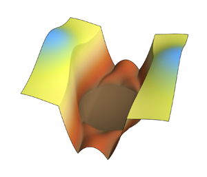
Figure 1. (a) Sketch of a porous medium saturated by two immiscible phases, highlighting the characteristic length and the corresponding interfaces. (b) Periodic representation of the microstructure and periodic unit cell.
Directing the attention to the fluid–solid interface, it is assumed that the no-slip boundary condition is applicable, i.e.
 \begin{equation} \boldsymbol{v}_\alpha =\boldsymbol{0},\quad \text{at }\mathscr{A}_{\alpha \sigma}, \quad \alpha=\beta,\gamma. \end{equation}
To simplify the problem, it is further assumed that there is no three-phase contact line; consequently the above equations are sufficient to describe the interfacial transport phenomena under consideration. Certainly, the pore-scale problem statement requires providing the boundary conditions for the pressure and velocity at the macroscopic boundaries. However, this information is not required for the derivation of the UM that follows and it is not presented here for the sake of brevity.
3. Essentials of the volume averaging
The derivation of the upscaled mass and momentum balance equations is performed using elements of the volume averaging method (Whitaker Reference Whitaker1999) and Green's formula from the adjoint homogenization technique (Bottaro Reference Bottaro2019). The purpose of this section is to provide the essential elements of this upscaling approach. To this end, consider an averaging domain  $\mathscr {V}$ (of constant measure $V$) containing portions of all the phases involved in the system. Assuming that there exists a disparity between the largest characteristic length scale associated with the pore scale ( $\ell _p= \max (\ell _\kappa$), $\ell _\kappa$ representing the characteristic length of the $\kappa$-phase, $\kappa =\beta,\gamma,\sigma$, see figure 1(a) and the smallest macroscopic length scale ( $L$), it follows that, in order for $\mathscr {V}$ to be representative, its characteristic length ( $r_0$) must be constrained according to (Bear Reference Bear2018)
 \begin{equation} \ell_p \ll r_0 \ll L. \end{equation}
On the basis of this constraint,  $\mathscr {V}$ can be denoted, in the rest of this work, as a REV. Moreover, in terms of this averaging domain, the superficial averaging operator can be introduced for a piecewise smooth (scalar or tensorial) function, $\psi$, defined everywhere
 \begin{equation} \langle \psi \rangle = \frac{1}{V}\int_{\mathscr{V}}\psi\,{{\rm d}}V. \end{equation}
For the case in which  $\psi$ is only defined in the $\alpha$-phase ( $\alpha =\beta,\gamma$), the above expression yields (Whitaker Reference Whitaker1999)
 \begin{equation} \langle \psi_\alpha \rangle_\alpha = \frac{1}{V}\int_{\mathscr{V}_\alpha} \psi_\alpha\,{{\rm d}}V. \end{equation}
Here  $\mathscr{V}_\alpha$ represents the space occupied by the $\alpha$-phase within $\mathscr{V}$. In addition, the intrinsic averaging operator is defined as
 \begin{equation} \langle \psi_\alpha \rangle^{\alpha} = \frac{1}{V_\alpha}\int_{\mathscr{V}_\alpha} \psi_\alpha\,{{\rm d}}V. \end{equation}
In the following, the volume fraction of the fluid phases in the REV is denoted as
 \begin{equation} \varepsilon_\alpha =\langle 1 \rangle_\alpha = \frac{V_\alpha}{V}, \end{equation}
and the two averages are related by  $\langle \psi _\alpha \rangle _\alpha =\varepsilon _\alpha \langle \psi _\alpha \rangle ^{\alpha }$.
Furthermore, the application of the spatial averaging operators to the pore-scale equations often requires interchanging temporal differentiation and spatial differentiation. This is achieved by means of the general transport theorem (Slattery Reference Slattery1999)
 \begin{equation} \frac{{{\rm d}} \langle \psi_\alpha \rangle_\alpha}{{{\rm d}}t} = \left\langle \frac{\partial \psi_\alpha}{\partial t} \right\rangle_\alpha + \frac{1}{V}\int_{\mathscr{A}_\alpha} \boldsymbol{n}_\alpha\boldsymbol{\cdot} \psi_\alpha\boldsymbol{w}\,{{\rm d}}A. \end{equation}
Here,  $\mathscr {A}_\alpha = \mathscr {A}_{\alpha \sigma }+\mathscr {A}_{\beta \gamma }$ denotes the bounding surfaces of $\mathscr {V}_\alpha$, and $\boldsymbol {n}_\alpha$ represents the unit normal vector at $\mathscr {A}_\alpha$ pointing out of $\mathscr {V}_\alpha$, whereas $\boldsymbol {w}$ is the speed of displacement of $\mathscr {A}_\alpha$. In addition, the interchange of spatial differentiation and integration is possible using the spatial averaging theorem, which, for the gradient operator, takes the form (see, for example, Howes & Whitaker (Reference Howes and Whitaker1985))
 \begin{equation} \left\langle \boldsymbol{\nabla} \psi_\alpha\right\rangle_\alpha = \boldsymbol{\nabla} \left\langle \psi_\alpha\right\rangle_\alpha +\frac{1}{V} \int_{\mathscr{A}_\alpha} \boldsymbol{n}_\alpha \psi_\alpha\,{{\rm d}}A, \end{equation}
whereas an equivalent expression is applicable for the divergence operator. All these elements are employed below for the derivation of the upscaled mass balance equations.
A key element in the volume averaging method is the spatial decomposition of pore-scale quantities into their corresponding intrinsic averages and deviations (Gray Reference Gray1975)
 \begin{equation} \psi_\alpha = \langle \psi_\alpha \rangle^{\alpha} + \tilde{\psi}_\alpha. \end{equation}
In the volume averaging context, average quantities are slow-varying fields, and pore-scale properties, such as the spatial deviations, are fast-varying fields. The determination of the deviation quantities is usually done in a periodic unit cell where they are assumed to be periodic at the inlet and outlet surfaces. In contrast, in the homogenization technique, the derivations commence by considering the pore-scale equations in a periodic unit cell and then performing the corresponding expansions and simplifications in terms of length scale constraints. Both upscaling methods share many elements in common as detailed by Davit et al. (Reference Davit2013) and it is thus pertinent to use elements from both approaches. In particular, the derivation of the upscaled equations for momentum transport can be advantageously carried out by following the adjoint homogenization technique outlined by Bottaro (Reference Bottaro2019). This consists of combining the pore-scale flow problem with the adjoint Green's functions velocity pairs by means of a Green's formula (Haberman Reference Haberman2012). For a scalar field  $a_\alpha$, two vector fields $\boldsymbol {a}_\alpha$ and $\boldsymbol {b}_\alpha$, and a second-order tensor field $\textsf{B}_\alpha$, arbitrarily defined in the $\alpha$-phase ( $\alpha =\beta,\gamma$), and having the appropriate required regularities, $\boldsymbol {a}_\alpha$ and $\textsf{B}_\alpha$ being solenoidal, this formula can be written as (see the proof in Appendix A)
 \begin{align} & \int_{\mathscr{V}_\alpha} \left[\boldsymbol{a}_\alpha \boldsymbol{\cdot} \left( -\boldsymbol{\nabla}\boldsymbol{b}_\alpha+ \nabla^{2} \textsf{B}_\alpha \right) - \left(-\boldsymbol{\nabla} a_\alpha+\nabla^{2} \boldsymbol{a}_\alpha\right)\boldsymbol{\cdot}\textsf{B}_\alpha\right]{{\rm d}}V \nonumber\\ &\quad =\int_{\mathscr{A}_\alpha} \left[\boldsymbol{a}_\alpha \boldsymbol{\cdot} \left(\boldsymbol{n}_\alpha \boldsymbol{\cdot} \left(-\textsf{I}\boldsymbol{b}_\alpha + \boldsymbol{\nabla} \textsf{B}_\alpha + \boldsymbol{\nabla} \textsf{B}_\alpha^{{\rm T}1}\right)\right) \right.\nonumber\\ &\left.\qquad - \,\boldsymbol{n}_\alpha \boldsymbol{\cdot}\left(-\textsf{I} a_\alpha+ \boldsymbol{\nabla}\boldsymbol{a}_\alpha+\boldsymbol{\nabla} \boldsymbol{a}_\alpha^{\rm T}\right)\boldsymbol{\cdot} \textsf{B}_\alpha\right]{{\rm d}}A. \end{align}
Here, the superscript T1 denotes the transpose of a third-order tensor that permutes the two first indices, i.e.  $(\boldsymbol {\nabla } \textsf{B}_\alpha ^{{\rm T}1})_{ijk}=(\boldsymbol {\nabla } \textsf{B}_\alpha )_{jik}$. This approach allows deriving a solution of the pore-scale problem. Application of the averaging operator to the formal solution of the pore-scale velocity yields the macroscopic momentum transport equations.
4. Upscaled mass balance equation
The derivation starts by directing the attention to the pore-scale mass balance equation for each phase given in (2.1a). Application of the superficial averaging operator (see (3.2b)) to this equation, and use of the spatial averaging theorem, yields ( $\alpha = \beta, \gamma$)
 \begin{equation} \boldsymbol{\nabla} \boldsymbol{\cdot} \left\langle \boldsymbol{v}_\alpha \right\rangle_\alpha +\frac{1}{V}\int_{\mathscr{A}_\alpha} \boldsymbol{n}_\alpha \boldsymbol{\cdot} \boldsymbol{v}_\alpha\,{{\rm d}}A=0. \end{equation}
Taking into account the no slip boundary condition at  $\mathscr {A}_{\alpha \sigma }$ as well as (2.1c), allows rewriting this last expression as
 \begin{equation} \boldsymbol{\nabla} \boldsymbol{\cdot} \left\langle \boldsymbol{v}_\alpha \right\rangle_\alpha +\frac{1}{V}\int_{\mathscr{A}_{\beta \gamma}} \boldsymbol{n}_\alpha \boldsymbol{\cdot} \boldsymbol{w}\,{{\rm d}}A=0. \end{equation}
The last term on the left-hand side of this equation can be further developed by making use of the general transport theorem (3.4) in which  $\psi _\alpha =1$, taking into account the fact that the solid phase is supposed to be immobile, that the averaging domain, $\mathscr {V}$, is fixed and the definition of the volume fraction of the $\alpha$-phase is as given in (3.3). This yields
 \begin{equation} \frac{\partial \varepsilon_\alpha}{\partial t} + \boldsymbol{\nabla} \boldsymbol{\cdot} \left\langle \boldsymbol{v}_\alpha \right\rangle_\alpha =0,\quad \alpha=\beta, \gamma. \end{equation}
These equations correspond to those originally derived by Whitaker (Reference Whitaker1986) and represent the final closed form of the upscaled mass balance equations.
5. Upscaled momentum balance equations
As mentioned in § 3, it is convenient to begin the derivation of the upscaled momentum balance equations by writing the pore-scale conservation equations in a periodic unit cell as the one sketched in figure 1(b) that is representative of the phases distribution in the real system. In this simplified domain, it is pertinent to spatially decompose the pressure into its intrinsic average and deviations, so that the governing equations for mass and momentum balance in a unit cell can be written as ( $\alpha =\beta, \gamma$)
 $$\begin{gather} \boldsymbol{\nabla} \boldsymbol{\cdot} \boldsymbol{v}_\alpha =0, \quad \text{in } \mathscr{V}_\alpha, \end{gather}$$
 $$\begin{gather}\boldsymbol{0}={-} \boldsymbol{\nabla} \tilde{p}_\alpha + \mu_\alpha \nabla^{2} \boldsymbol{v}_\alpha - (\boldsymbol{\nabla} \langle p_\alpha\rangle^{\alpha} - \rho_\alpha \boldsymbol{g}),\quad \text{in } \mathscr{V}_\alpha. \end{gather}$$
In addition, the interfacial boundary conditions are expressed as follows:
 \begin{gather} \boldsymbol{v}_\beta = \boldsymbol{v}_\gamma,\quad \text{at } \mathscr{A}_{\beta \gamma},\end{gather}
 \begin{gather} \boldsymbol{n}_{\beta
\gamma} \boldsymbol{\cdot}
[-\textsf{I} \tilde{p}_\beta
+\mu_\beta (\boldsymbol{\nabla} \boldsymbol{v}_\beta +
\boldsymbol{\nabla} \boldsymbol{v}_\beta^{\rm T})]
= \boldsymbol{n}_{\beta \gamma} \boldsymbol{\cdot}
[-\textsf{I} \tilde{p}_\gamma
+\mu_\gamma (\boldsymbol{\nabla} \boldsymbol{v}_\gamma +
\boldsymbol{\nabla} \boldsymbol{v}_\gamma^{\rm T})]
\nonumber\\ \hspace{9pc} +\,\boldsymbol{n}_{\beta \gamma} (
\langle p_\beta \rangle^{\beta} - \langle p_\gamma
\rangle^{\gamma}) \nonumber\\ \hspace{14pc}+\,2 \gamma H
\boldsymbol{n}_{\beta \gamma}+\boldsymbol{\nabla}_s \gamma,
\quad \text{at }\mathscr{A}_{\beta\gamma},
\end{gather}
\begin{gather} \boldsymbol{n}_{\beta
\gamma} \boldsymbol{\cdot}
[-\textsf{I} \tilde{p}_\beta
+\mu_\beta (\boldsymbol{\nabla} \boldsymbol{v}_\beta +
\boldsymbol{\nabla} \boldsymbol{v}_\beta^{\rm T})]
= \boldsymbol{n}_{\beta \gamma} \boldsymbol{\cdot}
[-\textsf{I} \tilde{p}_\gamma
+\mu_\gamma (\boldsymbol{\nabla} \boldsymbol{v}_\gamma +
\boldsymbol{\nabla} \boldsymbol{v}_\gamma^{\rm T})]
\nonumber\\ \hspace{9pc} +\,\boldsymbol{n}_{\beta \gamma} (
\langle p_\beta \rangle^{\beta} - \langle p_\gamma
\rangle^{\gamma}) \nonumber\\ \hspace{14pc}+\,2 \gamma H
\boldsymbol{n}_{\beta \gamma}+\boldsymbol{\nabla}_s \gamma,
\quad \text{at }\mathscr{A}_{\beta\gamma},
\end{gather}
 \begin{gather} \boldsymbol{v}_\alpha =\boldsymbol{0}, \quad \text{at }\mathscr{A}_{\alpha \sigma}, \quad \alpha=\beta,\gamma. \end{gather}
In the rest of the derivations, the two fluid phases are assumed to be connected. Note that, to be compliant with periodicity, both interfaces  $\mathscr {A}_{\beta \gamma }$ and $\mathscr {A}_{\alpha \sigma }$ ( $\alpha =\beta,\gamma$) must also be periodic. Furthermore, at the scale level of the unit cell, it is reasonable to assume that the velocity and pressure deviations are periodic at the inlet and outlet surfaces of the unit cell, which means ( $\alpha = \beta, \gamma$),
 \begin{equation} \psi_\alpha (\boldsymbol{r}_\alpha) =\psi_\alpha (\boldsymbol{r}_\alpha+ \boldsymbol{l}_i),\quad i = 1,2,3; \quad \psi = \boldsymbol{v}, \tilde{p}. \end{equation}
Here,  $\boldsymbol {r}_\alpha$ is a position vector relative to a fixed coordinate system and $\boldsymbol {l}_i$ are the unit cell lattice vectors. It is important to stress that the periodicity assumption is convenient to make the flow problem solution local. Nevertheless, it is natural to expect that the range of applicability of the developments that follow extends beyond this hypothesis, which is barely met in practice.
Finally, in order for this problem to be well posed, the following average constraint for the pressure deviations is imposed ( $\alpha = \beta, \gamma$):
 \begin{equation} \langle \tilde{p}_\alpha \rangle^{\alpha} =0. \end{equation}
This constraint is a direct consequence of the separation of length scales given in (3.1), so that average quantities can be treated as constants within the unit cell.
From a mathematical point of view, several source terms can be identified in the above flow problem. Nevertheless, not all of them are independent from each other. For example, in order to guarantee that the fluid–fluid interface shape is periodic, the macroscopic pressure gradients in both phases must be equal (see the proof in Appendix B). Also, in the absence of any macroscopic forcing (pressure gradients and gravity effects) and for a constant surface tension, it follows that  $H$ must be constant. This point is relevant to be kept in mind in the macroscopic model that is derived below.
In order to derive the formal solution of this problem, the following two adjoint fundamental problems for the velocity Green's function pairs  $(\textsf{G}_\alpha, \boldsymbol {g}_\alpha )$ ( $\alpha = \beta, \gamma$) are considered:
 $$\begin{gather} \boldsymbol{\nabla} \boldsymbol{\cdot} \textsf{G}_\alpha = \boldsymbol{0}, \quad \text{in } \mathscr{V}_\alpha, \end{gather}$$
 $$\begin{gather}\boldsymbol{0}={-}\boldsymbol{\nabla} \boldsymbol{g}_\alpha +\mu_\alpha \nabla^{2} \textsf{G}_\alpha+ \delta (\boldsymbol{r}_\alpha -\boldsymbol{r}_{0 \alpha})\textsf{I}, \quad \text{in } \mathscr{V}_\alpha, \end{gather}$$
 $$\begin{gather}\textsf{G}_\beta = \textsf{G}_\gamma, \quad \text{at } \mathscr{A}_{\beta \gamma}, \end{gather}$$
 $$\begin{gather}
\hspace{-10pc}\boldsymbol{n}_{\beta\gamma}\boldsymbol{\cdot}
\left[-\textsf{I} \boldsymbol{g}_\beta
+\mu_\beta \left(\boldsymbol{\nabla}
\textsf{G}_\beta +\boldsymbol{\nabla}
\textsf{G}_\beta^{{\rm T}1}
\right)\right] \nonumber\\ \hspace{2pc} =
\boldsymbol{n}_{\beta\gamma}\boldsymbol{\cdot}
\left[-\textsf{I} \boldsymbol{g}_\gamma
+\mu_\gamma \left(\boldsymbol{\nabla}
\textsf{G}_\gamma +\boldsymbol{\nabla}
\textsf{G}_\gamma^{{\rm T}1} \right)
\right], \quad \text{at }\mathscr{A}_{\beta \gamma},
\end{gather}$$
$$\begin{gather}
\hspace{-10pc}\boldsymbol{n}_{\beta\gamma}\boldsymbol{\cdot}
\left[-\textsf{I} \boldsymbol{g}_\beta
+\mu_\beta \left(\boldsymbol{\nabla}
\textsf{G}_\beta +\boldsymbol{\nabla}
\textsf{G}_\beta^{{\rm T}1}
\right)\right] \nonumber\\ \hspace{2pc} =
\boldsymbol{n}_{\beta\gamma}\boldsymbol{\cdot}
\left[-\textsf{I} \boldsymbol{g}_\gamma
+\mu_\gamma \left(\boldsymbol{\nabla}
\textsf{G}_\gamma +\boldsymbol{\nabla}
\textsf{G}_\gamma^{{\rm T}1} \right)
\right], \quad \text{at }\mathscr{A}_{\beta \gamma},
\end{gather}$$
 $$\begin{gather} \textsf{G}_\alpha =\boldsymbol{0}, \quad \text{at }\mathscr A_{\alpha \sigma}, \end{gather}$$
 $$\begin{gather}\psi_\alpha (\boldsymbol{r}_\alpha) = \psi_\alpha (\boldsymbol{r}_\alpha+\boldsymbol{l}_i), \quad i=1,2,3; \quad \psi = \textsf{G}, \boldsymbol{g}, \end{gather}$$
 $$\begin{gather}
\boldsymbol{g}_\alpha=\mathbf{0} \ \text{at}\ \boldsymbol{r}_{\alpha}^0.
\end{gather}$$
$$\begin{gather}
\boldsymbol{g}_\alpha=\mathbf{0} \ \text{at}\ \boldsymbol{r}_{\alpha}^0.
\end{gather}$$
In the above equations,  $\textsf{G}_\alpha$ and $\boldsymbol {g}_\alpha$ are the Green's functions that map the influence of sources located at a given position $\boldsymbol {r}_{0\alpha }$ onto the velocity and pressure deviations located at $\boldsymbol {r}_\alpha$. Moreover, $\delta (\boldsymbol {r}_\alpha -\boldsymbol {r}_{0\alpha })$ represents the Dirac delta function centred at $\boldsymbol {r}_{0\alpha }$. Although not explicitly written for the sake of simplicity in notation, the velocity Green's function pairs depend on $\boldsymbol {r}_\alpha$ and $\boldsymbol {r}_{0\alpha }$. Moreover, in (5.2) the derivation and integration operations are taken with respect to $\boldsymbol {r}_{\alpha }$. The last of equations (5.2) sets a point value (at $\boldsymbol{r}_\alpha^0$) to $\boldsymbol{g}_\alpha$ to have a well-posed problem, as should have been specified in equation (3.12d) in Lasseux, Valdés‐Parada & Bottaro (Reference Lasseux, Valdés-Parada and Bottaro2021), instead of a zero average. Note that the statement of this problem requires knowledge of $\mathscr {A}_{\beta \gamma }$. This information can be acquired from the flow problem solution at the pore scale or from experimental data.
At this point, the following decompositions shall be introduced ( $\alpha = \beta, \gamma$):
 $$\begin{gather} \textsf{G}_\alpha = \textsf{G}_{\alpha \beta}+ \textsf{G}_{\alpha \gamma }, \end{gather}$$
 $$\begin{gather}\boldsymbol{g}_\alpha = \boldsymbol{g}_{\alpha \beta }+ \boldsymbol{g}_{\alpha \gamma }. \end{gather}$$
Substituting these expressions into (5.2) and taking into account linearity, the following two subproblems can be written ( $\alpha=\beta, \gamma$).
Problem I:
 $$\begin{gather} \boldsymbol{\nabla} \boldsymbol{\cdot} \textsf{G}_{\alpha \beta} = \boldsymbol{0},\quad \text{in } \mathscr{V}_\alpha, \end{gather}$$
 $$\begin{gather}\boldsymbol{0}={-}\boldsymbol{\nabla} \boldsymbol{g}_{\alpha \beta }+\mu_\alpha \nabla^{2} \textsf{G}_{\alpha \beta }+ \delta^{K}_{\alpha \beta} \delta (\boldsymbol{r}_\alpha -\boldsymbol{r}_{0 \alpha})\textsf{I}, \quad \text{in } \mathscr{V}_\alpha, \end{gather}$$
 $$\begin{gather}\textsf{G}_{\beta \beta} = \textsf{G}_{\gamma \beta},\quad \text{at } \mathscr{A}_{\beta \gamma}, \end{gather}$$
 $$\begin{gather}
\hspace{-10pc}\boldsymbol{n}_{\beta\gamma}\boldsymbol{\cdot} [
-\textsf{I} \boldsymbol{g}_{\beta\beta} +
\mu_\beta( \boldsymbol{\nabla}
\textsf{G}_{\beta\beta}
+\boldsymbol{\nabla}
\textsf{G}_{\beta\beta }^{{\rm T}1} ) ]
\nonumber\\ \hspace{2pc}
=\boldsymbol{n}_{\beta\gamma}\boldsymbol{\cdot} [
-\textsf{I} \boldsymbol{g}_{ \gamma
\beta} +\mu_\gamma( \boldsymbol{\nabla}
\textsf{G}_{\gamma \beta}
+\boldsymbol{\nabla} \textsf{G}_{ \gamma
\beta}^{{\rm T}1})], \quad \text{at } \mathscr{A}_{\beta
\gamma}, \end{gather}$$
$$\begin{gather}
\hspace{-10pc}\boldsymbol{n}_{\beta\gamma}\boldsymbol{\cdot} [
-\textsf{I} \boldsymbol{g}_{\beta\beta} +
\mu_\beta( \boldsymbol{\nabla}
\textsf{G}_{\beta\beta}
+\boldsymbol{\nabla}
\textsf{G}_{\beta\beta }^{{\rm T}1} ) ]
\nonumber\\ \hspace{2pc}
=\boldsymbol{n}_{\beta\gamma}\boldsymbol{\cdot} [
-\textsf{I} \boldsymbol{g}_{ \gamma
\beta} +\mu_\gamma( \boldsymbol{\nabla}
\textsf{G}_{\gamma \beta}
+\boldsymbol{\nabla} \textsf{G}_{ \gamma
\beta}^{{\rm T}1})], \quad \text{at } \mathscr{A}_{\beta
\gamma}, \end{gather}$$
 $$\begin{gather} \textsf{G}_{\alpha \beta} =\boldsymbol{0}, \quad \text{at }\mathscr A_{\alpha \sigma}, \end{gather}$$
 $$\begin{gather}\psi_{\alpha \beta} (\boldsymbol{r}_\alpha) = \psi_{\alpha \beta} (\boldsymbol{r}_\alpha+\boldsymbol{l}_i), \quad i=1,2,3; \quad \psi = \textsf{G}, \boldsymbol{g}, \end{gather}$$
 $$\begin{gather}
\boldsymbol{g}_{\alpha \beta}= {0} \ \text{at}\ \boldsymbol{r}_{\alpha}^0.
\end{gather}$$
$$\begin{gather}
\boldsymbol{g}_{\alpha \beta}= {0} \ \text{at}\ \boldsymbol{r}_{\alpha}^0.
\end{gather}$$
Problem II:
 $$\begin{gather} \boldsymbol{\nabla} \boldsymbol{\cdot} \textsf{G}_{\alpha \gamma} = \boldsymbol{0}, \quad \text{in } \mathscr{V}_\alpha, \end{gather}$$
 $$\begin{gather}\boldsymbol{0}={-}\boldsymbol{\nabla} \boldsymbol{g}_{\alpha \gamma} +\mu_\alpha \nabla^{2} \textsf{G}_{\alpha \gamma}+ \delta^{K}_{\alpha \gamma} \delta (\boldsymbol{r}_\alpha -\boldsymbol{r}_{0 \alpha})\textsf{I}, \quad \text{in } \mathscr{V}_\alpha, \end{gather}$$
 $$\begin{gather}\textsf{G}_{\beta \gamma} = \textsf{G}_{\gamma \gamma}, \quad \text{at } \mathscr{A}_{\beta \gamma}, \end{gather}$$
 $$\begin{gather}
\hspace{-10pc}\boldsymbol{n}_{\beta\gamma}\boldsymbol{\cdot} [
-\textsf{I} \boldsymbol{g}_{\beta \gamma}
+\mu_\beta( \boldsymbol{\nabla}
\textsf{G}_{\beta \gamma}
+\boldsymbol{\nabla} \textsf{G}_{\beta
\gamma}^{{\rm T}1})] \nonumber\\ \hspace{2pc} =
\boldsymbol{n}_{\beta\gamma}\boldsymbol{\cdot} [
-\textsf{I} \boldsymbol{g}_{\gamma
\gamma} +\mu_\gamma( \boldsymbol{\nabla}
\textsf{G}_{\gamma\gamma}
+\boldsymbol{\nabla} \textsf{G}_{\gamma
\gamma}^{{\rm T}1})], \quad \text{at } \mathscr{A}_{\beta
\gamma}, \end{gather}$$
$$\begin{gather}
\hspace{-10pc}\boldsymbol{n}_{\beta\gamma}\boldsymbol{\cdot} [
-\textsf{I} \boldsymbol{g}_{\beta \gamma}
+\mu_\beta( \boldsymbol{\nabla}
\textsf{G}_{\beta \gamma}
+\boldsymbol{\nabla} \textsf{G}_{\beta
\gamma}^{{\rm T}1})] \nonumber\\ \hspace{2pc} =
\boldsymbol{n}_{\beta\gamma}\boldsymbol{\cdot} [
-\textsf{I} \boldsymbol{g}_{\gamma
\gamma} +\mu_\gamma( \boldsymbol{\nabla}
\textsf{G}_{\gamma\gamma}
+\boldsymbol{\nabla} \textsf{G}_{\gamma
\gamma}^{{\rm T}1})], \quad \text{at } \mathscr{A}_{\beta
\gamma}, \end{gather}$$
 $$\begin{gather} \textsf{G}_{\alpha \gamma} =\boldsymbol{0}, \quad \text{at }\mathscr A_{\alpha \sigma}, \end{gather}$$
 $$\begin{gather}\psi_{\alpha \gamma} (\boldsymbol{r}_\alpha) = \psi_{\alpha \gamma} (\boldsymbol{r}_\alpha+\boldsymbol{l}_i), \quad i=1,2,3; \quad \psi = \textsf{G}, \boldsymbol{g}, \end{gather}$$
 $$\begin{gather}
\boldsymbol{g}_{\alpha \gamma}= {0} \ \text{at}\ \boldsymbol{r}_{\alpha}^0
\end{gather}$$
$$\begin{gather}
\boldsymbol{g}_{\alpha \gamma}= {0} \ \text{at}\ \boldsymbol{r}_{\alpha}^0
\end{gather}$$
In (5.4b) and (5.5b),  $\delta ^{K}_{\alpha \kappa }$ denotes the Kronecker delta, so that, in problem I, the only source term is located in $\mathscr {V}_\beta$, whereas, in problem II, the source term is in $\mathscr {V}_\gamma$.
The two above Green's function problems may now be related to the flow problem given in (5.1) by means of Green's formula expressed in (3.7). Directing for the moment the attention to the  $\beta$-phase, this formula can be employed, in a first step, with $\boldsymbol {a}_\alpha =\boldsymbol {v}_\beta$, $a_\alpha =\tilde {p}_\beta /\mu _\beta$, $\boldsymbol {b}_\alpha =\boldsymbol {g}_{\beta \beta }$ and $\textsf{B}_\alpha =\mu _\beta \textsf{G}_{\beta \beta }$. Since all these fields are periodic, and taking into account the no slip conditions at $\mathscr {A}_{\beta \sigma }$, this leads to the following relationship:
 \begin{align} & \int_{\mathscr{V}_\beta} \left[\boldsymbol{v}_\beta \boldsymbol{\cdot} \left(-\boldsymbol{\nabla} \boldsymbol{g}_{\beta \beta} + \mu_\beta \nabla^{2} \textsf{G}_{\beta \beta} \right)-\left(-\boldsymbol{\nabla} \tilde{p}_\beta+ \mu_\beta \nabla^{2}\boldsymbol{v}_\beta\right) \boldsymbol{\cdot}\textsf{G}_{\beta \beta}\right]{{\rm d}}V \nonumber\\ &\quad =\int_{\mathscr{A}_{\beta\gamma}} \left\{\boldsymbol{v}_\beta \boldsymbol{\cdot}\left[\boldsymbol{n}_{\beta \gamma} \boldsymbol{\cdot} \left(-\textsf{I} \boldsymbol{g}_{\beta \beta} + \mu_\beta \left(\boldsymbol{\nabla} \textsf{G}_{\beta \beta} + \boldsymbol{\nabla} \textsf{G}_{\beta \beta}^{{\rm T}1} \right)\right)\right] \right.\nonumber\\ &\qquad \left.-\,\boldsymbol{n}_{\beta \gamma}\boldsymbol{\cdot}\left(-\tilde{p}_\beta\textsf{I}+ \mu_\beta \left(\boldsymbol{\nabla}\boldsymbol{v}_\beta+\boldsymbol{\nabla} \boldsymbol{v}_\beta^{\rm T}\right)\right)\boldsymbol{\cdot} \textsf{G}_{\beta \beta}\right\}{{\rm d}}A. \end{align}
In the above equation, the integration is performed with respect to  $\boldsymbol {r}_{0\beta }$. Substituting the corresponding differential equations in the left-hand side of the above equation yields
 \begin{align} \boldsymbol{v}_\beta &={-} \left( \boldsymbol{\nabla} \langle p_\beta\rangle^{\beta} - \rho_\beta \boldsymbol{g}\right)\boldsymbol{\cdot} \int_{\mathscr{V}_\beta} \textsf{G}_{\beta \beta}{{\rm d}}V \nonumber\\ &\quad -\int_{\mathscr{A}_{\beta\gamma}} \left\{\boldsymbol{v}_\beta \boldsymbol{\cdot} \left[\boldsymbol{n}_{\beta\gamma} \boldsymbol{\cdot} \left( -\textsf{I}\boldsymbol{g}_{\beta \beta} + \mu_\beta\left( \boldsymbol{\nabla} \textsf{G}_{\beta \beta} + \boldsymbol{\nabla} \textsf{G}_{\beta \beta}^{{\rm T}1} \right) \right)\right] \right. \nonumber\\ &\quad \left.-\,\boldsymbol{n}_{\beta\gamma} \boldsymbol{\cdot}\left(- \tilde{p}_\beta \textsf{I} + \mu_\beta \left( \boldsymbol{\nabla}\boldsymbol{v}_\beta+\boldsymbol{\nabla} \boldsymbol{v}_\beta^{\rm T}\right) \right)\boldsymbol{\cdot} \textsf{G}_{\beta \beta}\right\}{{\rm d}}A. \end{align}
 In this last expression, the filtration property of the Dirac delta function was used as well as the assumption of spatial invariance of volume-averaged quantities within the unit cell. The superficial average, as defined in (3.2a) (integration with respect to  $\boldsymbol{r}_\alpha$), can now be applied to this equation and the last term on the right-hand side of (5.7) can be further reformulated after substitution of the interfacial boundary conditions given in (5.1c), (5.1d) and (5.4c), (5.4d). This leads to the following expression of $\langle\boldsymbol{v}_\beta\rangle_\beta$:
 \begin{align}
&\langle \boldsymbol{v}_\beta\rangle_\beta
=- \left( \nabla \langle p_\beta\rangle^\beta - \rho_\beta \boldsymbol{g}\right)\boldsymbol{\cdot} \frac{1}{V}\int\limits_{\mathscr{V}_\beta}\int\limits_{\mathscr{V}_\beta} \boldsymbol{\mathsf{G}}_{\beta \beta} ~{\rm d}V {\rm d}V
\nonumber \\
& - \frac{1}{V} \int\limits_{\mathscr{A}_{\beta\gamma}}
\left\{
\boldsymbol{v}_\gamma \boldsymbol{\cdot} \left[ \boldsymbol{n}_{\beta\gamma} \boldsymbol{\cdot} \left( -\boldsymbol{\mathsf{I}}\int\limits_{\mathscr{V}_\gamma}\boldsymbol{g}_{\gamma \beta}~{\rm d}V + \mu_\gamma\left( \nabla \int\limits_{\mathscr{V}_\gamma}\boldsymbol{\mathsf{G}}_{\gamma \beta}~{\rm d}V + \left(\nabla \int\limits_{\mathscr{V}_\gamma}\boldsymbol{\mathsf{G}}_{\gamma \beta}~{\rm d}V \right)^{{\rm T}1} \right) \right)
\right]\right. \nonumber \\
& \left.\qquad \qquad
-\boldsymbol{n}_{\beta\gamma} \boldsymbol{\cdot} \left( -\tilde{p}_\gamma \boldsymbol{\mathsf{I}} + \mu_\gamma \left( \nabla\boldsymbol{v}_\gamma+\nabla \boldsymbol{v}_\gamma^{\rm T} \right) \right)\boldsymbol{\cdot} \int\limits_{\mathscr{V}_\gamma}\boldsymbol{\mathsf{G}}_{ \gamma\beta}~{\rm d}V
\right\}~{\rm d}A \nonumber \\ &
+\frac{1}{V} \int\limits_{\mathscr{A}_{\beta\gamma}}\left[ \left( 2 \gamma H \boldsymbol{n}_{\beta \gamma}+ \nabla_s \gamma \right)\boldsymbol{\cdot} \int\limits_{\mathscr{V}_\beta}\boldsymbol{\mathsf{G}}_{\beta \beta}~{\rm d}V\right]{\rm d}A.
\end{align}
\begin{align}
&\langle \boldsymbol{v}_\beta\rangle_\beta
=- \left( \nabla \langle p_\beta\rangle^\beta - \rho_\beta \boldsymbol{g}\right)\boldsymbol{\cdot} \frac{1}{V}\int\limits_{\mathscr{V}_\beta}\int\limits_{\mathscr{V}_\beta} \boldsymbol{\mathsf{G}}_{\beta \beta} ~{\rm d}V {\rm d}V
\nonumber \\
& - \frac{1}{V} \int\limits_{\mathscr{A}_{\beta\gamma}}
\left\{
\boldsymbol{v}_\gamma \boldsymbol{\cdot} \left[ \boldsymbol{n}_{\beta\gamma} \boldsymbol{\cdot} \left( -\boldsymbol{\mathsf{I}}\int\limits_{\mathscr{V}_\gamma}\boldsymbol{g}_{\gamma \beta}~{\rm d}V + \mu_\gamma\left( \nabla \int\limits_{\mathscr{V}_\gamma}\boldsymbol{\mathsf{G}}_{\gamma \beta}~{\rm d}V + \left(\nabla \int\limits_{\mathscr{V}_\gamma}\boldsymbol{\mathsf{G}}_{\gamma \beta}~{\rm d}V \right)^{{\rm T}1} \right) \right)
\right]\right. \nonumber \\
& \left.\qquad \qquad
-\boldsymbol{n}_{\beta\gamma} \boldsymbol{\cdot} \left( -\tilde{p}_\gamma \boldsymbol{\mathsf{I}} + \mu_\gamma \left( \nabla\boldsymbol{v}_\gamma+\nabla \boldsymbol{v}_\gamma^{\rm T} \right) \right)\boldsymbol{\cdot} \int\limits_{\mathscr{V}_\gamma}\boldsymbol{\mathsf{G}}_{ \gamma\beta}~{\rm d}V
\right\}~{\rm d}A \nonumber \\ &
+\frac{1}{V} \int\limits_{\mathscr{A}_{\beta\gamma}}\left[ \left( 2 \gamma H \boldsymbol{n}_{\beta \gamma}+ \nabla_s \gamma \right)\boldsymbol{\cdot} \int\limits_{\mathscr{V}_\beta}\boldsymbol{\mathsf{G}}_{\beta \beta}~{\rm d}V\right]{\rm d}A.
\end{align}
Note that in this relationship, the average pressures were treated as constants within the unit cell and the fact that
 \begin{equation} \int_{\mathscr{A}_{\beta\gamma}} \boldsymbol{n}_{\beta \gamma} \boldsymbol{\cdot} \textsf{G}_{\beta \beta}\,{{\rm d}}A=\boldsymbol{0}, \end{equation}
was taken into account. This results from integration of (5.4a) over  $\mathscr {V}_\beta$ and use of the divergence theorem, taking into account the corresponding boundary conditions.
In a second step, Green's formula is used with  $\boldsymbol {a}_\alpha =\boldsymbol {v}_\gamma$, $a_\alpha =\tilde {p}_\gamma /\mu _\gamma$, $\boldsymbol {b}_\alpha =\boldsymbol {g}_{\gamma \beta }$ and $\textsf{B}_\alpha =\mu _\gamma \textsf{G}_{\gamma \beta }$. Repeating the derivations reported above leads to
 \begin{align} & \int_{\mathscr{A}_{\beta\gamma}} \left\{\boldsymbol{v}_\gamma \boldsymbol{\cdot} \left[\boldsymbol{n}_{\beta\gamma} \boldsymbol{\cdot} \left(-\textsf{I} \boldsymbol{g}_{\gamma \beta} +\mu_\gamma \left(\boldsymbol{\nabla} \textsf{G}_{\gamma \beta} + \boldsymbol{\nabla} \textsf{G}_{\gamma \beta}^{{\rm T}1} \right)\right)\right] \right. \nonumber\\ &\quad \left.-\,\boldsymbol{n}_{\beta\gamma} \boldsymbol{\cdot} \left( -\tilde{p}_\gamma \textsf{I} + \mu_\gamma \left( \boldsymbol{\nabla}\boldsymbol{v}_\gamma+\boldsymbol{\nabla} \boldsymbol{v}_\gamma^{\rm T}\right) \right)\boldsymbol{\cdot} \textsf{G}_{\gamma \beta}\right\}{{\rm d}}A= \left( \boldsymbol{\nabla} \langle p_\gamma\rangle^{\gamma} - \rho_\gamma \boldsymbol{g}\right)\boldsymbol{\cdot}\int_{\mathscr{V}_\gamma} \textsf{G}_{\gamma \beta}\,{{\rm d}}V. \end{align}
When the superficial average is applied to this equation and the result is substituted back into (5.8), the following expression of  $\langle\boldsymbol{v}_\beta\rangle_\beta$ is obtained:
 \begin{align}
\langle \boldsymbol{v}_\beta\rangle_\beta
=&-\frac{1}{V} \left( \nabla \langle p_\beta\rangle^\beta - \rho_\beta \boldsymbol{g}\right) \boldsymbol{\cdot} \int\limits_{\mathscr{V}_\beta} \int\limits_{\mathscr{V}_\beta} \boldsymbol{\mathsf{G}}_{\beta \beta} ~{\rm d}V {\rm d}V
\nonumber
\\
&-\frac{1}{V} \left( \nabla \langle p_\gamma\rangle^\gamma - \rho_\gamma \boldsymbol{g}\right)\boldsymbol{\cdot} \int\limits_{\mathscr{V}_\gamma}\int\limits_{\mathscr{V}_\gamma} \boldsymbol{\mathsf{G}}_{\gamma \beta} ~{\rm d}V {\rm d}V
\nonumber \\
&
+ \frac{1}{V} \int\limits_{\mathscr{A}_{\beta\gamma}}\left[ \left( 2 \gamma H \boldsymbol{n}_{\beta \gamma}+ \nabla_s \gamma \right) \boldsymbol{\cdot} \int\limits_{\mathscr{V}_\beta}\boldsymbol{\mathsf{G}}_{\beta \beta}~{\rm d}V\right] {\rm d}A.
\end{align}
\begin{align}
\langle \boldsymbol{v}_\beta\rangle_\beta
=&-\frac{1}{V} \left( \nabla \langle p_\beta\rangle^\beta - \rho_\beta \boldsymbol{g}\right) \boldsymbol{\cdot} \int\limits_{\mathscr{V}_\beta} \int\limits_{\mathscr{V}_\beta} \boldsymbol{\mathsf{G}}_{\beta \beta} ~{\rm d}V {\rm d}V
\nonumber
\\
&-\frac{1}{V} \left( \nabla \langle p_\gamma\rangle^\gamma - \rho_\gamma \boldsymbol{g}\right)\boldsymbol{\cdot} \int\limits_{\mathscr{V}_\gamma}\int\limits_{\mathscr{V}_\gamma} \boldsymbol{\mathsf{G}}_{\gamma \beta} ~{\rm d}V {\rm d}V
\nonumber \\
&
+ \frac{1}{V} \int\limits_{\mathscr{A}_{\beta\gamma}}\left[ \left( 2 \gamma H \boldsymbol{n}_{\beta \gamma}+ \nabla_s \gamma \right) \boldsymbol{\cdot} \int\limits_{\mathscr{V}_\beta}\boldsymbol{\mathsf{G}}_{\beta \beta}~{\rm d}V\right] {\rm d}A.
\end{align}
This result is consistent with the fact that the closure variables, which map the influence of the source terms onto the deviation quantities, are the integrals of the associated Green's function pairs, as anticipated by Wood & Valdés-Parada (Reference Wood and Valdés-Parada2013).
The overall development carried out to obtain the average form of  $\boldsymbol {v}_\beta$ can be repeated to derive the expression of the $\gamma$-phase macroscopic velocity, yielding
 \begin{align}
\langle\boldsymbol{v}_\gamma\rangle_\gamma
=&-\frac{1}{V} \left( \nabla \langle p_\gamma\rangle^\gamma - \rho_\gamma \boldsymbol{g}\right) \boldsymbol{\cdot} \int\limits_{\mathscr{V}_\gamma}\int\limits_{\mathscr{V}_\gamma} \boldsymbol{\mathsf{G}}_{\gamma \gamma} ~{\rm d}V {\rm d}V
\nonumber
\\
& -\frac{1}{V} \left( \nabla \langle p_\beta\rangle^\beta - \rho_\beta \boldsymbol{g}\right)\boldsymbol{\cdot} \int\limits_{\mathscr{V}_\beta}\int\limits_{\mathscr{V}_\beta} \boldsymbol{\mathsf{G}}_{\beta \gamma } ~{\rm d}V {\rm d}V
\nonumber \\
&
+ \frac{1}{V} \int\limits_{\mathscr{A}_{\beta\gamma}} \left[\left( 2 \gamma H \boldsymbol{n}_{\beta \gamma}+ \nabla_s \gamma \right) \boldsymbol{\cdot} \int\limits_{\mathscr{V}_\gamma}\boldsymbol{\mathsf{G}}_{\gamma \gamma}~{\rm d}V\right] {\rm d}A. \end{align}
\begin{align}
\langle\boldsymbol{v}_\gamma\rangle_\gamma
=&-\frac{1}{V} \left( \nabla \langle p_\gamma\rangle^\gamma - \rho_\gamma \boldsymbol{g}\right) \boldsymbol{\cdot} \int\limits_{\mathscr{V}_\gamma}\int\limits_{\mathscr{V}_\gamma} \boldsymbol{\mathsf{G}}_{\gamma \gamma} ~{\rm d}V {\rm d}V
\nonumber
\\
& -\frac{1}{V} \left( \nabla \langle p_\beta\rangle^\beta - \rho_\beta \boldsymbol{g}\right)\boldsymbol{\cdot} \int\limits_{\mathscr{V}_\beta}\int\limits_{\mathscr{V}_\beta} \boldsymbol{\mathsf{G}}_{\beta \gamma } ~{\rm d}V {\rm d}V
\nonumber \\
&
+ \frac{1}{V} \int\limits_{\mathscr{A}_{\beta\gamma}} \left[\left( 2 \gamma H \boldsymbol{n}_{\beta \gamma}+ \nabla_s \gamma \right) \boldsymbol{\cdot} \int\limits_{\mathscr{V}_\gamma}\boldsymbol{\mathsf{G}}_{\gamma \gamma}~{\rm d}V\right] {\rm d}A. \end{align}
These expressions are obtained on the basis of the initial hypotheses (creeping, steady, isothermal, immiscible and incompressible flow in the absence of interfacial mass transport and phase change) together with the existence of a periodic REV and under the length scales constraint expressed in (3.1). They do not require any other assumption and they can be rewritten as
 \begin{align} \langle \boldsymbol{v}_\beta \rangle_\beta &={-}\frac{\textsf{K}^{*{\rm T}}_{\beta \beta}}{\mu_\beta }\boldsymbol{\cdot} \left(\boldsymbol{\nabla} \langle p_\beta\rangle^{\beta} - \rho_\beta \boldsymbol{g}\right) -\frac{\textsf{K}^{*{\rm T}}_{\gamma \beta} }{\mu_\beta }\boldsymbol{\cdot} \left(\boldsymbol{\nabla} \langle p_\gamma\rangle^{\gamma} - \rho_\gamma \boldsymbol{g}\right) \nonumber\\ &\quad +\,\frac{1}{\mu_\beta V} \int_{\mathscr{A}_{\beta\gamma}} \left(2 \gamma H\boldsymbol{n}_{\beta \gamma}+ \boldsymbol{\nabla}_s \gamma \right) \boldsymbol{\cdot} \textsf{D}_{\beta \beta}\,{{\rm d}}A, \end{align}
 \begin{align} \langle \boldsymbol{v}_\gamma \rangle_\gamma &={-}\frac{\textsf{K}^{*{\rm T}}_{\gamma \gamma}}{\mu_\gamma }\boldsymbol{\cdot} \left( \boldsymbol{\nabla} \langle p_\gamma\rangle^{\gamma} - \rho_\gamma \boldsymbol{g}\right) -\frac{\textsf{K}^{*{\rm T}}_{\beta\gamma} }{\mu_\gamma }\boldsymbol{\cdot} \left( \boldsymbol{\nabla} \langle p_\beta\rangle^{\beta} - \rho_\beta\boldsymbol{g}\right) \nonumber\\ &\quad +\,\frac{1}{\mu_\gamma V} \int_{\mathscr{A}_{\beta\gamma}}\left( 2 \gamma H\boldsymbol{n}_{\beta \gamma}+ \boldsymbol{\nabla}_s \gamma \right) \boldsymbol{\cdot} \textsf{D}_{\gamma \gamma}\,{{\rm d}}A. \end{align}
Here, the following definitions were employed ( $\alpha, \kappa = \beta, \gamma$):
 $$\begin{gather} \textsf{D}_{\alpha \kappa} = \mu_\kappa \int_{\mathscr{V}_\alpha} \textsf{G}_{\alpha \kappa}\,{{\rm d}}V, \end{gather}$$
 $$\begin{gather}\textsf{K}^{*}_{\alpha \kappa}=\langle\textsf{D}_{\alpha \kappa}\rangle_\alpha. \end{gather}$$
Note that in (5.13a) the integration step is performed over  $\boldsymbol {r}_{0\alpha}$, whereas in (5.13b), the integration variable is $\boldsymbol {r}_\alpha$. In the above expressions, $\textsf{K}^{*}_{\alpha \alpha }$ ( $\alpha =\beta,\gamma$) represents the dominant permeability tensor in the $\alpha$-phase, whereas $\textsf{K}^{*}_{\alpha \kappa }$ ( $\alpha, \kappa =\beta, \gamma,\ \alpha \ne \kappa$) are the coupling permeability tensors as defined by Lasseux et al. (Reference Lasseux, Quintard and Whitaker1996). Moreover, $\textsf{D}_{\alpha \kappa }$ are the closure variables associated with the velocities. These variables solve the following boundary-value problems that result from volume integrating (5.4) and (5.5) ( $\alpha =\beta, \gamma$) with respect to $\boldsymbol {r}_{0\alpha }$, recalling that the derivation steps are performed over $\boldsymbol {r}_\alpha$.
Problem I:
 $$\begin{gather} \boldsymbol{\nabla} \boldsymbol{\cdot} \textsf{D}_{\alpha \beta} = \boldsymbol{0}, \quad \text{in } \mathscr{V}_\alpha, \end{gather}$$
 $$\begin{gather}\boldsymbol{0}={-}\boldsymbol{\nabla} \boldsymbol{d}_{\alpha \beta }+\nabla^{2} \textsf{D}_{\alpha \beta }+ \delta^{K}_{\alpha \beta} \textsf{I}, \quad \text{in } \mathscr{V}_\alpha, \end{gather}$$
 $$\begin{gather}\textsf{D}_{\beta \beta} = \textsf{D}_{\gamma \beta },\quad \text{at } \mathscr{A}_{\beta \gamma}, \end{gather}$$
 $$\begin{gather}
\hspace{-10pc}\boldsymbol{n}_{\beta\gamma}\boldsymbol{\cdot} \mu_\beta
[-\textsf{I} \boldsymbol{d}_{\beta\beta}
+( \boldsymbol{\nabla}
\textsf{D}_{\beta\beta}
+\boldsymbol{\nabla}
\textsf{D}_{\beta\beta }^{{\rm T}1} ) ]
\nonumber\\ \hspace{2pc}
=\boldsymbol{n}_{\beta\gamma}\boldsymbol{\cdot} \mu_\gamma
[-\textsf{I} \boldsymbol{d}_{\gamma \beta
} +(\boldsymbol{\nabla}
\textsf{D}_{\gamma \beta }
+\boldsymbol{\nabla} \textsf{D}_{\gamma
\beta }^{{\rm T}1} )],\quad \text{at } \mathscr{A}_{\beta
\gamma}, \end{gather}$$
$$\begin{gather}
\hspace{-10pc}\boldsymbol{n}_{\beta\gamma}\boldsymbol{\cdot} \mu_\beta
[-\textsf{I} \boldsymbol{d}_{\beta\beta}
+( \boldsymbol{\nabla}
\textsf{D}_{\beta\beta}
+\boldsymbol{\nabla}
\textsf{D}_{\beta\beta }^{{\rm T}1} ) ]
\nonumber\\ \hspace{2pc}
=\boldsymbol{n}_{\beta\gamma}\boldsymbol{\cdot} \mu_\gamma
[-\textsf{I} \boldsymbol{d}_{\gamma \beta
} +(\boldsymbol{\nabla}
\textsf{D}_{\gamma \beta }
+\boldsymbol{\nabla} \textsf{D}_{\gamma
\beta }^{{\rm T}1} )],\quad \text{at } \mathscr{A}_{\beta
\gamma}, \end{gather}$$
 $$\begin{gather} \textsf{D}_{\alpha \beta} =\boldsymbol{0}, \quad \text{at }\mathscr A_{\alpha \sigma}, \end{gather}$$
 $$\begin{gather}\psi_{\alpha \beta } (\boldsymbol{r}_\alpha) = \psi_{\alpha \beta } (\boldsymbol{r}_\alpha+\boldsymbol{l}_i), \quad i=1,2,3; \quad \psi = \textsf{D}, \boldsymbol{d}, \end{gather}$$
 $$\begin{gather}\boldsymbol{d}_{\alpha \beta}= {0} \ \text{at}\ \boldsymbol{r}_{\alpha}^0. \end{gather}$$
Problem II:
 $$\begin{gather} \boldsymbol{\nabla} \boldsymbol{\cdot} \textsf{D}_{\alpha \gamma} = \boldsymbol{0}, \quad \text{in } \mathscr{V}_\alpha, \end{gather}$$
 $$\begin{gather}\boldsymbol{0}={-}\boldsymbol{\nabla} \boldsymbol{d}_{\alpha \gamma}+\nabla^{2} \textsf{D}_{\alpha \gamma}+ \delta^{K}_{\alpha \gamma} \textsf{I}, \quad \text{in } \mathscr{V}_\alpha, \end{gather}$$
 $$\begin{gather}\textsf{D}_{\beta \gamma} = \textsf{D}_{\gamma \gamma}, \quad \text{at } \mathscr{A}_{\beta \gamma}, \end{gather}$$
 $$\begin{gather}
\hspace{-10pc}\boldsymbol{n}_{\beta\gamma}\boldsymbol{\cdot} \mu_\beta [
-\textsf{I} \boldsymbol{d}_{\beta \gamma}
+( \boldsymbol{\nabla} \textsf{D}_{\beta
\gamma} + \boldsymbol{\nabla}
\textsf{D}_{\beta \gamma}^{{\rm T}1})]
\nonumber\\ \hspace{2pc} =
\boldsymbol{n}_{\beta\gamma}\boldsymbol{\cdot} \mu_\gamma [
-\textsf{I} \boldsymbol{d}_{\gamma
\gamma} +( \boldsymbol{\nabla}
\textsf{D}_{\gamma\gamma} +
\boldsymbol{\nabla} \textsf{D}_{\gamma
\gamma}^{{\rm T}1} )],\quad \text{at } \mathscr{A}_{\beta
\gamma}, \end{gather}$$
$$\begin{gather}
\hspace{-10pc}\boldsymbol{n}_{\beta\gamma}\boldsymbol{\cdot} \mu_\beta [
-\textsf{I} \boldsymbol{d}_{\beta \gamma}
+( \boldsymbol{\nabla} \textsf{D}_{\beta
\gamma} + \boldsymbol{\nabla}
\textsf{D}_{\beta \gamma}^{{\rm T}1})]
\nonumber\\ \hspace{2pc} =
\boldsymbol{n}_{\beta\gamma}\boldsymbol{\cdot} \mu_\gamma [
-\textsf{I} \boldsymbol{d}_{\gamma
\gamma} +( \boldsymbol{\nabla}
\textsf{D}_{\gamma\gamma} +
\boldsymbol{\nabla} \textsf{D}_{\gamma
\gamma}^{{\rm T}1} )],\quad \text{at } \mathscr{A}_{\beta
\gamma}, \end{gather}$$
 $$\begin{gather} \textsf{D}_{\alpha \gamma} =\boldsymbol{0}, \quad \text{at }\mathscr A_{\alpha \sigma}, \end{gather}$$
 $$\begin{gather}\psi_{\alpha \gamma} (\boldsymbol{r}_\alpha) = \psi_{\alpha \gamma} (\boldsymbol{r}_\alpha+\boldsymbol{l}_i), \quad i=1,2,3; \quad \psi = \textsf{D}, \boldsymbol{d}, \end{gather}$$
 $$\begin{gather}\boldsymbol{d}_{\alpha \gamma}= {0} \ \text{at}\ \boldsymbol{r}_{\alpha}^0. \end{gather}$$
While writing these problems, the following additional definition was used: ( $\alpha, \kappa =\beta,\gamma$)
 \begin{equation} \boldsymbol{d}_{\alpha \kappa} = \frac{\mu_\kappa}{\mu_\alpha} \int_{\mathscr{V}_\alpha}\boldsymbol{g}_{\alpha \kappa}\,{{\rm d}}V. \end{equation}
Note that an alternative way of obtaining the expressions of the macroscopic velocities given in (5.12) is to combine closure problems I and II with the flow equations (5.1) using Green's formula (3.7).
Closure problems I and II are fully consistent with those obtained using the double-scale homogenization approach and reported by Auriault & Sanchez-Palencia (Reference Auriault and Sanchez-Palencia1986) (see also Auriault (Reference Auriault1987)), Bourgeat (Reference Bourgeat1997) (chapter 5) and recalled by Picchi & Battiato (Reference Picchi and Battiato2018). They also coincide with the closure problems provided by Lasseux et al. (Reference Lasseux, Quintard and Whitaker1996) using the volume averaging method. These authors demonstrated that, for the flow process under consideration, the dominant permeability tensors are symmetric (see also Lasseux & Valdés-Parada (Reference Lasseux and Valdés-Parada2017)). In addition, the following reciprocity condition was proved (Auriault Reference Auriault1987; Lasseux et al. Reference Lasseux, Quintard and Whitaker1996; Lasseux & Valdés-Parada Reference Lasseux and Valdés-Parada2017):
 \begin{equation} \mu_\beta \textsf{K}^{*}_{\beta \gamma} =\mu_\gamma \textsf{K}^{*{\rm T}}_{\gamma \beta}. \end{equation}
When these properties are introduced back into (5.12), the macroscopic momentum equations take the following final form:
 \begin{align} \langle \boldsymbol{v}_\beta \rangle_\beta &={-}\frac{\textsf{K}^{*}_{\beta \beta}}{\mu_\beta }\boldsymbol{\cdot} \left(\boldsymbol{\nabla} \langle p_\beta\rangle^{\beta} - \rho_\beta \boldsymbol{g}\right) -\frac{\textsf{K}^{*}_{ \beta \gamma} }{\mu_\gamma }\boldsymbol{\cdot} \left(\boldsymbol{\nabla} \langle p_\gamma\rangle^{\gamma} - \rho_\gamma \boldsymbol{g}\right) \nonumber\\ &\quad +\,\frac{1}{\mu_\beta V} \int_{\mathscr{A}_{\beta\gamma}}\left( 2 \gamma H\boldsymbol{n}_{\beta \gamma}+ \boldsymbol{\nabla}_s \gamma \right) \boldsymbol{\cdot} \textsf{D}_{\beta \beta}\,{{\rm d}}A, \end{align}
 \begin{align} \langle \boldsymbol{v}_\gamma \rangle_\gamma &={-}\frac{\textsf{K}^{*}_{\gamma \gamma}}{\mu_\gamma }\boldsymbol{\cdot} \left( \boldsymbol{\nabla} \langle p_\gamma\rangle^{\gamma} - \rho_\gamma \boldsymbol{g}\right) -\frac{\textsf{K}^{*}_{\gamma\beta} }{\mu_\beta }\boldsymbol{\cdot} \left(\boldsymbol{\nabla} \langle p_\beta\rangle^{\beta} - \rho_\beta \boldsymbol{g}\right) \nonumber\\ &\quad +\,\frac{1}{\mu_\gamma V} \int_{\mathscr{A}_{\beta\gamma}} \left( 2 \gamma H\boldsymbol{n}_{\beta \gamma}+ \boldsymbol{\nabla}_s \gamma \right) \boldsymbol{\cdot} \textsf{D}_{\gamma \gamma}\,{{\rm d}}A, \end{align}
and this is the salient result of the development. It must be emphasized that these macroscopic equations are applicable under the assumption of the existence of a periodic REV and the length scale constraint (3.1), in particular for an infinite periodic system. Moreover, this model is fully closed as all the coefficients in the above expressions can be evaluated from the solution of the two closure problems I and II, which requires the location of  $\mathscr {A}_{\beta \gamma }$ that satisfies the pore-scale flow problem.
In the absence of any macroscopic forcing and without interfacial tension gradient, the two first terms and the last integral interfacial term on the right-hand side of (5.18) are zero. Nevertheless, the interfacial integral term remains, suggesting that there is still a macroscopic velocity induced by this term, which would be unphysical under steady conditions. However, in the absence of any macroscopic force field, and with no surface tension gradient,  $H$ must be constant. Consequently, this remaining integral term is also zero because $\textsf{D}_{\alpha \alpha }$ ( $\alpha =\beta,\gamma$) is divergence-free, periodic and zero at $\mathscr {A}_{\beta \sigma }$. Moreover, despite the fact that periodicity implies equal macroscopic pressure gradients in both fluid phases (see Appendix B), the applicability of (5.18) is thought to extend beyond this hypothesis and, for this reason, the two macroscopic pressure gradients shall be kept distinct in these equations.
In addition to the viscous effects that are accounted for by the (dominant and coupling) Darcy terms represented by the first two terms on the right-hand side of (5.18), the last area integral term at  $\mathscr {A}_{\beta \gamma }$ expresses a compensation of surface tension to momentum transfer, that is only partly contained in the permeability tensors through their dependence upon the shape of this interface. This interfacial term is novel as, to the best of our knowledge, it has not been included in two-phase flow macroscopic models in porous media derived by upscaling and reported so far in the literature (Auriault & Sanchez-Palencia Reference Auriault and Sanchez-Palencia1986; Whitaker Reference Whitaker1986; Auriault Reference Auriault1987; Whitaker Reference Whitaker1994; Lasseux et al. Reference Lasseux, Quintard and Whitaker1996; Bourgeat Reference Bourgeat1997; Picchi & Battiato Reference Picchi and Battiato2018), despite the fact that, as mentioned above, the closure problems proposed in these references coincide with problems I and II. The new terms provide an explicit dependence of the momentum transport equations upon the interfacial area in a closed manner and are in agreement with previous expectations (Hassanizadeh & Gray Reference Hassanizadeh and Gray1993; Hilfer Reference Hilfer1998; Hilfer & Besserer Reference Hilfer and Besserer2000; Li et al. Reference Li, Pan and Miller2005; Niessner & Hassanizadeh Reference Niessner and Hassanizadeh2008; Niessner et al. Reference Niessner, Berg and Hassanizadeh2011).
More precisely, the difference in the macroscale momentum equations with respect to previous models can be explained as follows. In the model developed with the homogenization approach, a double-scale expansion in terms of  $\epsilon =\ell _p/L$ is performed. It leads to a boundary-value problem at the order $\epsilon ^{0}$ that involves non-local terms (i.e. with a characteristic length of variation $\ell _p$), in particular, a capillary source term in the boundary condition at $\mathscr {A}_{\beta \gamma }$ (see (4.14)–(4.18) in Auriault & Sanchez-Palencia (Reference Auriault and Sanchez-Palencia1986), (13)–(14) and associated boundary conditions in Auriault (Reference Auriault1987), (1.26) in Bourgeat (Reference Bourgeat1997) and appendix B in Picchi & Battiato (Reference Picchi and Battiato2018)). To obtain the closed macroscopic model, the solution (the closure) that is proposed is made local by not considering this capillary term as a source term for the solution on the velocity. However, it is included in the solution for the pressure (see (B.6) and (B.7) in Picchi & Battiato (Reference Picchi and Battiato2018)). In Auriault & Sanchez-Palencia (Reference Auriault and Sanchez-Palencia1986) (see (5.6) therein), the capillary source term was filtered out by considering the tangential projection of the boundary condition at the closure level. The normal component of this condition is said to be a ‘relationship between perturbations at a higher order that are not determined in the framework of homogenization’ (see remark 5.2, end of p. 150 in Auriault & Sanchez-Palencia (Reference Auriault and Sanchez-Palencia1986)). In the context of volume averaging, the capillary term in the boundary conditions of the closure problems is also finally dropped (see (2.10) and (2.11) in Lasseux et al. (Reference Lasseux, Quintard and Whitaker1996) that exactly coincide with the above problems I and II). The constraint put forth for such a simplification is
 \begin{equation} Ca_\alpha=\frac{\mu_\alpha v_\alpha}{\gamma}\ll 1,\quad \alpha=\beta,\gamma, \end{equation}
where  $Ca_\alpha$ is the capillary number associated with the $\alpha$-phase and $v_\alpha$ the order of magnitude estimate of $\boldsymbol {v}_\alpha$. In fact, on the basis of this argument, it was shown that the two boundary terms $\boldsymbol {n}_{\beta \gamma } (\langle p_\beta \rangle ^{\beta } - \langle p_\gamma \rangle ^{\gamma })+2 \gamma H \boldsymbol {n}_{\beta \gamma }$ can be simplified as follows (see details in Torres (Reference Torres1987) and Whitaker (Reference Whitaker1994)):
 \begin{equation} \boldsymbol{n}_{\beta \gamma} \left(\langle p_\beta \rangle^{\beta} - \langle p_\gamma \rangle^{\gamma} \right)+2 \gamma H \boldsymbol{n}_{\beta \gamma} \simeq 2\gamma\tilde{H} \boldsymbol{n}_{\beta \gamma},\end{equation}
where  $\tilde {H}=H-\langle H\rangle _{\beta \gamma }$, $\langle H\rangle _{\beta \gamma }=({1}/{A_{\beta \gamma }})\int _{\mathscr {A}_{\beta \gamma }}H\,{{\rm d}}A$ and where $A_{\beta \gamma }$ is the measure of $\mathscr {A}_{\beta \gamma }$. However, as cautiously pointed out by Whitaker (Reference Whitaker1994) (see (4.25) therein and the associated remark), neglecting this remaining capillary term in the boundary condition at $\mathscr {A}_{\beta \gamma }$ on the basis of the constraint (5.19) is ‘in the nature of a hypothesis’. At this point, it is worth noticing that $H$ can be replaced by $\tilde {H}$ in the macroscopic momentum equations (5.18) because $\langle H\rangle _{\beta \gamma }$ can be treated as a constant in the area integral over $\mathscr {A}_{\beta \gamma }$, $\textsf{D}_{\beta \gamma }$ is solenoidal, periodic and zero at $\mathscr {A}_{\beta \sigma }$. Taking into account the remark made above just after (5.8), it follows that the approximation (5.20) with its associated constraint (5.19) is unnecessary in the present development.
It is now of interest to explore whether the constraint expressed in (5.19) is consistent with a negligible contribution of the interfacial term resulting from surface tension effects to the average velocity in the  $\alpha$-phase in (5.18). To this end, an order of magnitude estimate of this term may be performed, and this leads to ( $\alpha=\beta,\gamma$)
 \begin{equation} \frac{1}{\mu_\alpha V} \int_{\mathscr{A}_{\beta\gamma}} \left(2 \gamma H \boldsymbol{n}_{\beta \gamma} + \boldsymbol{\nabla}_s \gamma \right) \boldsymbol{\cdot} \textsf{D}_{\alpha \alpha}\,{{\rm d}}A=\boldsymbol{O} \left(\frac{\gamma K_{\alpha\alpha}}{\mu_\alpha \varepsilon_\alpha\ell_p} a_{\beta \gamma} \right). \end{equation}
Here,  $a_{\beta \gamma }$ denotes the order of magnitude estimate of the fluid–fluid interfacial area per unit volume of the porous medium, $a_{\beta \gamma }=\boldsymbol {O}(A_{\beta \gamma }/V )$, whereas $H$ and $\boldsymbol {\nabla }_s$ are assumed to scale as the inverse of the pore-scale characteristic length, $1/\ell _p$. In addition, the order of magnitude estimate for $\textsf{D}_{\alpha \alpha }$, which is the same as $\langle \textsf{D}_{\alpha \alpha }\rangle ^{\alpha }=\langle \textsf{D}_{\alpha \alpha }\rangle _\alpha /\varepsilon _\alpha$, was extracted from the definition of $\textsf{K}_{\alpha \alpha }$ given in (5.13b), yielding $\textsf{D}_{\alpha \alpha }=\boldsymbol {O}(K_{\alpha \alpha }/\varepsilon _\alpha )$, $K_{\alpha \alpha }$ denoting the order of magnitude estimate of $\textsf{K}_{\alpha \alpha }$. Noticing that $\langle \boldsymbol {v}_\alpha \rangle _\alpha =\varepsilon _\alpha \langle \boldsymbol {v}_\alpha \rangle ^{\alpha }=\varepsilon _\alpha \boldsymbol {O}(v_\alpha )$, where again $v_\alpha =\boldsymbol {O}(\boldsymbol {v}_\alpha )$, it follows that the contribution of the interfacial term to the $\alpha$-phase macroscopic momentum transfer can be reasonably neglected when the following constraint is satisfied:
 \begin{equation} \frac{\varepsilon_\alpha^{2}\ell_p}{a_{\beta \gamma} K_{\alpha\alpha}}{Ca}_\alpha\gg 1. \end{equation}
Since the prefactor of  $Ca_\alpha$ on the left-hand side of the last expression is not expected to be systematically much larger than unity, this constraint is obviously quite different from (5.19) that was assumed by Whitaker (Reference Whitaker1994) and Lasseux et al. (Reference Lasseux, Quintard and Whitaker1996) to reach a macroscopic model for momentum that coincides with (5.18) in which the area integral terms due to capillary effects are negligible.
In § 6, two-phase flow numerical results are reported with the aim of validating the macroscopic model derived in this work and illustrating, in a particular example, the importance of the interfacial term in the upscaled momentum equations with respect to the above constraint.
6. Numerical simulations
This section is dedicated to a validation of the macroscopic model that is performed by first carrying out DNS of the pore-scale flow problem (5.1) using a boundary integral element method (BIEM). The solution provides the location and shape of  $\mathscr {A}_{\beta \gamma }$ that satisfies the pore-scale equilibrium, as well as the velocity (and pressure deviation) fields in each phase from which the average velocities can be computed. Second, the two closure problems I and II are solved with the same BIEM procedure, allowing the computation of the required permeability coefficients and the interfacial integral terms representing the contribution of capillary effects to momentum transfer. The average velocities predicted from the upscaled model (UM) are then computed from (5.18) and further compared with the numerical averaged fields obtained from DNS. This is carried out in a two-dimensional model configuration in the absence of surface tension gradient and ignoring gravity, i.e. $\boldsymbol {\nabla }_s\gamma =\boldsymbol {0}$ and $\boldsymbol {g}=\boldsymbol {0}$.
6.1. Configuration and dimensionless forms
The two-dimensional configuration under consideration is made of a periodic square pattern of parallel solid cylinders of circular cross-section, a unit cell of which is depicted in figure 2. The  $\beta$-phase is supposed to be the wetting phase, flowing under the form of a connected periodic layer attached to the cylinders at the core of the unit cell, whereas the non-wetting $\gamma$-phase flows in shell periodic layers (see figure 2). A macroscopic pressure gradient is only applied in the $x$-direction in each phase ( ${\partial \langle p_\alpha \rangle ^{\alpha }}/{\partial y}=0$, $\alpha =\beta, \gamma$). As shown in Appendix B, periodicity requires adopting a common value for the macroscopic pressure gradients in both phases, namely
 \begin{equation} \frac{\partial\langle p_\alpha\rangle^{\alpha}}{\partial x}={-}h,\quad \alpha=\beta, \gamma. \end{equation}
Figure 2. Configuration of the two-dimensional structure considered for the numerical simulations. It consists of a square pattern of parallel cylinders of circular cross-section (on the left) whose corresponding periodic unit cell is represented on the right. The wetting  $\beta$-phase is flowing as a core layer attached to the cylinders and the non-wetting $\gamma$-phase is flowing as a shell layer.
For convenience, the pore-scale problem, the two closure problems and the macroscopic momentum equations are made dimensionless employing the following scalings (dimensionless quantities are denoted with the superscript  $^{*}$; $\alpha, \kappa =\beta, \gamma$):
 \begin{equation} \left.\begin{gathered} \boldsymbol{r}^{*}=\frac{\boldsymbol{r}}{\ell},\quad \boldsymbol{v}_\alpha^{*}=\frac{\mu_\gamma}{h\ell^{2}}\boldsymbol{v}_\alpha,\quad p_\alpha^{*}=\frac{\mu_\gamma}{\mu_\alpha}\frac{1}{h\ell}p_\alpha, \\ \boldsymbol{d}_{\alpha \kappa}^{*}=\frac{\boldsymbol{d}_{\alpha \kappa}}{\ell},\quad \textsf{D}_{\alpha \kappa}^{*}=\frac{\textsf{D}_{\alpha \kappa}}{\ell^{2}},\quad \textsf{K}_{\alpha \kappa}^{*}=\frac{\textsf{K}_{\alpha \kappa}}{\ell^{2}}. \end{gathered}\right\} \end{equation}
Here,  $\ell$ represents the length of the unit cell (see figure 2). In addition, the symbol $\boldsymbol {\nabla }$ is kept as such and must be understood as a dimensionless operator when applied to dimensionless quantities.
As a result, the two-phase flow problem only depends on the following parameters: the porosity,  $\varepsilon$, the wetting $\beta$-phase saturation, $S_\beta$, the capillary number, $Ca$, and the viscosity ratio, $\mu ^{*}$, respectively, defined as
 $$\begin{gather} \varepsilon=\frac{V_\beta+V_\gamma}{V}, \end{gather}$$
 $$\begin{gather}S_\beta=\frac{\varepsilon_\beta}{\varepsilon}=\frac{V_\beta}{V_\beta+V_\gamma}, \end{gather}$$
 $$\begin{gather}Ca=\frac{h\ell^{2}}{\gamma}, \end{gather}$$
 $$\begin{gather}\mu^{*}=\frac{\mu_\beta}{\mu_\gamma}. \end{gather}$$
 Since  ${\partial \langle p_\alpha ^{*}\rangle ^{\alpha }}/{\partial y^{*}}=0$, ( $\alpha =\beta,\gamma$), there is no macroscopic flow in the $y$-direction and the interest is focused on the dimensionless $x$-component of the macroscopic velocities. Because of the scaling choice, ${\partial \langle p_\alpha ^{*}\rangle ^{\alpha }}/{\partial x^{*}}=-({\mu _\gamma }/{\mu _\alpha })$, and this yields
 $$\begin{gather} \left\langle v_{\beta x}^{*}\right\rangle_\beta= \frac{k^{*}k_{r \beta \beta}}{\mu^{*}}+k^{*}k_{r \beta \gamma}+\alpha^{*}_{\beta x}, \end{gather}$$
 $$\begin{gather}\left\langle v_{\gamma x}^{*}\right\rangle_\gamma=k^{*}k_{r \gamma \gamma}+\frac{k^{*}k_{r \gamma \beta}}{\mu^{*}}+\alpha^{*}_{\gamma x}. \end{gather}$$
Here,  $\alpha ^{*}_{\kappa x}$, ( $\kappa =\beta,\gamma$) stand for the contribution of capillary effects to momentum transfer and are given by
 $$\begin{gather} \alpha^{*}_{\beta x}=\frac{1}{\mu^{*} Ca V^{*}}\int_{\mathscr{A}_{\beta \gamma}} 2H^{*}n_i D_{\beta \beta ix}^{*}\,{{\rm d}}A^{*},\quad i=x,y, \end{gather}$$
 $$\begin{gather}\alpha^{*}_{\gamma x}=\frac{1}{ Ca V^{*}}\int_{\mathscr{A}_{\beta \gamma}}2H^{*}n_i D_{\gamma \gamma ix}^{*}\,{{\rm d}}A^{*},\quad i=x,y, \end{gather}$$
where the Einstein notation is implied on index  $i$, and $n_i$ is the $i$-component of $\boldsymbol {n}_{\beta \gamma }$, $i=x,y$. In (6.4), $k^{*}$ denotes the dimensionless intrinsic permeability of the porous structure that is isotropic ( $\textsf{K}^{*}=k^{*}\textsf{I}$), whereas $k_{r\alpha \kappa }$, $\alpha,\kappa =\beta,\gamma$ represent the $xx$ components of the dominant ( $\alpha =\kappa$) and coupling ( $\alpha \ne \kappa$) relative permeability tensors, defined by
 \begin{equation} k_{r\alpha \kappa}=\frac{1}{k^{*}}\left\langle D_{\alpha \kappa xx}^{*} \right\rangle_\alpha,\quad \alpha,\kappa=\beta,\gamma . \end{equation}
6.2. Results and discussion
The DNS and closure problems solutions presented below were carried out using a BIEM. This method is particularly well adapted for an accurate determination of the position and shape of  $\mathscr {A}_{\beta \gamma }$ that satisfy the pore-scale flow equations. The implementation of the method and the algorithm are detailed in Appendix C. Results are presented for $\varepsilon =0.8$. For this porosity, the computed value of $k^{*}$ is $k^{*}\simeq 1.9407\times 10^{-2}$. This result was obtained using a one-phase version of the boundary element code with a boundary element size of $3.603\times 10^{-4}$. This dimensionless permeability value differs by less than $1.44\times 10^{-3}\%$ when the element size is $1.862\times 10^{-3}$, taking the former value as the reference.
Before focusing on the comparison between DNS results and the predictions from the UM, it is of interest to report on the flow characteristics at the pore scale. Examples of steady shapes and positions of  $\mathscr {A}_{\beta \gamma }$ resulting from DNS are reported in figure 3. They were obtained for two values of $S_\beta$, i.e. $S_\beta =0.4$ (figure 3a–c, see exact corresponding values of $S_\beta$ in table 1) and $S_\beta =0.7\pm 3\times 10^{-3}$ (figure 3d–f), considering three values of $\mu ^{*}$, namely, $\mu ^{*}=0.1, 1$ and $10$, combined with three values of $Ca$, i.e. $Ca=0.1$ (figure 3a,d), $Ca=1$ (figure 3b,e) and $Ca=10$ (figure 3c,f). This figure shows that, for the configuration under consideration, the interface shape sensitivity to the viscosity ratio depends on $Ca$. At small values of $Ca$ ( $Ca\le 1$), the steady interface shape does not significantly depend on $\mu ^{*}$ as it barely changes when this parameter is varied by two orders of magnitude (see figure 3a,d). Nevertheless, for a given value of $Ca$, velocities are very different when $\mu ^{*}$ is changed, as indicated by the average values reported in table 1. The interface shape sensitivity to the viscosity ratio increases while increasing $Ca$, in particular when $\mu ^{*}> 1$ (cf. figure 3c,f). This is to be expected because in this case the influence of the macroscopic forcing is greater than surface tension. On the contrary, when $Ca$ is small compared with unity, the interface remains almost flat (see figure 3a,d) since in this case surface tension is larger than the macroscopic pressure gradient thus leading to a fluid–fluid interfacial area that reduces to its minimum. In addition, for larger capillary numbers, the local curvature also decreases in magnitude with $\mu ^{*}$, in particular when $\mu ^{*}$ is smaller than unity (see figure 3c,f).

Figure 3. Interface configurations for (a–c)  $S_\beta \simeq 0.4$ (see actual values in table 1) and (d–f) $S_\beta =0.7\,\pm 0.3\,\%$ with (a,d) $Ca=0.1$; (b,e) $Ca=1$; (c,f) $Ca=10$. For symmetry reasons, only the top half of the unit cell is represented.
Table 1. Comparison of the average velocity results obtained from DNS and predicted from the UM. Here  ${Err}_\kappa$ (‰) is computed as ${Err}_\kappa =10^{3}({|\langle v^{*}_{\kappa x}\rangle _{\kappa DNS}-\langle v^{*}_{\kappa x}\rangle _{\kappa UM}|}/{\langle v^{*}_{\kappa x}\rangle _{\kappa DNS}})$, whereas $w_\kappa$ (%), defined in (6.7), evaluates the relative contribution of the capillary term to the corresponding average velocity. Here $Ca^{*}_\alpha$, defined in (6.8), is an indicator of the importance of the capillary term in $\langle v^{*}_{\alpha x}\rangle _\alpha$. In all cases, $\varepsilon =0.8$.

The above last two features are also highlighted in figures 4 and 5, representing the streamlines superimposed to the dimensionless velocity magnitude colourmaps in the situation of steady flow. Results represented in figures 4 and 5 were obtained taking  $Ca=0.1$ and $Ca=10$, respectively, considering $\mu ^{*}=0.1$ (figures 4a–c and 5a–c) and $\mu ^{*}=10$ (figures 4d–f and 5d–f ) whereas $S_\beta =0.4$ (figures 4a,d and 5a,d), $S_\beta =0.5$ (figures 4b,e and 5b,e) and $S_\beta =0.7$ (figures 4c,f and 5c,f).

Figure 4. Unit-cell fields of the dimensionless velocity magnitude and corresponding streamlines (in white) obtained from DNS with  $Ca=0.1$; (a–c) $\mu ^{*}=0.1$; (d–f) $\mu ^{*}=10$; (a,d) $S_\beta =0.4$: (b,e) $S_\beta =0.5$; (c,f) $S_\beta =0.7$. Here $\mathscr {A}_{\beta \gamma }$ and $\mathscr {A}_{\beta \sigma }$ are shown by black lines; $\varepsilon =0.8$.

Figure 5. Unit-cell fields of the dimensionless velocity magnitude and corresponding streamlines (in white) obtained from DNS with  $Ca=10$; (a–c) $\mu ^{*}=0.1$; (d–f) $\mu ^{*}=10$; (a,d) $S_\beta =0.4$; (b,e) $S_\beta =0.5$; (c,f) $S_\beta =0.7$. Here $\mathscr {A}_{\beta \gamma }$ and $\mathscr {A}_{\beta \sigma }$ are shown by black lines; $\varepsilon =0.8$.
As shown in figure 4 (where  $Ca=0.1$) the fluid–fluid interface remains quite flat whatever the values of the viscosity ratio and $\beta$-phase saturation, as expected from the previous observations. For this value of $Ca$ and $S_\beta \lesssim 0.5$, the wetting phase remains almost entirely trapped ahead and behind the cylinder, with a wide region of this phase occupied by recirculating zones (cf. figure 4a,b,d,e). As the wetting-phase saturation increases, a thicker film-like zone is present between the cylinder apex and $\mathscr {A}_{\beta \gamma }$; this makes the area occupied by vortices in this phase decrease (see figure 4c) with an even more pronounced effect when $\mu ^{*}$ increases (cf. figure 4f). As expected, the velocity magnitude in both phases decreases when $\mu ^{*}$ increases as a result of increasing viscous drag effects as reported in the colourbars of this figure and also in table 1.
When  $Ca=10$ (figure 5), similar observations can be made about the flow patterns. However, for all the values of $\mu ^{*}$ and $S_\beta$, the fluid–fluid interface curvature is much more pronounced due to the dominance of viscous effects over capillarity. This effect is amplified when $S_\beta$ decreases due the influence of the solid obstacle. When $\mu ^{*}=10$, no recirculation zone is observed within the wetting phase. This is attributed to the fact that, as the wetting phase viscosity increases, viscous dissipation is more capable of dampening the eddies in the recirculation zones. For the same reason, when viscous forces are smaller than surface tension, eddies are observed in all the cases reported in figure 4.
As expected, in all the situations depicted in figures 4 and 5,  $\mathscr {A}_{\beta \gamma }$ coincides with a streamline, in agreement with the fact that the normal component of the interfacial velocity, $\boldsymbol {w}^{*}\boldsymbol {\cdot }\boldsymbol {n}_{\beta \gamma }$, is zero at steady state. It should also be noted that, whatever the values of $Ca$,
$Ca$,  $\mu ^{*}$ and $S_\beta$ for which results are reported in these two figures, the velocity magnitude is always larger in the non-wetting $\gamma$-phase than in the wetting $\beta$-phase (see also results on the average velocities in table 1). This is due to the viscous drag contrast in the two phases, combined, in some circumstances, to a lubrication effect that will be further discussed in the following. In all cases, no eddies are generated in the non-wetting $\gamma$-phase.
Attention may now be directed to the comparison between the macroscopic velocities obtained by averaging the DNS results,  $\langle v^{*}_{\alpha x}\rangle _{\alpha DNS}$, on the one hand, and the macroscopic velocities, $\langle v^{*}_{\alpha x}\rangle _{\alpha UM}$ ( $\alpha =\beta,\gamma$), predicted from the UM, on the other hand. This comparison is illustrated with results obtained for $S_\beta \simeq 0.4$, $Ca=0.1, 1$ and $10$, together with $\mu ^{*}=0.1, 1$ and $10$, and reported in table 1. More precisely, the UM validity can be evaluated by the relative error (in ‰) that is computed as ${Err}_\alpha =10^{3}({|\langle v^{*}_{\alpha x}\rangle _{\alpha DNS}-\langle v^{*}_{\alpha x}\rangle _{\alpha UM}|}/{\langle v^{*}_{\alpha x}\rangle _{\alpha DNS}})$ ( $\alpha =\beta,\gamma$). As can be observed from the values reported in table 1, the predictions from the UM are in excellent agreement with the DNS results, the relative error remaining less than ${\sim } 0.4$‰ for both phases in all cases. This validates the UM and confirms its pertinence. In addition, the relative contribution of the capillary terms in (6.4) is estimated by the ratio $w_\kappa$ (%), which is defined as
 \begin{equation} w_\kappa=10^{2}\left|\frac{\alpha_{\kappa x}^{*}}{\langle v^{*}_{\kappa x}\rangle_{\kappa UM}}\right|,\quad \kappa=\beta,\gamma, \end{equation}
whose values are also reported in table 1. It can be clearly seen that the contribution of the interfacial term has an increasing impact when  $Ca$ decreases since this translates into an increment of surface tension over the macroscopic forcing. For the value of $S_\beta$ under consideration, this term even becomes strongly dominant in the $\beta$-phase for $Ca\le 1$ and the effect is more pronounced when $\mu ^{*}$ increases. It is of less importance in the $\gamma$-phase but still remains very significant in this range of $Ca$ when $\mu ^{*}\le 1$.
At this point, it is of interest to investigate whether the constraint expressed in (5.22) is pertinent to predict a negligible contribution of the interfacial capillary term to the macroscopic velocity in the corresponding phase. To do so, an alternative form of this constraint may be expressed in terms of  $Ca$ as
 \begin{equation} \frac{\mu_\alpha Ca \varepsilon_\alpha \ell^{*}_p\langle v^{*}_{\alpha x} \rangle_\alpha}{\mu_\gamma a^{*}_{\beta\gamma}K^{*}_{\alpha\alpha}}=Ca^{*}_\alpha\gg 1,\quad \alpha=\beta,\gamma. \end{equation}
To arrive at this expression, (5.22) was written with dimensionless quantities and the fact that  $v_\alpha =\boldsymbol {O}(\langle \boldsymbol {v}_\alpha \rangle _\alpha /\varepsilon _\alpha )$ was employed. In the configuration under study, it seems reasonable to consider $\ell ^{*}_p\simeq 1$. The resulting values of $Ca^{*}_\alpha$, $\alpha =\beta,\gamma$, are reported in table 1. When $Ca^{*}_\alpha >1$, $w_\alpha$ remains quite small, indicating a weak contribution of the capillary term to $\langle v^{*}_{\alpha x}\rangle _\alpha$, whereas the opposite holds when $Ca^{*}_\alpha <1$. It should be noted that this is correlated to the values of $Ca$. These results confirm that the constraint (6.8) (or (5.22)) is a reasonable indicator of the importance of the interfacial term in the prediction of the average velocity.
To be more exhaustive, computations were carried out for  $Ca=0.1$ and 10 in combination with $\mu ^{*}=0.1$ and 10 over an extended range of the wetting-phase saturation. Results on the dimensionless $x$-component of the interfacial capillary term contributing to momentum, $\alpha ^{*}_{\kappa x}$ ( $\kappa =\beta,\gamma$), are presented in figure 6 versus $S_\beta$ for $Ca=0.1$ (figure 6a), $Ca=10$ (figure 6b) and the two values of $\mu ^{*}$. In all cases, $\alpha ^{*}_{\kappa x}<0$, indicating that $\langle v^{*}_{\kappa x}\rangle _\kappa$ is overestimated if this term is omitted. Physically, this means that curvature fluctuations induce an additional drag that is not accounted for by the purely viscous drag terms. In addition, for a given saturation, $\alpha ^{*}_{\kappa x}$ strongly increases in magnitude when $Ca$ decreases as mentioned above, and this effect amplifies while decreasing $\mu ^{*}$. In the configuration under study, the dependence of these interfacial terms on $S_\beta$ is complex and changes with both $Ca$ and $\mu ^{*}$. For $Ca=0.1$, $\alpha ^{*}_{\beta x}$ exhibits a maximum in magnitude at an intermediate value of $S_\beta$, whereas $\alpha ^{*}_{\gamma x}$ is monotonically increasing in magnitude while decreasing the saturation. For this value of $Ca$,
$Ca$,  $\alpha ^{*}_{\kappa x}$ ( $\kappa =\beta,\gamma$), increases in magnitude by a factor ${\sim }20$ when $\mu ^{*}$ decreases by two orders of magnitude for a given saturation. For $Ca=10$, $\lvert \alpha ^{*}_{\beta x}\rvert >\lvert \alpha ^{*}_{\gamma x}\rvert$ over the entire range of saturation, whatever $\mu ^{*}$. Moreover, $\alpha ^{*}_{\kappa x}$ ( $\kappa =\beta,\gamma$), presents a minimum for an intermediate value of $S_\beta$, except $\alpha ^{*}_{\beta x}$ for $\mu ^{*}=0.1$ which monotonically increases in magnitude when $S_\beta$ decreases.

Figure 6. Dimensionless  $x$-component of the interfacial capillary term ( $\alpha _{\kappa x}^{*}$, $\kappa =\beta, \gamma$) versus the wetting ( $\beta$) phase saturation: $\varepsilon =0.8$; (a) $Ca=0.1$; (b) $Ca=10$.
In figure 7,  $w_\kappa$ ( $\kappa =\beta,\gamma$) are represented versus $S_\beta$ for $Ca=0.1$ (figure 7a), $Ca=10$ (figure 7b) and the two values of $\mu ^{*}$. Results in these figures confirm that the importance of the interfacial terms increases as $Ca$ decreases. These terms even become strongly dominant in the $\beta$-phase for $S_\beta \lesssim 0.5$ ( $\mu ^{*}=0.1$) and $S_\beta \lesssim 0.65$ ( $\mu ^{*}=10$). Whatever $Ca$,
$Ca$,  $w_\beta$ increases with $\mu ^{*}$ at a given saturation. In all cases, the interfacial term contributes more to the average velocity in the wetting phase than in the non-wetting phase ( $w_\beta >w_\gamma$) and this contrast weakens when $S_\beta$ increases. In addition, $w_\beta$ decreases with $S_\beta$ in all cases. This also holds for $w_\gamma$ for the smallest values of $Ca$ and $\mu ^{*}$ (0.1) whereas, for $Ca=10$, $w_\gamma$ presents a bell shape. For $Ca=0.1$ and $\mu ^{*}=10$, $w_\gamma$ remains almost constant ( $\sim 10\,\%$).

Figure 7. Relative contribution,  $w_\kappa =|{\alpha _{\kappa x}^{*}}/{\langle v_{\kappa x}^{*} \rangle _{\kappa UM}}|$, $\kappa =\beta,\gamma$, (%), of the interfacial capillary term to the velocity in the $x$-direction in each phase versus the wetting ( $\beta$) phase saturation: $\varepsilon =0.8$; (a) $Ca=0.1$; (b) $Ca=10$.
To complete the analysis, it is of interest to focus on the dominant and coupling relative permeability curves, i.e.  $k_{r\alpha \alpha }$ and $k_{r\alpha \kappa }$ ( $\alpha,\kappa =\beta,\gamma$, $\alpha \ne \kappa$), respectively, versus $S_\beta$. They are represented for the two values of $Ca$, for $\mu ^{*}=0.1$ in figure 8 and for $\mu ^{*}=10$ in figure 9. In all cases, the dominant relative permeability of the wetting phase, $k_{r\beta \beta }$, takes the classical shape of an increasing function of $S_\beta$. Its dependence on the capillary number, that varies by two orders of magnitude, is extremely weak regardless the value of $\mu ^{*}$. This dependence is more pronounced on $k_{r\gamma \gamma }$ when $\mu ^{*}=10$. In that case, the dominant relative permeability in the $\gamma$-phase also has a classical decreasing shape versus $S_\beta$. When the viscosity ratio is smaller than unity, $k_{r\gamma \gamma }$ is not monotonically decreasing when $S_\beta$ increases, but adopts a bell shape with a maximum value larger than unity at $S_\beta \simeq 0.5$ (see figure 8a). This is not a surprising behaviour, however, and this kind of result has already been reported with an analytical solution in a somewhat simpler configuration of a pair of parallel plates and a cylindrical tube of circular cross-section in which the wetting phase flows under the form of a film at the walls while the non-wetting phase flows in the core of the channel (Bacri, Chaouche & Salin Reference Bacri, Chaouche and Salin1990) (see also § 4.3 in Picchi & Battiato (Reference Picchi and Battiato2018)). The physical origin of this behaviour can be explained as follows. When $\mu ^{*}<1$, viscous drag in the wetting phase is weak and, due to continuity of the tangential stress at $\mathscr {A}_{\beta \gamma }$, it contributes to enhance the flow of the non-wetting more viscous phase as an ensemble motion that results from a lubrication-like effect. Such effects were discussed by Berg et al. (Reference Berg, Cense, Hofman and Smits2008) to explain relative permeabilities larger than unity in the commonly used approach of the empirical generalized Darcy's law. In all cases, the dominant relative permeabilities are zero at the end point saturations, i.e. when $S_\beta \rightarrow 0$ for $k_{r\beta \beta }$ and when $S_\beta \rightarrow 1$ for $k_{r\gamma \gamma }$. Regarding the coupling relative permeabilities, represented in figures 8(b) and 9(b) for $\mu ^{*}=0.1$ and $\mu ^{*}=10$, respectively, it can be noticed that their values are in perfect agreement with the reciprocity relationship given in (5.17) for all the values of $\mu ^{*}$ and $Ca$, confirming the validity of the numerical results. When $\mu ^{*}=0.1$, these coefficients do not significantly depend on $Ca$ whereas, for a larger value (i.e. for $\mu ^{*}=10$), viscous coupling effects are weakened by a capillary number increase, i.e. a decrease of the capillary effects at the fluid–fluid interface (see figure 9b). In all cases, $k_{r \alpha \kappa }$ tends to zero as $S_\beta \rightarrow 0$. The same is not true when $S_\beta \rightarrow 1$ due to the fact that, in that limit, the non-wetting phase layer thickness tends to zero so that the two symmetric parts of $\mathscr {A}_{\beta \gamma }$ collapse on each other towards a flat interface, leading to a degenerated situation from the viscous coupling point of view.

Figure 8. (a) Dominant ( $k_{r \alpha \alpha }$, $\alpha =\beta,\gamma$) and (b) coupling ( $k_{r \alpha \kappa }$, $\alpha,\kappa =\beta,\gamma$, $\alpha \ne \kappa$) relative permeabilities versus the wetting ( $\beta$) phase saturation: $\mu ^{*}=0.1$; $\varepsilon =0.8$.

Figure 9. (a) Dominant ( $k_{r \alpha \alpha }$, $\alpha =\beta,\gamma$) and (b) coupling ( $k_{r \alpha \kappa }$, $\alpha,\kappa =\beta,\gamma$, $\alpha \ne \kappa$) relative permeabilities versus the wetting ( $\beta$) phase saturation: $\mu ^{*}=10$; $\varepsilon =0.8$.
7. Conclusions
In this work, a new upscaled model was derived to study isothermal, steady, Newtonian incompressible and creeping two-phase flow in homogeneous porous media using a simplified version of the volume averaging method. The model consists of effective-medium equations for mass and momentum balance. The mass equations are fully consistent with previous derivations by Whitaker (Reference Whitaker1986) and Auriault (Reference Auriault1987). For momentum transport, the upscaled model contains the well known Darcy-like and phase coupling terms present in the models reported so far in the literature (Auriault & Sanchez-Palencia Reference Auriault and Sanchez-Palencia1986; Whitaker Reference Whitaker1986; Auriault Reference Auriault1987; Whitaker Reference Whitaker1994; Lasseux et al. Reference Lasseux, Quintard and Whitaker1996; Bourgeat Reference Bourgeat1997; Picchi & Battiato Reference Picchi and Battiato2018). However, it includes an additional compensation term that accounts for surface tension effects to momentum transfer. To the best of our knowledge, this term has never been identified and formulated in the existing literature, although its importance was qualitatively anticipated by Li et al. (Reference Li, Pan and Miller2005). In the Darcy-like and phase coupling terms, the contribution from interfacial effects is incompletely contained in the permeability tensors through their dependence upon the shape of the fluid–fluid interface. Along with the starting assumptions involved in the governing equations at the pore scale (i.e. steady, incompressible and Newtonian flow in the creeping regime without considering triple-phase contact, neither mass exchange between phases nor phase change), the model derivation relies on the following assumptions: the existence of a REV (which requires separation of length scales between the pore scale and the macroscale) and the pertinence of a periodic representation of the system geometry and interfaces. The macroscopic velocities were obtained from a combination of the microscopic mass and momentum transport equations and associated velocity Green's function pairs adjoint problems through a Green's formula. The associated closure problems result from integration of the adjoint Green's functions problems over a periodic unit cell. The permeability tensors and the new compensation term can be computed from the solution of these two closure problems that are identical to those reported so far for the existing macroscopic momentum equations. Despite the locality assumption, the resulting model is expected to operate even in non-periodic systems, which are more commonly encountered in practice.
The model validation was carried out by comparisons with direct pore-scale numerical simulations. This was performed over an extended range of the parameters characterizing the system made of a simple two-dimensional porous medium model structure and a phase distribution compatible with Stokes equations, finding excellent agreement. The results show that the compensation terms are required by the model whenever surface tension effects overpass the macroscopic forcing, i.e. for  $Ca \le 1$. This is consistent with an order of magnitude analysis performed on the macroscopic equations, shedding light on the approximation made in the existing macroscopic model. The interfacial terms present in the macroscopic momentum equations exhibit complex dependence on the parameters characteristic of the system. For the configuration under consideration, the contribution of the interfacial term increases with the wetting to non-wetting phase viscosity ratio and is always larger in the wetting phase where it decreases with the corresponding saturation. In addition, the main and coupling permeability coefficients exhibited functionalities with the saturation, capillary number and viscosity ratio that are consistent with the literature.
The validation reported here should be regarded as a first step on the subject as it does not replace the need for comparisons in more topologically complex configurations and with experimental data. As a matter of fact, with the aid of current imaging techniques, it does not seem unrealistic to locate interface positions during a steady-state flow process as reported by Gao et al. (Reference Gao, Lin, Bijeljic and Blunt2017) that would represent a key input in the closure problems solutions. Finally, the current analysis can be extended to study other multiphase-flow situations that may include inertia, unsteady flow, three-phase contact as well as more complex pore-scale geometries in the periodic unit cell. In addition, some special attention must be dedicated to the derivation of the macroscopic capillary pressure (Starnoni & Pokrajac Reference Starnoni and Pokrajac2020). These, and other situations, will be addressed in future works.
Declaration of interests
The authors report no conflict of interest.
Appendix A
This appendix provides the proof of Green's formula given in (3.7). In the remainder, the subscript  $\alpha$ denotes both the $\beta$- and the $\gamma$-phase.
The starting point is the Green's formula reported in appendix A in Lasseux, Valdés-Parada & Bottaro (Reference Lasseux, Valdés-Parada and Bottaro2021), i.e.
 \begin{align} & \int_{\mathscr{V}_\alpha} \left[\boldsymbol{a}_\alpha \boldsymbol{\cdot} \left(\boldsymbol{\nabla} \boldsymbol{\cdot} \left( \boldsymbol{\nabla} \textsf{B}_\alpha + \boldsymbol{\nabla} \textsf{B}_\alpha^{{\rm T}1} \right) \right)- \left(\boldsymbol{\nabla} \boldsymbol{\cdot} \left( \boldsymbol{\nabla}\boldsymbol{a}_\alpha+\boldsymbol{\nabla} \boldsymbol{a}_\alpha^{\rm T}\right)\right)\boldsymbol{\cdot}\textsf{B}_\alpha\right]{{\rm d}}V \nonumber\\ &\quad =\int_{\mathscr{A}_\alpha} \boldsymbol{n}_\alpha \boldsymbol{\cdot} \left[\boldsymbol{a}_\alpha \boldsymbol{\cdot} \left(\boldsymbol{\nabla} \textsf{B}_\alpha + \boldsymbol{\nabla} \textsf{B}_\alpha^{{\rm T}1} \right) - \left( \boldsymbol{\nabla}\boldsymbol{a}_\alpha+\boldsymbol{\nabla} \boldsymbol{a}_\alpha^{\rm T}\right)\boldsymbol{\cdot} \textsf{B}_\alpha\right]{{\rm d}}A. \end{align}
Here,  $\boldsymbol {a}_\alpha$ and $\textsf{B}_\alpha$ are arbitrary regularly behaved vector and second-order tensor fields. A vector field $\boldsymbol {b}_\alpha$ and a scalar field $a_\alpha$, arbitrarily defined in $\mathscr {V}_\alpha$ and having the required regularities, may now be considered to write the following relationship:
 \begin{align} & \int_{\mathscr{V_\alpha}}\left[\boldsymbol{a}_\alpha \boldsymbol{\cdot}\left(-\boldsymbol{\nabla}\boldsymbol{b}_\alpha \right)-\left(-\boldsymbol{\nabla} a_\alpha \right)\boldsymbol{\cdot} \textsf{B}_\alpha \right]{{\rm d}}V \nonumber\\ &\quad =\int_{\mathscr{A_\alpha}}\left[ \boldsymbol{a}_\alpha\boldsymbol{\cdot} \left(\boldsymbol{n}_\alpha\boldsymbol{\cdot}\left(-\textsf{I}\boldsymbol{b}_\alpha\right)\right)- \boldsymbol{n}_\alpha\boldsymbol{\cdot}\left(-\textsf{I} a_\alpha\right)\boldsymbol{\cdot} \textsf{B}_\alpha\right]{{\rm d}}A \nonumber\\ &\qquad + \int_{\mathscr{V_\alpha}}\left[\boldsymbol{\nabla}\boldsymbol{\cdot}\boldsymbol{a}_\alpha \boldsymbol{b}_\alpha -a_\alpha\boldsymbol{\nabla}\boldsymbol{\cdot}\textsf{B}_\alpha\right]{{\rm d}}V. \end{align}
To arrive at this expression, the following vector and tensor identities were employed:
 $$\begin{gather} \boldsymbol{\nabla}\boldsymbol{\cdot}\left(\boldsymbol{a}_\alpha \boldsymbol{b}_\alpha\right)= \boldsymbol{\nabla} \boldsymbol{\cdot}\boldsymbol{a}_\alpha \boldsymbol{b}_\alpha+\boldsymbol{a}_\alpha\boldsymbol{\cdot} \boldsymbol{\nabla}\boldsymbol{b}_\alpha, \end{gather}$$
 $$\begin{gather}\boldsymbol{\nabla} \boldsymbol{\cdot}\left(a_\alpha \textsf{B}_\alpha \right)=\boldsymbol{\nabla} a_\alpha\boldsymbol{\cdot} \textsf{B}_\alpha+a_\alpha\boldsymbol{\nabla} \boldsymbol{\cdot} \textsf{B}_\alpha, \end{gather}$$
 $$\begin{gather}\boldsymbol{n}_\alpha\boldsymbol{\cdot} \left(\boldsymbol{a}_\alpha\boldsymbol{b}_\alpha \right)=\boldsymbol{a}_\alpha\boldsymbol{\cdot}\left(\boldsymbol{n}_\alpha\boldsymbol{\cdot} \left(\textsf{I}\boldsymbol{b}_\alpha\right) \right), \end{gather}$$
 $$\begin{gather}\boldsymbol{n}_\alpha\boldsymbol{\cdot} \left(a_\alpha \textsf{B}_\alpha \right)=\boldsymbol{n}_\alpha\boldsymbol{\cdot}\left(\textsf{I}a_\alpha \right)\boldsymbol{\cdot} \textsf{B}_\alpha, \end{gather}$$
together with the divergence theorem.
 \begin{align} &
\int_{\mathscr{V}_\alpha} \left[\boldsymbol{a}_\alpha
\boldsymbol{\cdot} \left(
-\boldsymbol{\nabla}\boldsymbol{b}_\alpha+
\boldsymbol{\nabla} \boldsymbol{\cdot}
\left(\boldsymbol{\nabla}
\textsf{B}_\alpha + \boldsymbol{\nabla}
\textsf{B}_\alpha^{{\rm T}1} \right)
\right)- \left(-\boldsymbol{\nabla}
a_\alpha+\boldsymbol{\nabla} \boldsymbol{\cdot}
\left(\boldsymbol{\nabla}\boldsymbol{a}_\alpha+\boldsymbol{\nabla}
\boldsymbol{a}_\alpha^{\rm
T}\right)\right)\boldsymbol{\cdot}
\textsf{B}_\alpha\right]{{\rm
d}}V\nonumber\\ &\quad =\int_{\mathscr{A}_\alpha}
\left[\boldsymbol{a}_\alpha \boldsymbol{\cdot}
\left(\boldsymbol{n}_\alpha \boldsymbol{\cdot}
\left(-\textsf{I}\boldsymbol{b}_\alpha +
\boldsymbol{\nabla} \textsf{B}_\alpha +
\boldsymbol{\nabla}
\textsf{B}_\alpha^{{\rm T}1}
\right)\right) \right. \nonumber\\ &\qquad \left.-\,\boldsymbol{n}_\alpha
\boldsymbol{\cdot}\left(-\textsf{I}
a_\alpha+
\boldsymbol{\nabla}\boldsymbol{a}_\alpha+\boldsymbol{\nabla}
\boldsymbol{a}_\alpha^{\rm T}\right)\boldsymbol{\cdot}
\textsf{B}_\alpha\right]{{\rm d}}A
\nonumber\\ &\qquad
+\int_{\mathscr{V_\alpha}}\left[\boldsymbol{\nabla}\boldsymbol{\cdot}\boldsymbol{a}_\alpha
\boldsymbol{b}_\alpha
-a_\alpha\boldsymbol{\nabla}\boldsymbol{\cdot}\textsf{B}_\alpha\right]{{\rm
d}}V. \end{align}
\begin{align} &
\int_{\mathscr{V}_\alpha} \left[\boldsymbol{a}_\alpha
\boldsymbol{\cdot} \left(
-\boldsymbol{\nabla}\boldsymbol{b}_\alpha+
\boldsymbol{\nabla} \boldsymbol{\cdot}
\left(\boldsymbol{\nabla}
\textsf{B}_\alpha + \boldsymbol{\nabla}
\textsf{B}_\alpha^{{\rm T}1} \right)
\right)- \left(-\boldsymbol{\nabla}
a_\alpha+\boldsymbol{\nabla} \boldsymbol{\cdot}
\left(\boldsymbol{\nabla}\boldsymbol{a}_\alpha+\boldsymbol{\nabla}
\boldsymbol{a}_\alpha^{\rm
T}\right)\right)\boldsymbol{\cdot}
\textsf{B}_\alpha\right]{{\rm
d}}V\nonumber\\ &\quad =\int_{\mathscr{A}_\alpha}
\left[\boldsymbol{a}_\alpha \boldsymbol{\cdot}
\left(\boldsymbol{n}_\alpha \boldsymbol{\cdot}
\left(-\textsf{I}\boldsymbol{b}_\alpha +
\boldsymbol{\nabla} \textsf{B}_\alpha +
\boldsymbol{\nabla}
\textsf{B}_\alpha^{{\rm T}1}
\right)\right) \right. \nonumber\\ &\qquad \left.-\,\boldsymbol{n}_\alpha
\boldsymbol{\cdot}\left(-\textsf{I}
a_\alpha+
\boldsymbol{\nabla}\boldsymbol{a}_\alpha+\boldsymbol{\nabla}
\boldsymbol{a}_\alpha^{\rm T}\right)\boldsymbol{\cdot}
\textsf{B}_\alpha\right]{{\rm d}}A
\nonumber\\ &\qquad
+\int_{\mathscr{V_\alpha}}\left[\boldsymbol{\nabla}\boldsymbol{\cdot}\boldsymbol{a}_\alpha
\boldsymbol{b}_\alpha
-a_\alpha\boldsymbol{\nabla}\boldsymbol{\cdot}\textsf{B}_\alpha\right]{{\rm
d}}V. \end{align}
Here, the following identity was used:
 \begin{equation} \boldsymbol{n}_\alpha \boldsymbol{\cdot} \left[\boldsymbol{a}_\alpha \boldsymbol{\cdot} \left(\boldsymbol{\nabla} \textsf{B}_\alpha + \boldsymbol{\nabla} \textsf{B}_\alpha^{{\rm T}1} \right)\right]=\boldsymbol{a}_\alpha \boldsymbol{\cdot} \left[\boldsymbol{n}_\alpha \boldsymbol{\cdot} \left( \boldsymbol{\nabla} \textsf{B}_\alpha + \boldsymbol{\nabla} \textsf{B}_\alpha^{{\rm T}1} \right)\right]. \end{equation}
 When both  $\boldsymbol {a}_\alpha$ and $\textsf{B}_\alpha$ are divergence-free fields, noticing that $\boldsymbol {\nabla } \boldsymbol {\cdot } (\boldsymbol {\nabla } \boldsymbol {a}_\alpha ^\textrm {T})=\boldsymbol {\nabla }( \boldsymbol {\nabla } \boldsymbol {\cdot } \boldsymbol {a}_\alpha )$ and $\boldsymbol {\nabla } \boldsymbol {\cdot } (\boldsymbol {\nabla } \textsf{B}_\alpha ^{\textrm {T}1})=\boldsymbol {\nabla }( \boldsymbol {\nabla } \boldsymbol {\cdot } \textsf{B}_\alpha )$, (A4) simplifies to
 \begin{align} & \int_{\mathscr{V}_\alpha} \left[\boldsymbol{a}_\alpha \boldsymbol{\cdot} \left( -\boldsymbol{\nabla}\boldsymbol{b}_\alpha+ \nabla^{2} \textsf{B}_\alpha \right) - \left(-\boldsymbol{\nabla} a_\alpha+\nabla^{2} \boldsymbol{a}_\alpha\right)\boldsymbol{\cdot} \textsf{B}_\alpha\right]{{\rm d}}V \nonumber\\ &\quad =\int_{\mathscr{A}_\alpha} \left[\boldsymbol{a}_\alpha \boldsymbol{\cdot} \left(\boldsymbol{n}_\alpha \boldsymbol{\cdot} \left(-\textsf{I}\boldsymbol{b}_\alpha + \boldsymbol{\nabla} \textsf{B}_\alpha + \boldsymbol{\nabla} \textsf{B}_\alpha^{{\rm T}1} \right)\right) \right.\nonumber\\ &\qquad \left.-\,\boldsymbol{n}_\alpha \boldsymbol{\cdot}\left(-\textsf{I} a_\alpha+ \boldsymbol{\nabla}\boldsymbol{a}_\alpha+ \boldsymbol{\nabla} \boldsymbol{a}_\alpha^{\rm T}\right)\boldsymbol{\cdot} \textsf{B}_\alpha\right]{{\rm d}}A. \end{align}
This equation corresponds to (3.7), thus concluding the proof.
Appendix B
In this appendix, it is shown that, if one accepts that the system, including the porous structure and the phases distribution, can be considered as periodic, as illustrated with the schematic example depicted in figure 10, then the macroscopic pressure gradients in the two phases must be equal, i.e.  $\boldsymbol {\nabla } \langle p_\beta \rangle ^{\beta }=\boldsymbol {\nabla } \langle p_\gamma \rangle ^{\gamma }$.

Figure 10. Schematic representation of a section of a periodic unit cell for two-phase flow in a porous material showing the  $\beta$- and $\gamma$-phase distribution.
The proof starts by considering the boundary condition at  $\mathscr {A}_{\beta \gamma }$ expressing the balance of the stress jump by the capillary and surface tension gradient effects, given in (5.1d), that is given by
 \begin{align} & \boldsymbol{n}_{\beta \gamma} \left(\langle p_\beta \rangle^{\beta} - \langle p_\gamma \rangle^{\gamma} \right) \nonumber\\ &\quad =\boldsymbol{n}_{\beta \gamma} \boldsymbol{\cdot} \left[\left(-\textsf{I} \tilde{p}_\beta +\mu_\beta (\boldsymbol{\nabla} \boldsymbol{v}_\beta + \boldsymbol{\nabla} \boldsymbol{v}_\beta^{\rm T})\right) - \left(-\textsf{I} \tilde{p}_\gamma +\mu_\gamma (\boldsymbol{\nabla} \boldsymbol{v}_\gamma + \boldsymbol{\nabla} \boldsymbol{v}_\gamma^{\rm T}) \right) \right] \nonumber\\ &\qquad -2 \gamma H \boldsymbol{n}_{\beta \gamma}-\boldsymbol{\nabla}_s \gamma,\quad \text{at }\mathscr{A}_{\beta\gamma}. \end{align}
This condition can be written at points  $M$ and $N$ (see figure 10), located at $\mathscr {A}_{\beta \gamma }$ at an entrance and exit of the unit cell. Forming the difference between the two relationships, taking into account periodicity of $\boldsymbol {n}_{\beta \gamma }$, $H$,
$H$,  $\gamma$, $\tilde {p}_\alpha$ and $\boldsymbol {\nabla } \boldsymbol {v}_\alpha$ ( $\alpha =\beta,\gamma$), and dividing the result by the cell size, $\ell$, in the $MN$ direction, yields
 \begin{equation} \frac{\langle p_\beta\rangle^{\beta}|_N-\langle p_\beta\rangle^{\beta}|_M}{\ell}= \frac{\langle p_\gamma\rangle^{\gamma}|_N-\langle p_\gamma\rangle^{\gamma}|_M}{\ell}. \end{equation}
Keeping in mind that  $\boldsymbol {\nabla }\langle p_\alpha \rangle ^{\alpha }$ ( $\alpha =\beta,\gamma$) is treated as a constant within the unit cell, that is
 \begin{equation} \boldsymbol{\nabla}\langle p_\alpha\rangle^{\alpha}\boldsymbol{\cdot} \boldsymbol{e}_x= c_\alpha, \end{equation}
where  $\boldsymbol {e}_x$ denotes the unit vector of the coordinate system in the $x$-direction and $c_\alpha$ is a constant, and integrating this expression between points $M$ and $N$, leads to
 \begin{equation} \frac{\langle p_\alpha\rangle^{\alpha}|_N-\langle p_\alpha\rangle^{\alpha}|_M}{\ell}=c_\alpha. \end{equation}
Therefore, on the basis of (B2), it follows that
 \begin{equation} \boldsymbol{\nabla}\langle p_\beta\rangle^{\beta}\boldsymbol{\cdot} \boldsymbol{e}_x= \boldsymbol{\nabla}\langle p_\gamma\rangle^{\gamma}\boldsymbol{\cdot} \boldsymbol{e}_x. \end{equation}
This result can be generalized to any direction of the unit-cell lattice, leading to the conclusion
 \begin{equation} \boldsymbol{\nabla}\langle p_\beta\rangle^{\beta}=\boldsymbol{\nabla}\langle p_\gamma\rangle^{\gamma}. \end{equation}
Appendix C
In this appendix, the flow and closure problems I and II are rewritten in a dimensionless form (that makes use of (6.2)) compliant with the boundary integral formulation that is subsequently provided. In addition, implementation details of the discretization scheme and the algorithm are reported. Throughout this appendix, the subscripts  $\alpha$ and $\kappa$ indifferently denote the $\beta$ and $\gamma$-phases, whereas $\boldsymbol {e}_i$ represents the unit vector of the coordinate system in the $i$-direction, $i=x,y$. In addition, $\boldsymbol {n}_\alpha$ is again the unit normal vector at $\mathscr {A}_\alpha$ pointing out of $\mathscr {V}_\alpha$.
C.1. Flow and closure problems reformulation
Due to symmetry with respect to the  $x$-axis, the computational domain to be considered is that represented in figure 11, corresponding to half the unit cell depicted in figure 2.

Figure 11. Computational domain corresponding to half the unit cell.
To begin with, the pore-scale flow problem is rewritten using the variables  $p^{*}_\alpha$ and $\boldsymbol {v}^{*}_\alpha$ and defining the boundary conditions in terms of $\boldsymbol {v}^{*}_\alpha$ and the dimensionless stress vector $\boldsymbol {\sigma }^{*}_\alpha$ given by
 \begin{equation} \boldsymbol{\sigma}^{*}_\alpha=\boldsymbol{n}_\alpha \boldsymbol{\cdot}\left({-}p^{*}_\alpha \textsf{I}+\boldsymbol{\nabla} \boldsymbol{v}^{*}_\alpha+ \boldsymbol{\nabla}\boldsymbol{v}^{*{\rm T}}_\alpha \right), \quad \text{at}\ \mathscr{A}_\alpha. \end{equation}
 Considering no surface tension gradient and no gravity effects, this problem takes the following form
Flow problem ( $\alpha =\beta,\gamma$)
 $$\begin{gather} \boldsymbol{\nabla}\boldsymbol{\cdot}\boldsymbol{v}_\alpha^{*}=0, \quad \text{in } \mathscr{V}_\alpha, \end{gather}$$
 $$\begin{gather}\boldsymbol{0}={-}\boldsymbol{\nabla} p_\alpha^{*}+\nabla^{2}\boldsymbol{v}_\alpha^{*}, \quad \text{in } \mathscr{V}_\alpha, \end{gather}$$
 $$\begin{gather}\boldsymbol{v}^{*}_\beta=\boldsymbol{v}^{*}_\gamma(=\boldsymbol{w}^{*}), \quad \text{at } \mathscr{A}_{\beta \gamma}, \end{gather}$$
 $$\begin{gather}\boldsymbol{\sigma}^{*}_\gamma={-}\mu^{*}\boldsymbol{\sigma}^{*}_\beta+\frac{2}{Ca} H^{*}\boldsymbol{n}_{\beta \gamma}, \quad \text{at } \mathscr{A}_{\beta\gamma}, \end{gather}$$
 $$\begin{gather}\boldsymbol{v}^{*}_\beta=\boldsymbol{0}, \quad \text{at } \mathscr{A}_{\beta\sigma}, \end{gather}$$
 $$\begin{gather}\boldsymbol{v}^{*}_\alpha|_{S_{1\alpha}}=\boldsymbol{v}^{*}_\alpha|_{S_{3\alpha}}, \end{gather}$$
 $$\begin{gather}\boldsymbol{\sigma}^{*}_\beta|_{S_{1\beta}}={-}\boldsymbol{\sigma}^{*}_\beta|_{S_{3\beta}}+\frac{1}{\mu^{*}}\boldsymbol{e}_x, \end{gather}$$
 $$\begin{gather}\boldsymbol{\sigma}^{*}_\gamma|_{S_{1\gamma}}={-}\boldsymbol{\sigma}^{*}_\gamma|_{S_{3\gamma}}+\boldsymbol{e}_x, \end{gather}$$
 $$\begin{gather}v^{*}_{\beta y}=0, \quad \text{at } S_0, \end{gather}$$
 $$\begin{gather}\boldsymbol{\sigma}^{*}_\beta \boldsymbol{\cdot} \boldsymbol{e}_x ={0}, \quad \text{at } S_0, \end{gather}$$
 $$\begin{gather}v^{*}_{\gamma y}=0, \quad \text{at } S_2, \end{gather}$$
 $$\begin{gather}\boldsymbol{\sigma}^{*}_\gamma \boldsymbol{\cdot} \boldsymbol{e}_x = {0}, \quad \text{at } S_2. \end{gather}$$
The problem is well-posed with the addition of a pressure point constraint. Similarly, the two closure problems I and II are formulated so that the momentum-like equations are homogeneous, the sources being reflected at the boundaries. For this purpose, the following changes of variables are adopted:
 $$\begin{gather}\mathscr{P}^{*}_{\alpha\kappa}=d^{*}_{\alpha\kappa x}-\delta_{\alpha\kappa}^{K} x^{*}, \end{gather}$$
 $$\begin{gather}\boldsymbol{w}^{*}_{\alpha\kappa}=D^{*}_{\alpha\beta xx}\boldsymbol{e}_x+D^{*}_{\alpha\beta yx}\boldsymbol{e}_y, \end{gather}$$
where  $\delta _{\alpha \kappa }^{K}$ is again the Kronecker delta. In addition, a stress-like dimensionless vector is defined as
 \begin{equation} \boldsymbol{s}^{*}_{\alpha\kappa}=\boldsymbol{n}_\alpha\boldsymbol{\cdot} \left(-\mathscr{P}^{*}_{\alpha\kappa}\textsf{I}+ \boldsymbol{\nabla}\boldsymbol{w}^{*}_{\alpha\kappa}+\boldsymbol{\nabla}\boldsymbol{w}^{*{\rm T}}_{\alpha\kappa}\right),\quad \text{at}\ \mathscr{A}_\alpha. \end{equation}
With these definitions, the two closure problems can be rewritten as
Closure problem I ( $\alpha =\beta,\gamma$)
 $$\begin{gather} \boldsymbol{\nabla}\boldsymbol{\cdot}\boldsymbol{w}_{\alpha\beta}^{*}=0, \quad \text{in } \mathscr{V}_\alpha, \end{gather}$$
 $$\begin{gather}\boldsymbol{0}={-}\boldsymbol{\nabla} \mathscr{P}_{\alpha\beta}^{*}+\nabla^{2}\boldsymbol{w}_{\alpha\beta}^{*}, \quad \text{in } \mathscr{V}_\alpha, \end{gather}$$
 $$\begin{gather}\boldsymbol{w}^{*}_{\beta\beta}=\boldsymbol{w}^{*}_{\gamma\beta}, \quad \text{at } \mathscr{A}_{\beta \gamma}, \end{gather}$$
 $$\begin{gather}\boldsymbol{s}^{*}_{\gamma\beta}=\mu^{*}\left(-\boldsymbol{s}^{*}_{\beta\beta}+x^{*}\boldsymbol{n}_{\beta \gamma}\right), \quad \text{at } \mathscr{A}_{\beta \gamma}, \end{gather}$$
 $$\begin{gather}\boldsymbol{w}^{*}_{\beta\beta}=\boldsymbol{0}, \quad \text{at } \mathscr{A}_{\beta \sigma}, \end{gather}$$
 $$\begin{gather}\boldsymbol{w}^{*}_{\alpha\beta}|_{S_{1\alpha}}=\boldsymbol{w}^{*}_{\alpha\beta}|_{S_{3\alpha}}, \end{gather}$$
 $$\begin{gather}\boldsymbol{s}^{*}_{\beta\beta}|_{S_{1\beta}}={-}\boldsymbol{s}^{*}_{\beta\beta}|_{S_{3\beta}}+\boldsymbol{e}_x, \end{gather}$$
 $$\begin{gather}\boldsymbol{s}^{*}_{\gamma\beta}|_{S_{1\gamma}}={-}\boldsymbol{s}^{*}_{\gamma\beta}|_{S_{3\gamma}}, \end{gather}$$
 $$\begin{gather}w^{*}_{\beta\beta y}=0, \quad \text{at } S_0, \end{gather}$$
 $$\begin{gather}\boldsymbol{s}^{*}_{\beta\beta} \boldsymbol{\cdot} \boldsymbol{e}_x ={0},\quad \text{at } S_0, \end{gather}$$
 $$\begin{gather}w^{*}_{\gamma\beta y}=0, \quad \text{at } S_2, \end{gather}$$
 $$\begin{gather}\boldsymbol{s}^{*}_{\gamma\beta} \boldsymbol{\cdot} \boldsymbol{e}_x ={0},\quad \text{at } S_2. \end{gather}$$
Closure problem II ( $\alpha =\beta,\gamma$)
 $$\begin{gather} \boldsymbol{\nabla}\boldsymbol{\cdot}\boldsymbol{w}_{\alpha\gamma}^{*}=0, \quad \text{in } \mathscr{V}_\alpha, \end{gather}$$
 $$\begin{gather}\boldsymbol{0}={-}\boldsymbol{\nabla} \mathscr{P}_{\alpha\gamma}^{*}+\nabla^{2}\boldsymbol{w}_{\alpha\gamma}^{*},\quad \text{in } \mathscr{V}_\alpha, \end{gather}$$
 $$\begin{gather}\boldsymbol{w}^{*}_{\beta\gamma}=\boldsymbol{w}^{*}_{\gamma\gamma}, \quad \text{at } \mathscr{A}_{\beta \gamma}, \end{gather}$$
 $$\begin{gather}\boldsymbol{s}^{*}_{\gamma\gamma}={-}\mu^{*}\boldsymbol{s}^{*}_{\beta\gamma}-x^{*}\boldsymbol{n}_{\beta \gamma}, \quad \text{at } \mathscr{A}_{\beta \gamma}, \end{gather}$$
 $$\begin{gather}\boldsymbol{w}^{*}_{\beta\gamma}=\boldsymbol{0}, \quad \text{at } \mathscr{A}_{\beta \sigma}, \end{gather}$$
 $$\begin{gather}\boldsymbol{w}^{*}_{\alpha\gamma}|_{S_{1\alpha}}=\boldsymbol{w}^{*}_{\alpha\gamma}|_{S_{3\alpha}}, \end{gather}$$
 $$\begin{gather}\boldsymbol{s}^{*}_{\beta\gamma}|_{S_{1\beta}}={-}\boldsymbol{s}^{*}_{\beta\gamma}|_{S_{3\beta}}, \end{gather}$$
 $$\begin{gather}\boldsymbol{s}^{*}_{\gamma\gamma}|_{S_{1\gamma}}={-}\boldsymbol{s}^{*}_{\gamma\gamma}|_{S_{3\gamma}}+ \boldsymbol{e}_x, \end{gather}$$
 $$\begin{gather}w^{*}_{\beta\gamma y}=0, \quad \text{at } S_0, \end{gather}$$
 $$\begin{gather}\boldsymbol{s}^{*}_{\beta\gamma} \boldsymbol{\cdot} \boldsymbol{e}_x ={0}, \quad \text{at } S_0, \end{gather}$$
 $$\begin{gather}w^{*}_{\gamma\gamma y}=0, \quad \text{at } S_2, \end{gather}$$
 $$\begin{gather}\boldsymbol{s}^{*}_{\gamma\gamma} \boldsymbol{\cdot} \boldsymbol{e}_x ={0}, \quad \text{at } S_2. \end{gather}$$
As in the flow problem, the above two closure problems become well-posed by the addition of a constraint for  $\mathscr {P}^{*}_{\alpha \kappa }$.
The flow and closure problems, I and II, are now in a similar form allowing the use of the same integral formulation and numerical code that are detailed below.
C.2. Numerical method and algorithm
In order to carry out the numerical solution of the above problems, it is convenient to combine them with the associated adjoint (fundamental) problem for the free-space dimensionless velocity Green's function pair,  $(\textsf{U},\boldsymbol {q})$. It is given by
 $$\begin{gather} \boldsymbol{\nabla} \boldsymbol{\cdot} \textsf{U} = \boldsymbol{0}, \end{gather}$$
 $$\begin{gather}\boldsymbol{0}={-}\boldsymbol{\nabla} \boldsymbol{q} +\nabla^{2} \textsf{U}+ \delta (\boldsymbol{r}^{*} -\boldsymbol{r}_0 ^{*})\textsf{I}. \end{gather}$$
In the above equation,  $\delta$ is the Dirac delta. In two dimensions, the solution of this fundamental problem is (Ladyzhenkaya Reference Ladyzhenkaya1969; Pozrikidis Reference Pozrikidis1992; Van de Vorst Reference Van de Vorst1993)
 $$\begin{gather} \boldsymbol{\mathsf{U}}\left(\boldsymbol{r}^{*},\boldsymbol{r}^{*}_0\right)= \frac{1}{4{\rm \pi}}\left[-\left(\ln{r^{*}}\right)\boldsymbol{\mathsf{I}}+ \frac{\left(\boldsymbol{r}^{*}-\boldsymbol{r}_0^{*}\right) \left(\boldsymbol{r}^{*}-\boldsymbol{r}_0^{*}\right)}{r^{*2}}\right], \end{gather}$$
 $$\begin{gather}\boldsymbol{q}\left(\boldsymbol{r}^{*},\boldsymbol{r}^{*}_0 \right)=\frac{1}{2{\rm \pi}}\boldsymbol{\nabla} \ln{r^{*}}=\frac{\boldsymbol{r}^{*}-\boldsymbol{r}_0^{*}}{2{\rm \pi} r^{*2}}, \end{gather}$$
with  $r^{*}=\lVert \boldsymbol {r}^{*}-\boldsymbol {r}_0^{*} \rVert$, $\boldsymbol {r}^{*}$ and $\boldsymbol {r}^{*}_0$, respectively, locating a field point and a source point that can be positioned either in $\mathscr {V}_\alpha$ or at $\mathscr {A}_\alpha$.
Application of Green's formula (3.7), considering the flow problem (C2) (respectively, the closure problem I (C4) or II (C5)), and taking  $\boldsymbol {b}_\alpha =\boldsymbol {q}$, $\textsf{B}_\alpha =\textsf{U}$, $a_\alpha =p^{*}_\alpha$, $\boldsymbol {a}_\alpha =\boldsymbol {v}^{*}_{\alpha }$ (respectively, $a_\alpha =\mathscr {P}^{*}_{\alpha \kappa }$, $\boldsymbol {a}_\alpha =\boldsymbol {w}^{*}_{\alpha \kappa }$), leads to write ( $\boldsymbol {r}^{*}_0 \in \mathscr {V}_\alpha \cup \mathscr {A}_\alpha$):
 $$\begin{gather} \eta_\alpha\boldsymbol{v}^{*}_\alpha\left(\boldsymbol{r}^{*}_0\right)= \int_{\mathscr{A}_\alpha}\left[\boldsymbol{v}^{*}_\alpha\left(\boldsymbol{r}^{*}\right)\boldsymbol{\cdot} \textsf{S}_\alpha\left(\boldsymbol{r}^{*},\boldsymbol{r}^{*}_0\right)-\boldsymbol{\sigma}^{*}_\alpha \left(\boldsymbol{r}^{*}\right)\boldsymbol{\cdot}\textsf{U} \left(\boldsymbol{r}^{*},\boldsymbol{r}^{*}_0\right)\right]{{\rm d}}A^{*}\left(\boldsymbol{r}^{*}\right), \end{gather}$$
 $$\begin{gather}\eta_\alpha\boldsymbol{w}^{*}_{\alpha\kappa}\left(\boldsymbol{r}^{*}_0\right)= \int_{\mathscr{A}_\alpha}\left[\boldsymbol{w}^{*}_{\alpha\kappa} \left(\boldsymbol{r}^{*}\right)\boldsymbol{\cdot}\textsf{S}_\alpha \left(\boldsymbol{r}^{*},\boldsymbol{r}^{*}_0\right)-\boldsymbol{s}^{*}_{\alpha\kappa} \left(\boldsymbol{r}^{*}\right)\boldsymbol{\cdot}\textsf{U} \left(\boldsymbol{r}^{*},\boldsymbol{r}^{*}_0\right)\right]{{\rm d}}A^{*}\left(\boldsymbol{r}^{*}\right). \end{gather}$$
In the above equations,  $\eta _\alpha =1$ if $\boldsymbol {r}^{*}_0\in \mathscr {V}_\alpha$ and $\eta _\alpha =0$ if $\boldsymbol {r}^{*}_0\in \mathscr {A}_\alpha$. In addition, $\textsf{S}_\alpha (\boldsymbol {r}^{*},\boldsymbol {r}^{*}_0)$ is defined by
 \begin{equation} \textsf{S}_\alpha\left(\boldsymbol{r}^{*},\boldsymbol{r}^{*}_0\right)= \boldsymbol{n}_\alpha\boldsymbol{\cdot}\left(-\textsf{I}\boldsymbol{q} \left(\boldsymbol{r}^{*},\boldsymbol{r}^{*}_0\right)+\boldsymbol{\nabla}\textsf{U} \left(\boldsymbol{r}^{*},\boldsymbol{r}^{*}_0\right)+\boldsymbol{\nabla}\textsf{U}^{{\rm T}1} \left(\boldsymbol{r}^{*},\boldsymbol{r}^{*}_0\right) \right). \end{equation}
 Moreover, the pressure in  $\mathscr {V}_\alpha$ ( $\alpha =\beta,\gamma$) is given by the following integral equation:
 \begin{align} p^{*}_\alpha\left(\boldsymbol{r}^{*}_0 \right) &= \int_{\mathscr{A}_\alpha}\left[\boldsymbol{\sigma^{*}_\alpha} \left(\boldsymbol{r}^{*}\right)\boldsymbol{\cdot} \boldsymbol{q}\left(\boldsymbol{r}^{*},\boldsymbol{r}^{*}_0\right) \right. \nonumber\\ &\quad \left. -\,2\boldsymbol{n}_\alpha\left(\boldsymbol{r}^{*}\right)\boldsymbol{\cdot} \boldsymbol{\nabla}\boldsymbol{q}\left(\boldsymbol{r}^{*},\boldsymbol{r}^{*}_0\right)\boldsymbol{\cdot} \boldsymbol{v}^{*}_\alpha\left(\boldsymbol{r}^{*}\right)\right]{{\rm d}}A^{*}\left(\boldsymbol{r}^{*}\right),\quad \boldsymbol{r}^{*}_0 \in \mathscr{V}_\alpha. \end{align}
Discrete forms of (C8) (and (C10)) were implemented in a computational code using constant boundary elements to discretize all the boundaries of the computational domain (see figure 11) (Lasseux, Fabrie & Quintard Reference Lasseux, Fabrie and Quintard1992). All the integrals resulting from this discretization, including their singular parts, were calculated analytically to avoid numerical error from this step. The whole solution was carried out according to the following six-step algorithm.
(i) An initial guess for the interface shape, $\mathscr {A}_{\beta \gamma }$, is taken according to the chosen value of $S_\beta$.
(ii) The discretized form of (C8a) is solved, taking
$\boldsymbol {r}^{*}_0$ at $\mathscr {A}_\alpha$ together with the discretized boundary conditions (see (C2c) to (C2l)). To compute the curvature at each mesh element of $\mathscr {A}_{\beta \gamma }$, the interface is parametrized with a curvilinear abscissa, $s$, and $H$ is obtained from Frenet's formula $2H\boldsymbol {n}_{\beta \gamma }={{\textrm {d}}\boldsymbol {t}}/{{\textrm {d}}s}$, $\boldsymbol {t}$ denoting the unit tangential vector at $\mathscr {A}_{\beta \gamma }$ so that $(\boldsymbol {t},\boldsymbol {n}_{\beta \gamma })$ forms a local direct orthogonal system of coordinates. This formula is discretized with a finite difference scheme that is second order in $s$. The overall discretization procedure leads to a linear system that is solved with a direct method (LU decomposition with Gauss elimination) yielding the components of $\boldsymbol {\sigma ^{*}_\alpha }$ and $\boldsymbol {v}^{*}_\alpha$ on the parts of $\mathscr {A}_\alpha$ where this information is missing. In particular, it provides the velocity, $\boldsymbol {w}^{*}$, at $\mathscr {A}_{\beta \gamma }$.(iii) Mesh elements of
$\mathscr {A}_{\beta \gamma }$ are moved in a Lagrangian way using an explicit first-order Euler discretization scheme on the following kinematic condition:
(C11)where\begin{align} \frac{{{\rm D}}\phi(\boldsymbol{r}^{*},t^{*})}{{{\rm D}}t^{*}}= \frac{\partial \phi(\boldsymbol{r}^{*},t^{*})}{\partial t^{*}}+ \boldsymbol{w}^{*}\boldsymbol{\cdot}\boldsymbol{\nabla}\phi(\boldsymbol{r}^{*},t^{*})= \frac{\partial \phi(\boldsymbol{r}^{*},t^{*})}{\partial t^{*}}+ \lvert\boldsymbol{\nabla}\phi\rvert\boldsymbol{n}_{\beta\gamma}\boldsymbol{\cdot}\boldsymbol{w}^{*}=0, \end{align}$\phi (\boldsymbol {r}^{*},t)$ denotes the equation of $\mathscr {A}_{\beta \gamma }$ at the pseudotime $t^{*}$ so that $\boldsymbol {n}_{\beta \gamma }=\boldsymbol {\nabla }\phi /\lvert \boldsymbol {\nabla }\phi \rvert$. Boundaries are remeshed, keeping the element size uniform and equal to the initial one.(iv) Steps (ii) and (iii) are repeated until
$\boldsymbol {n}_{\beta \gamma }\boldsymbol {\cdot }\boldsymbol {w}^{*}\simeq 0$, finally yielding the steady shape of $\mathscr {A}_{\beta \gamma }$. Velocity fields in $\mathscr {V}_\alpha$ and their averages can then be computed (cf. step (v)) and the closure problems I and II can be solved (cf. step (vi)).(v) At this stage,
$\boldsymbol {v}^{*}_\alpha$ (and $p^{*}_\alpha$) can be computed at any probe point $\boldsymbol {r}^{*}_0\in \mathscr {V}_\alpha$ using the discrete forms of (C8a) (and (C10)). Note that this step does not require any linear system to be solved. In order to compute $\langle v^{*}_{\alpha x} \rangle _\alpha$, a Delaunay triangular mesh of $\mathscr {V}_\alpha$ is applied, and $\boldsymbol {v}^{*}_\alpha$ is computed at the centroid of each triangle. The resulting value is assumed constant over each triangle to compute the corresponding average. This step completes the pore-scale DNS.(vi) Closure problems I and II are solved using the discrete forms of (C8b) along with the discrete boundary conditions for each problem (see (C4) and (C5)). This is achieved by first considering
$\boldsymbol {r}^{*}_0$ at $\mathscr {A}_\alpha$. The same linear system solver as in step (ii) is employed to obtain $\boldsymbol {w}^{*}_{\alpha \kappa }$ and $\boldsymbol {s}^{*}_{\alpha \kappa }$ everywhere at $\mathscr {A}_\alpha$. The fields of $\boldsymbol {w}^{*}_{\beta \beta }$ and $\boldsymbol {w}^{*}_{\gamma \gamma }$ at $\mathscr {A}_{\beta \gamma }$ are then used to compute $\alpha ^{*}_{\beta x}$ and $\alpha ^{*}_{\gamma x}$ from (6.5). Second, $\boldsymbol {w}^{*}_{\alpha \kappa }$ are computed at the centroid of each element of the triangular meshes described in step (v). From these fields, the relative permeabilities are computed according to (6.6). To do so, a one-phase version of the boundary element code is employed to compute $k^{*}$. The average velocities predicted by the UM are then computed from (6.4).


Computational accuracy was controlled by checking  $\int _{\mathscr {V}_\alpha }\boldsymbol {\nabla }\boldsymbol {\cdot }\boldsymbol {a}_\alpha \,{\textrm {d}}V^{*}$ with $\boldsymbol {a}_\alpha =\boldsymbol {v}^{*}_\alpha$ and $\boldsymbol {a}_\alpha =\boldsymbol {w}^{*}_{\alpha \kappa }$ for the flow and closure problems, respectively. Due to periodicity and the no-slip condition, this integral reduces to $\int _{\mathscr {A}_{\beta \gamma }}\boldsymbol {n}_{\alpha \kappa }\boldsymbol {\cdot }\boldsymbol {a}_\alpha \,{\textrm {d}}A^{*}$, and for all the results reported below, this quantity was always less than $10^{-9}$, down to $10^{-11}$, with a typical dimensionless boundary element size of ${\sim }3\times 10^{-3}$. The iterative process described in step (iv) to determine the steady position of $\mathscr {A}_{\beta \gamma }$ was carried out until the maximum value of $\boldsymbol {n}_{\beta \gamma }\boldsymbol {\cdot }\boldsymbol {w}^{*}/\lVert \boldsymbol {w}^{*}\rVert$ everywhere at $\mathscr {A}_{\beta \gamma }$ was ${\le }10^{-4}$. The triangular mesh in $\mathscr {V}_\alpha$ was such that the minimum triangle side size was larger than, or equal to, the boundary element size.


 Open access