


1 INTRODUCTION
The multiple star η Mus (HD 114911, HIP 64661, and HR 4993) contains a bright (V ~ 4.8–4.9, B − V ≈ −0.08, U − B ≈ −0.34, V − J ≈ −0.18, J − K ≈ −0.04) young B8V-type eclipsing binary, located on the sky at about 58 arcsec from a 7.3-mag visual companion η Mus B (CD − 67 1384B) and within ~3 arcsec of a 10th-mag (J) closer companion (η Mus C = DUN 131C). The chemical peculiarity of η Mus B was reported by Bidelman & McConnell (Reference Bidelman and McConnell1973) and checked using a Stromgren photometric technique by Vogt & Faúndez (Reference Vogt and Faúndez1979). Renson & Manfroid (Reference Renson and Manfroid2009) assign the spectral classification (A1 Sr, Cr, and Eu) to this star. Butland & Budding (Reference Butland and Budding2011) announced the likely presence of an additional relatively close (period ~5 yr) component we refer to as η Mus D.
As with V831 Cen (Budding, İnlek, & Demircan Reference Budding, Erdem, İnlek and Demircan2010), the sky location, Hipparcos distance 124 ± 9 pc, and proper motions (μαcos δ = −36.92, μδ = −10.63 mas yr−1) indicate the system to be a likely member of the Lower Centaurus Crux (LCC) concentration (Blaauw Reference Blaauw1964; de Zeeuw, Hoogerwerf, & de Bruijne Reference de Zeeuw, Hoogerwerf and de Bruijne1999) of the Sco–Cen OB2 association, within the Gould’s Belt giant star formation region (Nitschelm Reference Nitschelm2004). This setting makes the system of special interest for star formation studies and understanding the nature of gravitationally bound systems within young star associations. That close binaries can reveal stellar absolute parameters with relatively high precision adds further motivation (Budding Reference Budding, Zhang, Li and Yu2008). General background has been given by R. Idaczyk et al. (in preparation).
Eclipses were discovered as a consequence of Hipparcos photometry (ESA 1997), from which a period of about 2.4 d was found. The classical ‘EA’ type light curve suggests two relatively well-separated stars, although the shallow minima might be associated with a third light.
The Tokovinin (Reference Tokovinin1997) catalogue of multiple stars includes an estimate of the period of the wide system at around 200 000 yr, and masses of the close (eclipsing) components as 4.48 and 2.63 M⊙, with η Mus B at 3.20 M⊙. Hubrig et al. (Reference Hubrig, Le Mignant, North and Krautter2001) re-evaluated the mass ratio as M 1/M 2 = 1.14 (cf. Tokovinin’s value of 1.70, although recent values are still closer to unity). Hubrig et al. (Reference Hubrig, Le Mignant, North and Krautter2001), whilst examining the star for a possible X-ray source using ESO’s adaptive optics system ADONIS with the 3.6-m telescope on La Silla, discovered the additional companion η Mus C, which they identified as a pre-main-sequence (PMS) object, separated by 2.71 arcsec at position angle 125°, having magnitude differences 5.25, 4.54, and 3.32 in the J, H, and K bands.
The present article continues the southern binaries programme started at the Astrophysics Research Centre, 18th March University of Çanakkale and the Carter Observatory, New Zealand, utilising eclipsing binary system analysis (for further background, see Budding et al. Reference Budding, İnlek and Demircan2009, Reference Budding, Erdem, İnlek and Demircan2010; hereafter Papers I and II). The arrangement of this paper follows along similar lines. A previous related study was that of Bakış et al. (Reference Bakış, Bakış, Eker and Demircan2007), whose radial velocity (RV) amplitudes we are in good agreement with. There are differences in analysis methods between Bakış et al. and the present contribution, however, and also our inferences are significantly different, particularly after the identification of η Mus D, as well as our ‘occultation’ assessment of the primary eclipse.
In the following section, we discuss photometry of η Mus, including our own new data. Section 3 presents spectroscopic material, with observational background and details on data reduction and analysis including rotation and RV derivations. From these results, in Section 4 we determine absolute parameters of the stars in the close binary system. Section 5 gives information about the other three known components of this multiple star and the final discussion (Section 6) attempts to provide a coherent account of η Mus, in particular addressing the issues of the secondary’s greater size and gravitational binding of the wide (AB) binary.
2 PHOTOMETRIC ANALYSIS
We have approached photometric analysis for close binaries such as η Mus using a few general inferences on key parameters. The B − V and U − B colours given above agree with the B8V type reported in the SIMBAD database. Similarly, Slawson’s (Reference Slawson, Hill and Landstreet1992) colours, when dereddened ((B − V)0 = −0.10, (U − B)0 = −0.37), are suggestive of a spectral type around B7.5. A primary temperature of ~12 000 K can be posited (Budding & Demircan Reference Budding and Demircan2007), although Sokolov (Reference Sokolov1995) gave a much higher representative temperature for the pair as 16 130 ± 960 K, from analysis of the ultraviolet continuum slope. On the other hand, Hubrig et al. (Reference Hubrig, Le Mignant, North and Krautter2001) estimated the mean effective temperature at 12 760 K, from Geneva system colours, while Flower’s (Reference Flower1996) calibration yields a temperature about 1000 K less than this.
Later, we give reasons for preferring effective temperatures that are closer to the Hubrig et al. estimate, although we can note that light-curve fittings show the geometrical elements to be not so sensitive to changes of the effective temperatures within several percent of their set values. Still, the primary should be a few hundred K hotter than the secondary to account for the observed differences in eclipse depths.
2.1 Hipparcos data
We first examined the Hipparcos (V) light curve (Figure 1), which points to a relatively low inclination or perhaps a third light. Our main tool for photometric analysis involves the Information Limit Optimisation Technique (ILOT) presented by Banks & Budding (Reference Banks and Budding1990). More background on this, including its physically realistic fitting function, was given by Budding & Demircan (Reference Budding and Demircan2007, chapter 9).
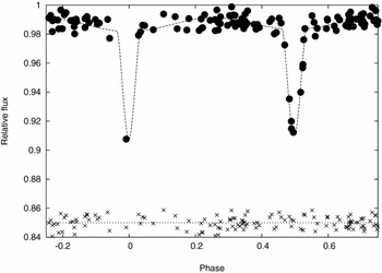
Figure 1. Hipparcos V photometry of η Mus and model fitting. The residuals, shifted by 0.85 on the flux axis, are shown below the curve fit.
The curve fit shown corresponds to the parameter set listed, with formal errors, in Table 1. Symbols have their conventional meanings and further details are given in the references of the preceding paragraph. This optimal fitting shows that an acceptable result can be found with inclination ~76°, but without significant third light, although the primary minimum is very poorly covered. Using the known colours and spectral types, a trial MS-like model can be made from two similar stars with total mass close to 7 M⊙. The period of 2.3963 d, together with Kepler’s third law and the provisionally adopted masses, yields a separation of about 14.4 R⊙. A corresponding typical MS pair would have undistorted mean radii of about 2.4 R⊙, implying relative radii r of around 0.17, not far from those found from the Hipparcos data analysis in Table 1. We adopt a mass ratio of unity in Table 1, anticipating the spectroscopic results discussed below, although the geometric parameters pertaining to the eclipse shapes are not significantly perturbed with the Hubrig et al. (Reference Hubrig, Le Mignant, North and Krautter2001) mass ratio. The lower secondary radius r 2 given in Table 1 does not directly reconcile with close similarity of the two stars, expected from the similarity of the two eclipse depths. The primary minimum is so poorly covered in the Hipparcos photometry, however, that it would be unwise to put weight on this initial fitting: it should be regarded rather as a guide.
Table 1. Initial curve-fitting results for the Hipparcos photometry of η Mus

2.2 Light curves of Hensberge et al
Starting from such preliminaries, ILOT type analysis was applied to the more extensive uvby photometry, kindly supplied by Dr H. Hensberge (Hensberge et al. Reference Hensberge2007; Figure 2). The essentially unity value of the spectroscopic mass ratio found below was used. There was fair agreement on the geometric parameters when determined separately (i.e. they were all within their probable errors), also with the Hipparcos light curve. We also found a small shift to the zero point of the phases (0.0040) calculated from the ephemeris of Hensberge et al. (Reference Hensberge2007). Bakış et al. (Reference Bakış, Bakış, Eker and Demircan2007) noted, from the high dispersion spectroscopy, a greater apparent rotation speed of the secondary than the primary (see also Section 3.1).
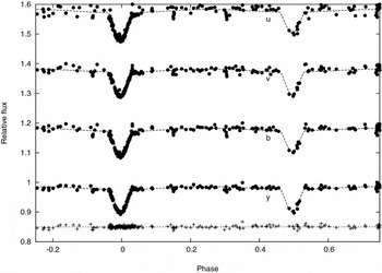
Figure 2. Light-curve fittings applied to the uvby photometry of η Mus, as presented by Hensberge et al. (Reference Hensberge2007). The relative fluxes are shown against phase with each curve vertically displaced by a linear displacement of 0.2. A greater primary depth in u is apparent, although the relative depths of the two minima are not so different at other wavelengths. No indication of a third light was found in this analysis. The residuals for the y fitting, shifted to 0.85, are shown at the bottom.
We then considered the possibility that the secondary is larger than the primary, and an occultation model for the primary eclipse proved to yield similar or slightly lower χ2 values to the fittings. Table 2 lists our finally adopted geometric parameters corresponding to an optimal modelling of the photometric data. An appreciable scale to the errors results from calculating them with proper account of parameter interdependence.Footnote 1 This reflects an inherent relatively low determinacy of curve fittings associated with these fairly shallow eclipses. Table 3 lists the magnitudes of either eclipsing star using the ubvy magnitudes of the main comparison (HD 114570) given by Hensberge et al. The secondary star is the more luminous in our model, but it can be seen that the primary becomes relatively brighter at shorter wavelengths, in keeping with a somewhat higher temperature. We discuss this point further in Sections 4 and 6. The relatively small proximity effects are evaluated as described in the curvefit manual of Rhodes (Reference Rhodes2008) corresponding to the assigned effective temperatures and uvby filter wavelengths.
Table 2. Summary results of fitting the light-curve data on η Mus from Hensberge et al. (Reference Hensberge2007) for the main geometric parameters

Table 3. Colour-dependent parameters in the η Mus close binary: luminosities of primary m 1 and secondary m 2 (in mag); linear limb-darkening u 1, u 2; gravity brightening τ1, τ2 and reflection effect coefficients E 1, E 2
The errors of these empirically determined component magnitudes m 1 and m 2 are estimated to be 0.02 mag. The other parameters are adopted from the theoretical work of van Hamme (Reference Van Hamme1993) (u), von Zeipel (Reference Zeipel1924) (τ), and Hosokawa (Reference Hosokawa1958) (E).
Hensberge et al. (Reference Hensberge2007) also referred to photometry during the interval 1983–1990, their analysis of which resulted in a refined period of 2.396320 d. We will discuss this in Section 5.
2.3 DSLR photometry
We have obtained more recent times of minima of η Mus using the developing technology of digital single lens reflex (DSLR) camera photometry (Blackford & Schrader Reference Blackford and Schrader2011). These developments come under the southern binaries monitoring program of the Variable Stars South (VSS) section of the Royal Astronomical Society of New Zealand (RASNZ). The data were gathered using an unmodified Canon 450D (Digital Rebel XSi) and Nikkor 180-mm lens operated at f4. Instrumental magnitudes obtained from differential aperture photometry, using four comparison stars, were corrected for atmospheric extinction and transformed to the standard system. We have stacked five minima observed in this way in Figure 3, where we also show optimal fits to the reduced B, V, and R data sets. One of the comparison stars was not in the frame for the first eclipse, and while this appeared to introduce a small shift of the out-of-eclipse reference flux, it does not disturb the shape or time of minimum. Keeping in mind the large number of individual measurements, the quality of the fits, as judged by the resulting reduced χ2 values, is quite comparable to those for the uvby data, and the corresponding geometrical parameters are essentially the same as those of Table 2, allowing confidence in the assigned error estimates.

Figure 3. Light-curve fittings applied to our BVR photometry of η Mus (see also Section 5.3). The R residuals are shown below, where the straight line at 0.85 guides the eye.
3 SPECTROSCOPY
Our spectroscopic data were taken with the High Efficiency and Resolution Canterbury University Large Échelle Spectrograph (HERCULES) of the Department of Physics and Astronomy, University of Canterbury (cf. Hearnshaw et al. Reference Hearnshaw, Barnes, Kershaw, Frost, Graham, Ritchie and Nankivell2002). This was used with the 1-m McLellan telescope at the Mt John University Observatory (MJUO; ~43°59′S, 174°27′E). Further information is given in Paper I (see also Skuljan, Ramm, & Hearnshaw Reference Skuljan, Ramm and Hearnshaw2004; Bakış et al. Reference Bakış, Bakış, Eker and Demircan2007; R. Idaczyk et al. in preparation). A 100-μm (slitless) optical fibre was used, enabling a resolution of approximately 41 000. A microlens in front of the fibre speeds up the focal ratio to an effective f/4.5 optical system, so that its 100-μm entrance pupil corresponds to about 4.3 arcsec on the sky. This accommodates the moderate-to-poor seeing conditions generally obtained. Average exposure times were about 200 s, which yield a signal-to-noise ratio (S/N) of ~100 in the selected spectral region (between ~470 and ~670 nm).
Some 50 separate exposures on η Mus were made on seven nights in the (southern) autumn of 2006, and most of these (43) were in the short interval May 17–20. These observations were made with a Spectral Instruments SITe series (1024 × 1024 pixels) camera. The camera only covers part of the whole spectral range, arranged to provide a region of good sensitivity. A further seven spectra were taken on August 19–20 and September 9 after the SITe camera had been replaced by an SI600s type. This camera has a larger number of smaller pixels (by a factor of ~0.60) to cover the whole field effectively in a 4096 × 4096 array. Two exposures of the visual companion (η Mus B) were included in this later period. Measurements based on these data from 2006 were first presented by Bakış et al. (Reference Bakış, Bakış, Eker and Demircan2007). Several more exposures of both η Mus A and B have been taken since 2010. We have independently examined all these data for the present paper. Although many of our results are very similar to those of Bakış et al. (Reference Bakış, Bakış, Eker and Demircan2007), there are some significant differences that will appear in what follows.
Initial data acquisition and reduction was performed with the on-site software package hrsp (Skuljan & Wright Reference Skuljan and Wright2007); however, the change of camera during the program entailed the use of different versions of hrsp. Version 4, used for much of the reductions presented here, allows results from the two camera formats to be easily compared, as well as being portable and robust.Footnote 2
The two-dimensional wavelength calibration in hrsp uses several hundred of the available Th/Ar reference lines (Skuljan et al. Reference Skuljan, Ramm and Hearnshaw2004). The static, highly controlled arrangement of HERCULES means that this calibration changes little from exposure to exposure (shifts up to tens of m s−1). Some further details about the performance of this spectrograph are given by R. Idaczyk et al. (in preparation).
hrsp stores processed data as ‘FITS’ files, which is convenient for further analysis using iraf (cf. Barnes Reference Barnes1993),Footnote 3 or other programs such as our spectrum module that we used in deriving RV values (see Section 3.2). Identifiable spectral lines for this close binary are given in Table 4, together with their central relative depths. The lines are similar to those listed for U Oph in Paper I, although corresponding to a slightly cooler spectral type. Unlike Paper II, where the relative effects of proximity and noise were large for V831 Cen, they are reduced in the case of η Mus. The two He i lines (6678 and 5875) were well placed for RV determinations, as also the Fe ii line at 5169. Two of the lines used by Bakış et al. (Reference Bakış, Bakış, Eker and Demircan2007) were found unsuitable for precise measurement. The Mg i 5173 line was seldom visible and the Fe ii 5018 line was often blended and distorted.
Table 4. Lines in the spectra (camera subfield 2) of η Mus used for RV determinations
The comments correspond to—ms: moderately strong; sd: strong but sometimes distorted; dmw: doublet moderately weak; wd: weak sometimes distorted; w: weak.
3.1 Rotational velocities
We fitted selected helium line profiles of η Mus at elongation phases using our computer program prof2. Results are shown in Figure 4 with parameters listed in Table 5.
Table 5. Profile fitting parameters for absorption lines
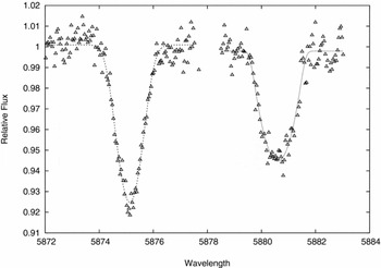
Figure 4. Results of profile fitting to the He i 5875 lines at elongation. The secondary is on the right.
Meanings of the parameters in Table 5 were explained in Paper I. For this particular pair of lines (from spectrum 34 in Table 6), the parameter r, measuring the mean projected rotational velocity, yields values of 42 ± 1 and 54 ± 2 km s−1 for primary and secondary components, respectively, after division by sin i. These values may be compared with those derived from corotation with the systemic rotation of 300 km s−1 and the fractional radii from Table 2. This would produce equatorial speeds of 45 ± 2 and 49 ± 3 km s−1, respectively, in the occultation primary photometric model of the system.
Table 6. Radial velocity data for η Mus (2006 May)

Although it is clear, both from these results and those of Bakış et al. (Reference Bakış, Bakış, Eker and Demircan2007), that the secondary rotates faster than the primary, this result is still not highly precise. The use of the iraf splot profile fitter on 65 line pairs produced a secondary/primary mean line width ratio of 1.31 ± 0.23, the error measure being associated with the appreciable scatter for many of the lines, whose maximum depths are still only a few percent of the continuum. The above fitting, for a relatively well-defined pair, confirms this result (ratio = 1.28 ± 0.10), although somewhat at variance with our photometric ratio (1.08 ± 0.08). The measured rotation speeds are, however, within their standard deviations of corotation. Asynchronous rotation of one or other star is still not outside the bounds of possibility, nor is the transit primary option for the photometric analysis. However, the secondary’s relatively high rotation is firmly evidenced, both by Bakış et al. (Reference Bakış, Bakış, Eker and Demircan2007) and ourselves. We must therefore give reasonable consideration to the possibility of a corotating, but enlarged, secondary star. Stars in an arrangement such as η Mus should normally synchronise within ~1 Myr (Vaz, Andersen, & Claret Reference Vaz, Andersen and Claret2007). We discuss this point further in Section 6.
3.2 Radial velocities
The RV measurements involved only strong lines, as listed in Table 4. If more than one line was present in an order, only the most clearly defined one was used. Our Python module spectrum, written to speed up the process of RV determination from line shifts, uses the open source SciPy library’s optimize subpackage and its least-squares module curve_fit to fit a rotation-broadened profile to the selected spectral lines. Typically ~10 lines spread across the available spectral range were initially selected. Manual identification of useful lines is first carried out with the aid of iraf’s splot command. High S/N lines with good visibility that lack significant telluric contamination are favoured. It can be deduced from Figure 4 that for orbital phases within about ±0.03 of 0.0 or 0.5 lines from the components will overlap to some extent. Three or four exposures among the 43 listed in Table 6 are thus affected. Although all the listed observations are shown in Figure 6, the inclusion of these near-conjunction points in the fitting does not alter the resultant parameter specifications by more than their probable errors. Reference wavelengths of the selected lines were taken from the ILLSS website.Footnote 4 As spectrum runs, selected images are displayed together with a profile fitting. Barycentric velocities are calculated, examined, stored, and averaged over (usually nine) lines.
The 2006 May schedule of timings, heliocentric corrected RV (RV1, and RV2) and systemic RV (γ) measures are given in Table 6. The errors of mean line centre positions in Table 6, typically ~2.0 km s−1, are estimated, from internal agreements of the separate measures.
The longer wavelength lines can be affected by telluric intrusions that can vary in strength from exposure to exposure. Visual inspection is then useful, taking into account S/Ns, and RV measures derived from spectrum were checked against eye-based measurements.
The RVs were also checked by inter-correlating selected spectral regions. A result is shown in Figure 5. It is of interest to compare this diagram with results obtained from the procedures mentioned above. It seems clear that spectral irregularities or window positioning affect any cross-correlation function (ccf) symmetry that might apply to an idealised case. These irregularities extend to the peak and influence its location at the level of several km s−1. Such effects can be noticed in Figure 1 of Bakış et al. (Reference Bakış, Bakış, Eker and Demircan2007) (see also Rucinski Reference Rucinski2002).

Figure 5. Cross-correlation of the two He i 6678 lines corresponding to image 38 in Table 6. The abscissae are in km s−1, while ordinates are normalised to unity at perfect correspondence and scaled so that the average deflection in a window is zero. This will entail some anti-correlation as the two line absorption peaks move apart. The two equal window locations have a velocity separation of 206.2 km s−1, so the net displacement of the two lines indicated by the ccf peak shift of 10.2 km s−1 is 216.4 km s−1, which may be compared with 222.3 km s−1 from the measures in Table 6. The ccf reflects line asymmetries, particularly of the secondary, whose lines tend to show less slope on the primary-facing side. High-frequency noise also affects the peak region. It is true that readjustment of the correlation windowing after a preliminary result as shown here can result in a closer agreement with the RVs of Table 6; however, the diagram shows that cross-correlation procedures to derive good RVs are not necessarily straightforward (cf. Rucinski Reference Rucinski2002).
We used the same model for fitting the RV variations (fitrv4a) as in Papers I and II. Proximity effects such as reflection and non-spherical stellar distortions are not significant for the present case, although the fitting program automatically includes them. Results are shown in Figure 6 and corresponding parameters given in Table 7. Although the close binary must have some level of dynamical interaction with its companion stars, perturbations to the close orbit are small, and, keeping in mind the findings of Zahn (Reference Zahn1977), a priori neglect of any eccentricity in the analysis is reasonable.
Table 7. Adopted absolute parameters for the η Mus A close binary. Formal errors are shown in parentheses to the right and relate to the least significant digits in the corresponding parameter values


Figure 6. Measured RVs are plotted against a fitting function that takes into account both proximity and eclipse effects. The primary (higher Te ) star approaches (more negative RVs relative to the centre of mass) after phase zero. The inclination is sufficiently low as to render the Rossiter–McLaughlin effect insensible.
4 ABSOLUTE PARAMETERS
The RV solutions shown in Figure 6 correspond to the K 1,2 amplitudes given in Table 7. The two amplitudes are essentially equal to within their measurement accuracy, although the two spectra are distinctly different as seen in Figure 4. The orbital semimajor axis is derived given the adopted inclination (76.°5). Kepler’s law then allows the shown masses to be obtained. The radii come from multiplying the orbit’s radius by the fractional radii given in Table 2. The velocity of the centre of mass V γ corresponds to the adopted epoch for those few days in 2006 May (JD2453874.2708) whose data were used for the RV curve fittings. The masses and radii of Table 7 are in reasonable agreement with the B8V spectral types and corresponding effective temperatures given in Section 1, according to Table 3.6 in Budding & Demircan (Reference Budding and Demircan2007), while the slightly shallower secondary minima (at shorter wavelengths) go with its temperature decrement. This is in agreement with the luminosity and radius ratios derived from Table 7.
With the Hipparcos parallax, the absolute V magnitudes are 0.21 and −0.08 for the primary and secondary, respectively. According to their masses and recent Padova modelling data (Bressan et al. Reference Bressan, Marigo, Girardi, Salasnich, Dal Cero, Rubele and Nanni2012), both stars are within reasonable errors of determination to the zero-age main sequence (ZAMS). If we adopt the higher temperature of Hubrig et al. (Reference Hubrig, Le Mignant, North and Krautter2001) to derive the photometric parallax from the formula
 \begin{equation}
\log \Pi = 7.454 - \log R -0.2 V - 2 F_V^{\prime },
\end{equation}
\begin{equation}
\log \Pi = 7.454 - \log R -0.2 V - 2 F_V^{\prime },
\end{equation}
5 OTHER COMPONENTS
5.1 η Mus B
The chemical peculiarity of η Mus B was mentioned in the Introduction. We present in Table 8 a listing of lines, mostly identified from the ILLSS and NIST catalogues (Coluzzi Reference Coluzzi1993, Reference Coluzzi1999; Ralchenko et al. Reference Ralchenko, Kramida and Olsen2011), as well as a few still unidentified features. The wavelengths given in Table 8 correspond to a predetermined Doppler shift of 14.5 km s−1; however, the mean shift of the 479 lines is non-zero, implying a better estimate for the mean RV of η Mus B is 14.3 km s−2. The difference between this value and the γ velocity of the close binary in 2006 was used by Bakış et al. (Reference Bakış, Bakış, Eker and Demircan2007) as an argument for the unbound condition of the wide system η Mus AB; however, Butland & Budding (Reference Butland and Budding2011) showed that this γ velocity varies. The mean γ velocity turns out to be measurably the same as that of η Mus B, so we can attach more confidence to Tokovinin’s (Reference Tokovinin1997) appraisal of the wide system.
Table 8. Spectrum measures for η Mus B

The measured wavelengths are shown with an ad hoc correction of 14.5 km s−1 to give closeness to the (air) reference values. The differences between these two (Δλ) are listed in the fourth column. Equivalent widths (EW) are given in units of mÅ of the local continuum. The fifth column identifies the expected source atom or ion, usually on the basis of wavelength proximity. The remarks correspond to—b: a blend, often with an expected close feature named; sometimes not, in the case of various possibilities; id: uncertainty of identification; cs: a well-known feature of cool stellar spectra, or cgs: associated more with a low gravity cool atmosphere; hs: a feature expected in normal dwarf stellar spectra of type earlier than A4. The data from which this table was composed can be made available to any interested specialist.
We examined a number of lines to assess the rotation of η Mus B, as in Section 3.1 for the close binary. Six clearly defined and symmetric lines selected for profile fittings were Fe ii 6456, Si ii 6371, Co i 5984, Fe i 4957, Mg i 4703, and Fe i 4525. The average projected equatorial rotation speed was found to be 31.7 ± 1.8. The convolved Gaussian component of the full line broadening was 22.5 ± 2.0.
5.2 η Mus C
If this star is bound to the bright close binary, as would seem likely given the bound nature of the much wider AB system, it must have orbital period in the order of 3000 yr. Although Hubrig et al. (Reference Hubrig, Le Mignant, North and Krautter2001) reported ~10 mag (J), it was not resolved by ‘lucky imaging’ techniques in the V range (Idaczyk Reference Idaczyk2012).
5.3 η Mus D
A slight difference between the γ velocity applying to the RVs of 2006 May and September was noticed when the present authors re-analysed the spectra, and this prompted further observations since 2010. It became clear that the γ velocity of the main pair cycles on a relatively short timescale (~5 yr), as shown in Figure 7.
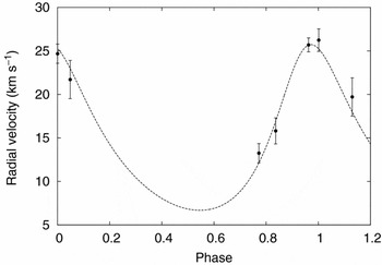
Figure 7. Preliminary orbital model fitting to observed variations of the γ velocity of η Mus.
The variations of γ velocity suggest observable effects in the time of minima, prompting further photometry. The model corresponding to Figures 7 and 8 yields a mass function of about 0.142. This would correspond to a third mass about 2.3 solar masses if the orbit were roughly coplanar with the central close pair. In turn, this would correspond to an A-type star about a couple of magnitudes fainter than either of the close binary stars, or about 6% of the system light. Such a third light contribution was considered in Section 2, but not identified. Since all the measured lines are associated with the B-type stars of the close pair, it seems unlikely that this new component would interfere with the RV model presented in Section 3, but this point should be examined further as the model for this wider orbit becomes better known.

Figure 8. Measured O − C from times of minima of η Mus A due to η Mus D. The calculated light travel time derived from the γ velocity fitting in Figure 7 is also shown.
5.4 Time of minimum variations
H. Hensberge (private communication, 2011) kindly forwarded the data they used to refine the mean orbital period of the close binary. These data are from patrol-type observations not specific to η Mus and so rather discontinuous. Here and there, the material becomes more bunched, however, and may include observations within eclipse minima. We sought to fit such data groups for timing variations, although derived shifts cannot have the same reliability as for completely covered eclipses.
We considered six main groups of data over the interval 1983–90, containing around a dozen points each. A set of 33 observations with greater scatter from early 1975 also sent by Dr Hensberge make up seven sparse light curves. In testing these data sets, we assumed the light curve model corresponding to the parameters of Table 2 and allowed only the zero point of the phases (Δφ0) and system luminosity (‘unit of light’) to vary. The scale of O − C differences found was generally consistent with their expected range (~0.01 d), but with an appreciable scatter. Unfortunately, these findings were too few and from essentially too small data sets to be convincing.
On the other hand, more consistency has been found between the spectrometry-derived third orbit and recent determinations of times of minima from full eclipse coverage using DSLR techniques. Preliminary findings were reported by Idaczyk (Reference Idaczyk2012) and are shown in Table 9 and Figure 8, where we include points from Bakış et al. (Reference Bakış, Bakış, Eker and Demircan2007), as well as our own observations. A fuller tally of results will be published in due course.
Table 9. O − C data for η Mus

6 DISCUSSION
The RV amplitudes and masses given in Table 7 are not significantly different from those given by Bakış et al. (Reference Bakış, Bakış, Eker and Demircan2007). There are, however, at least two major differences of interpretation between Bakış et al. (Reference Bakış, Bakış, Eker and Demircan2007) and the present study. We dealt already with one of these in Section 5, namely that the visual companion η Mus B does have a real physical connection to the close binary, even though their mean RVs may sometimes appear different by several times greater than the error of the determination. Bakış et al. confirmed the likely membership of η Mus B to the LCC concentration of the Sco–Cen OB2 association, though their argument cast doubt on that of η Mus A. The inner A–D orbit now supports the inference of a common origin for the multiple star.
The other difference arises from the confirmed result that the secondary has a higher projected rotation speed than the primary. Our findings support those of Bakış et al. (Reference Bakış, Bakış, Eker and Demircan2007), although we claim this result does not have a very high precision. Our use of the iraf profile fitter on 65 line pairs produced an appreciable scatter in widths for many of the lines, but we should note that maximum depths are still only a few percent of the continuum. Our adopted results in Table 7 give that the secondary star is larger than the primary, though it must be cooler to account for the difference in depths of the two eclipses. At the same time, the masses of the two stars are essentially the same to within measurement errors. As with Bakış et al. (Reference Bakış, Bakış, Eker and Demircan2007), we assign a slightly smaller mass to the secondary star. Keeping in mind the normal relation of mass and radius for MS stars, how then does it come to be larger?
Our interpretation of this point is based on models of very young stars, still in the process of arrival at the ZAMS (Siess, Dufour, & Forestini Reference Siess, Dufour and Forestini2000). The irregular episodes of enhanced luminosity during the final descent to the ZAMS are sometimes associated with the ‘deuterium flash’, though the word flash may be somewhat misleading for time intervals of several hundreds of thousands of years. Recent tabulated data from the CMD webpage (Bressan et al. Reference Bressan, Marigo, Girardi, Salasnich, Dal Cero, Rubele and Nanni2012) used to make isochrones can be easily adapted to show radius versus time, since luminosities and effective temperatures are listed for given masses over specifiable age ranges, including PMS stages. The final condensation to the MS stage seen at the left of Figure 9 shows that there can be an appreciable interval of time (of the order of a few ×0.1 Myr) during which a less massive star would be significantly larger than the more massive one.

Figure 9. The evolution of stellar radii (solar units) derived from the data of Bressan et al. (Reference Bressan, Marigo, Girardi, Salasnich, Dal Cero, Rubele and Nanni2012) for stars of 3.0–3.6 solar masses, as indicated. Component radii can be seen to grow appreciably larger than those of Table 7 before the relatively rapid expansion away from the MS at the right.
An alternative scenario in which the putative secondary is slightly more massive than its partner could be thought of. The difference in its radius might then be associated with a pair of similar stars approaching the end of their MS stage. At some point, the relatively rapid growth of the more massive star could then allow for the obtained ratio of radii to be realised. However, checks of stellar evolution tracks for stars of mass around 3.3 M⊙ (Figure 9 and Bertelli et al. Reference Bertelli, Nasi, Girardi and Marigo2009) show that by the time this might occur, given the very small mass differential, both stars would have to become significantly larger than the radii given in Table 7.
Overall, our picture of the η Mus multiple star, in not requiring a recent close encounter with an unidentified passing object, appears simpler and more direct than the account of Bakış et al. (Reference Bakış, Bakış, Eker and Demircan2007), but a number of intriguing points remain. How did this very young stellar system arrive in the configuration found? The inferred young age contrasts with the Sartori, Lépine, & Dias (Reference Sartori, Lépine and Dias2003) 16–20 Myr age for stars selected from the Sco–Cen OB association, although characterising all the stars in this very large association by a narrow range can be questioned while ongoing star formation has been identified within it (Preibisch & Mamajek Reference Preibisch, Mamajek and Reipurth2008). Paper II’s study of the comparable system V831 Cen produced an age within the range of Sartori et al. (Reference Sartori, Lépine and Dias2003), but essentially the same procedures have led to the much younger result for η Mus. We can also ask about the Ap nature of η Mus B, noting also the similar condition of the third star in the comparable system V831 Cen. All such questions, as well as the atypical binary configuration, call for continued observations of the intriguing η Mus multiple star.
7 CONCLUSIONS
The Sco–Cen complex is an important astrophysical laboratory for studies of recently formed stars. Close binary or multiple systems, especially if eclipses are present, represent a small but highly significant subgroup within this population, whereby hard evidence on stellar masses, luminosities, and composition can be quantified. It is also important that such evidence continues to be gathered, carefully checked and, where possible, counterchecked by alternative groups, methods, and technologies.
Our challenge to inferences about the complete system previously made by Bakış et al. (Reference Bakış, Bakış, Eker and Demircan2007) are underpinned, to a large extent, by our finding that η Mus B is gravitationally bound to the close binary. This relates to the recent discovery of η Mus D, and our new photometric and spectroscopic data about this.
Our absolute parameters, especially the stellar radii, argue for a young age, i.e. that the secondary of η Mus A is still condensing to the MS, so that its unexpectedly high rotation speed is due to its greater size; and that neither it nor the primary is asynchronously rotating, but their rotation speeds are consistent with tidal locking. These claims invite still more detailed observational checks and future research. η Mus thus appears a special case to test stellar modelling theory, given the precise age determination we infer.
ACKNOWLEDGEMENTS
We acknowledge useful input from Professors O. Demircan and A. Erdem as well as research students and staff of the Department of Physics, 18th March University of Çanakkale, Turkey. Many of the original set of spectrograms studied in this paper were gathered by V. Bakış and H. Bakış during the period of study in New Zealand in 2006 that was supported by the Science Research Council of Turkey (TÜBİTAK).
Generous allocations of time on the 1-m McLennnan Telescope and the HERCULES spectrograph at the Mt John University Observatory supporting the Southern Binaries Programme have been made available through its TAC and Director, Dr K. Pollard, and previous Director, Prof J. B. Hearnshaw. Useful assistance was provided by the MJUO management (A. Gilmore and P. Kilmartin). Considerable help with the use and development of the hrsp software (leading up to the latest version 5) was given by its author Dr J. Skuljan. Besides hrsp, the user-friendly freeware imagej was found useful for preliminary image checks. We are also grateful to Matthew Davie of UoC’s Department of Physics and Astronomy for new spectroscopic data on η Mus.
Encouragement and support for this program has been shown by the Carter Observatory and the School of Chemical and Physical Sciences of the Victoria University of Wellington, as well as the Royal Astronomical Society of New Zealand and its Variable Stars South section (http://www.variablestarssouth.org). We thank VSS Director Tom Richards for advocating DSLR photometry in support of this program.


