


1 INTRODUCTION
During the Last Glacial Maximum (~26.5 to 19 ka B.P., Clark and others, Reference Clark2009) the Antarctic Ice Sheet in most regions extended all the way to the continental shelf (Anderson and others, Reference Anderson, Shipp, Lowe, Wellner and Mosola2002; Bentley and others, Reference Bentley2014), but details of the deglaciation history are poorly known. Especially, knowledge of the glacio-geological history of Dronning Maud Land (DML), East Antarctica, is very sparse even during the Holocene period (Mackintosh and others, Reference Mackintosh2014). For this period, such knowledge is required to better constrain ice-sheet models, particularly, models used to make reliable predictions on ice-sheet behaviour under possible warming scenarios (e.g., DeConto and Pollard, Reference DeConto and Pollard2016). To gain such knowledge, we have several sources; namely, marine geological records provide information on past ice-sheet extent (Elverhøi, Reference Elverhøi1981; Kristoffersen and others, Reference Kristoffersen, Strand, Vorren, Harwood and Webb2000; Hillenbrand and others, Reference Hillenbrand2014) and exposed rocks at nunataks provide past ice-sheet elevation constraints (e.g., Ingólfsson and others, Reference Ingólfsson1998; Mackintosh and others, Reference Mackintosh2014; Suganuma and others, Reference Suganuma, Miura, Zondervan and Okuno2014). In addition, ice rises can provide local, high-resolution information of the Holocene history near ice shelves (Hindmarsh, Reference Hindmarsh1996; Conway and others, Reference Conway, Hall, Denton, Gades and Waddington1999; Nereson and Waddington, Reference Nereson and Waddington2002; Martín and others, Reference Martín, Hindmarsh and Navarro2006, Reference Martín, Gudmundsson, Pritchard and Gagliardini2009a; Drews and others, Reference Drews, Martín, Steinhage and Eisen2013, Reference Drews2015; Kingslake and others, Reference Kingslake, Martín, Arthern, Corr and King2016).
Ice rises exhibit their own local flow that differs from the surrounding ice-shelf flow. Like a miniature ice sheet, the flow originates from the summit and flows down towards the flanks (Matsuoka and others, Reference Matsuoka2015). The information regarding this ice flow is recorded within the ice as distinct stratigraphic features such as Raymond arches (Raymond, Reference Raymond1983). Consequently, ice flow models have been used to interpret these features in ice stratigraphy and retrieve information such as mass balance (Drews and others, Reference Drews, Martín, Steinhage and Eisen2013, Reference Drews2015), divide migration (Nereson and others, Reference Nereson, Raymond, Waddington and Jacobel1998) and the surrounding ice flow characteristics (Martín and others, Reference Martín, Hindmarsh and Navarro2006, Reference Martín, Gudmundsson and King2014). The main challenge in this technique is accounting for the complexities of the ice flow near the flow divide (within 2–3 times the icethickness from the summit) while determining past changes in the surrounding cryosphere. Recently, Kingslake and others (Reference Kingslake2014) obtained direct observations of englacial velocities, confirming that no isotropic Glen-flow approximation could approximate the complexity of the ice flow in this region. Our approach here is to focus on areas slightly away from the summit (where the horizontal advection is very low), giving greater confidence that the ice is approximately isotropic (e.g., Martín and Gudmundsson, Reference Martín and Gudmundsson2012).
In this study, we use an ice flow model to decipher the evolution of Blåskimen Island, an ice rise between the Fimbul and Jelbart Ice Shelves in Western DML (Fig. 1). Goel and others (Reference Goel, Brown and Matsuoka2017) found that this ice rise is currently thickening, and also that the present summit has been stable for at least the past ~600 years. We test several hypotheses to elucidate the onset of recent thickening and past changes in surface mass balance (SMB).
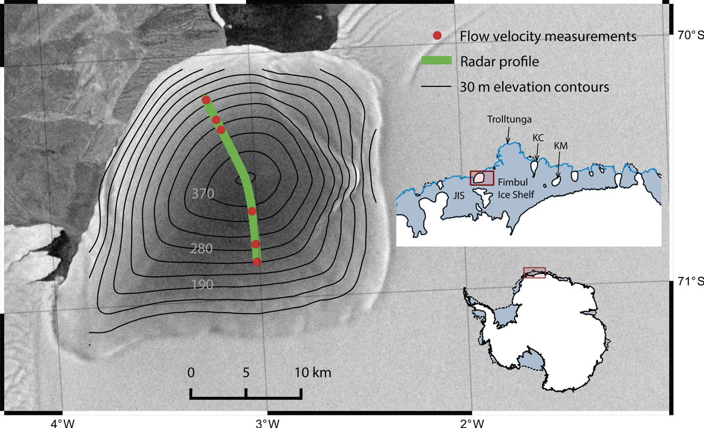
Fig. 1. Blåskimen Island ice rise, western Dronning Maud Land. Ice-surface topography is shown with contours at 30 m intervals (Goel and others, Reference Goel, Brown and Matsuoka2017). Green curve marks the radar profile. Red dots are positions of GPS stakes used to measure flow velocity. Insets show the coverage of the map, indicating Jelbart Ice Shelf (JIS) and two adjacent ice rises where ice cores were drilled: Kupol Moskovskij (KM) and Kupol Ciolkovskogo (KC). The background image is Radarsat-1 satellite imagery (Jezek and others, Reference Jezek2002).
2 STUDY AREA, DATA AND METHODS
2.1 Blåskimen Island
Blåskimen Island is an isle-type ice rise located at the calving front between the Fimbul and Jelbart Ice Shelves (Fig. 1). Goel and others (Reference Goel, Brown and Matsuoka2017) made shallow and deep radar sounding, GPS measurements of surface ice flow, a shallow firn coring and temperature measurements at the summit. The firn core was dated back to 1996 primarily using its oxygen isotope ratios (Vega and others, Reference Vega2016). These data were used to estimate the recent mass balance of Blåskimen Island using the input–output method (Goel and others, Reference Goel, Brown and Matsuoka2017). Before we describe the data used to constrain our flow model in the next section, we summarize here the glaciological settings of Blåskimen Island.
Blåskimen Island is one of the larger isle-type ice rises (area: 651 km2). This ice rise is largely dome-shaped, with a pronounced ridge extending to the south-west from its summit 410 m a.s.l and 350 m above the adjacent ice shelf. The bed is largely flat beneath the summit and slopes towards the south, with a mean elevation of 110 m below sea level (Fig. 2b). The firn temperature is nearly uniform at −16 °C between 8 and 12 m depths, and no major melt features were found in the firn core. The SMB at the summit is 0.76 m ice equivalent per year (mieq a−1), between 1996 and 2013 (20 m-long firn core; Vega and others, Reference Vega2016). Reflectors visible through shallow-sounding radar show that the spatial pattern in SMB remained the same at least for the last decade. SMB estimates obtained by dating these radar reflectors show higher SMB on the upwind south-east slope than that on the downwind north-west slope by ~37% (Fig. 2a). This pattern is likely a result of interaction of northeasterly precipitation from storms and the prevalent southeasterly katabatic winds with the ice rise topography. Surface ice flow is slightly asymmetric; the southern slope flows faster than the northern slope, but the flow speed is <15 m a−1 (Fig. 3). Using these data with the input–output method, it was found that the ice rise has been thickening at ~0.12–0.37 m a−1 over the last decade.
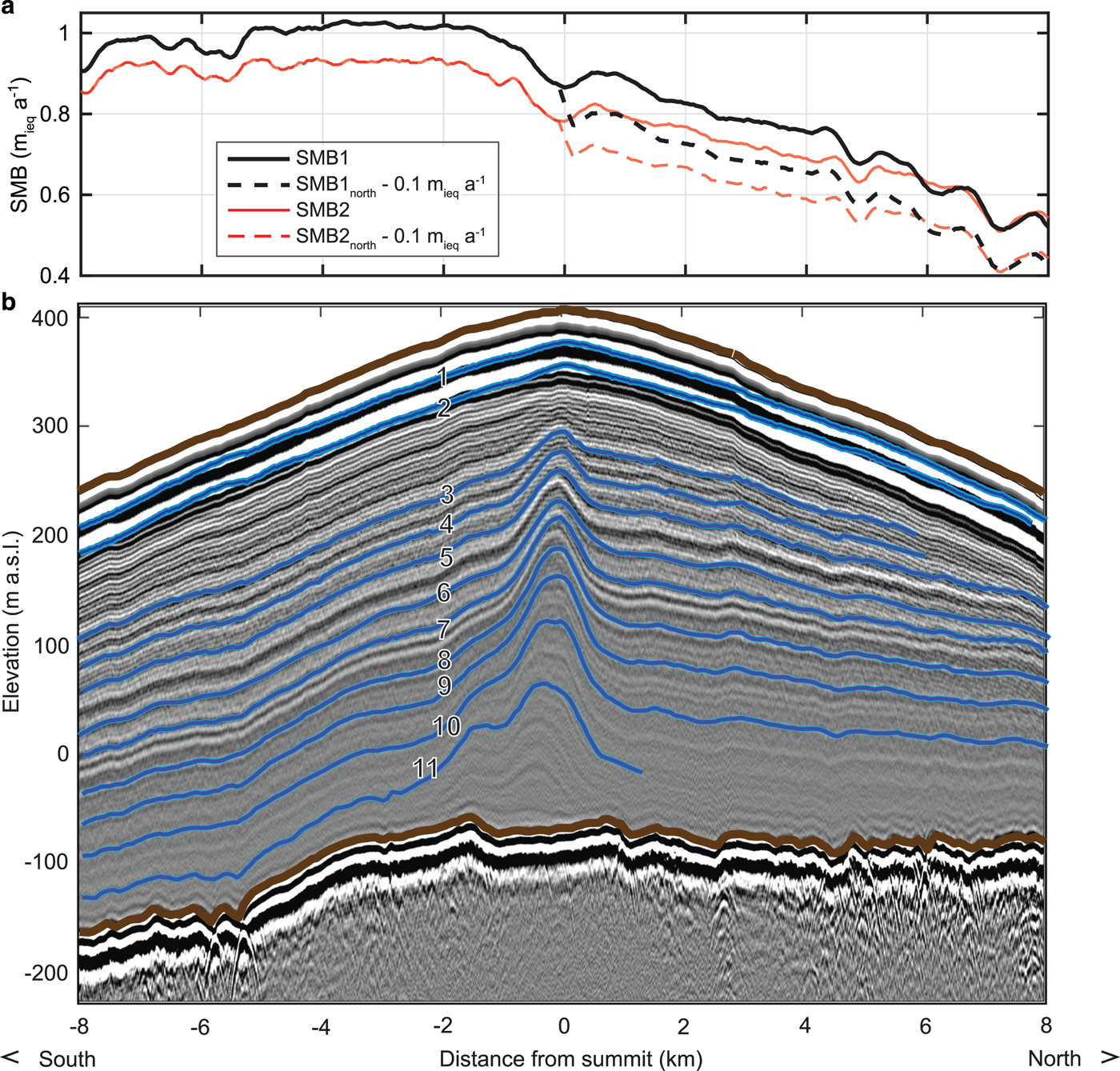
Fig. 2. Cross-section of the ice rise along the radar profile from Figure 1. (a) Radar and firn core derived surface mass balance (SMB) used as an input to the model (Goel and others, Reference Goel, Brown and Matsuoka2017). Black curve shows the SMB estimate derived assuming only vertical variability in density (SMB1); red curve accounts for both vertical and lateral variability in density (SMB2). Dashed curves show potential SMB in the past (ΔSMBnorth = –0.1 mieq a−1). (b) Selected reflectors (blue) in the 2-MHz radargram (3–11). Reflectors 1 and 2 were instead imaged using 400-MHz shallow-sounding radar and superimposed. Thick brown curves mark the ice rise surface and bed.
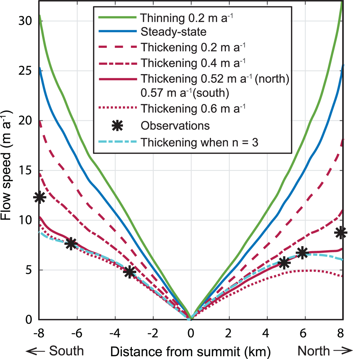
Fig. 3. Modelled and observed surface ice flow speeds. Curves show the different modelling experiments. Markers show observations. The solid red curve used a thickening rate of 0.52 mieq a−1 in the northern flank and 0.57 mieq a−1 in the southern flank. The dotted blue curve used a different rheology with n = 3 and thickening rate of 0.54 mieq a−1 in the northern flank and 0.61 mieq a−1 in the southern flank.
Deeper radar reflectors show upward arches beneath the current summit known as Raymond arches (Fig 2b). These arches are formed due to accumulated effects of variable vertical strain near the ice divide and require stable conditions to form. Vertical alignment of the arches and the characteristic times suggested by Martín and others (Reference Martín, Gudmundsson, Pritchard and Gagliardini2009a) show that the summit position has been stable within several kilometres at least in the past 600 years but no longer than several millennia.
2.2 Data
We modelled a radar profile (both deep and shallow radar data available along this profile) that passes through the ice-rise summit (Figs. 1, 2). The selected radar profile is 16 km long and aligns north–south, marked 2–2’ in Figure 1b of Goel and others, (Reference Goel, Brown and Matsuoka2017). Along the modelled profile, the ice thickness varies between 312 and 476 m, with the bed nearly flat north of the summit and sloping down towards the south (Fig. 2b). The flow-speed varies from negligible near the summit to 13 m a−1 in the flanks. As this profile aligns with the steepest descent path on the surface, the ice flows mostly along the profile on both sides of the summit. Of all four profiles through the ice-rise summit from a previous study (Goel and others, Reference Goel, Brown and Matsuoka2017), the profile modelled here has the smallest flow divergence. Along this profile, the measured surface across-profile strain rates are 3–8% of the vertical/along-profile strain rates, and across-profile strain rates are slightly larger in the northern flank. However, this asymmetry in divergence is smaller than the asymmetry in vertical strain-rates between the north and the south due to differences in SMB (~40%). Thus, the strong north–south asymmetry in the stratigraphy should primarily be a consequence of asymmetry in the SMB, not the flow divergence.
We tracked nine radar reflectors in the deep-sounding (2 MHz) radargram covering the depths from 126 to 386 m below the ice surface. We also tracked two reflectors from the shallow-sounding (400 MHz) radargram within the shallowest 50 m. Among these 11 reflectors, eight reflectors are tracked for the entire model domain to evaluate the model experiments. As it is illustrated in Figure 2, these eight reflectors are representative of the entire radio stratigraphy of the ice rise. We examined sets of conditions with which the ice flow model gives the best match between the modelled isochrones and these radar reflectors.
2.3 Ice flow model
We used a thermo-mechanical full-Stokes ice flow model based on the Elmer/Ice suite (Gagliardini and others, Reference Gagliardini2013). The initial and boundary conditions of the model, as well as the rheology, were adapted from Martín and others (Reference Martín, Hindmarsh and Navarro2009b). We describe the model briefly here and refer the reader to these papers for further details.
For the ice flow, we assume plane-strain 2D flow along the profile with no basal sliding and a stress-free upper surface. At the numerical domain margins, we prescribe the velocity variation with depth to follow theoretical isotropic-laminar flow under the shallow-ice approximation (e.g. van der Veen, Reference Van der Veen1999, Section 4.2). For steady state, the ice flow flux through these margins is prescribed to balance the total input SMB. To simulate thickening/thinning for a given input SMB, the ice flow flux at the margins is adjusted as per the desired mass balance. For the thermal conditions, we assume a constant, uniform geothermal flux of 60 mW m−2 (Fox Maule and others, Reference Fox Maule, Purucker, Olsen and Mosegaard2005), and a uniform surface temperature of −16.2°C (measured at 10 m depth in the borehole at the summit, Goel and others, Reference Goel, Brown and Matsuoka2017). The bed is assumed nondeformable and thus no heat advection occurs through the bed. At the downstream domain margins, we assume a null horizontal gradient of temperature. The model is thermo-mechanically coupled such that the flow-law parameter is updated at each time step according to a new ice temperature field (Eqn (13) in Martín and others, Reference Martín, Hindmarsh and Navarro2009b which is based on Dahl-Jensen., Reference Dahl-Jensen1989) determined by solving the heat equation that considers heat advection, diffusion and strain heating (see details in Martín and others, Reference Martín, Hindmarsh and Navarro2009b).
Regarding the rheology, we use Glen´s flow law with two values of the rheological power index n. One value is the widely used value of n = 3 (e.g., Cuffey and Paterson, Reference Cuffey and Paterson2010), the other is n = 4.5, which was used to describe the ice rheology measured at the Greenland Summit (Gillet-Chaulet and others, Reference Gillet-Chaulet, Hindmarsh, Corr, King and Jenkins2011). For both cases, we determined the enhancement factor E by tuning its value so that the modelled ice rise surface matches well with the observed one. We used the surface elevations, not flow speeds, because a large number of surface elevation observations makes it easier to constrain the enhancement factor as compared with flow speed. However, we exclude the surface topography in the divided region where the model does not adequately describe the ice rheology and also near the downstream boundary of the model. The latter is excluded in other studies as well, as the error induced by imposing boundary conditions at the vertical margins can then propagate into the solution domain as far as a few times the ice thickness from the downstream boundary (Hvidberg, Reference Hvidberg1996; Martín and others, Reference Martín, Hindmarsh and Navarro2009b). For n = 3, we use an enhancement factor E = 4, whereas for n = 4.5 we use E = 1.5 × 10⁻⁷ Pa−1.5. Both E values are typical for their case and the change in units accounts for the higher Glen's flow law exponent. In the next section, we present the results from experiments with n = 4.5 and compare with those with n = 3 in Section 4.
3 RESULTS
3.1 Recent mass balance
The first model run assumes steady state. We apply mass-conserving boundary conditions at the model flanks so that the ice rise is in balance when the present-day SMB is applied. We initialize the model with the present-day surface topography but allow the ice surface to evolve. The model is run for 40 times of the characteristic time T (=SMB/ice thickness = 625 years), which is ~25 000 years. After this time, further iterations do not change the isochrone pattern. The resulting ice temperatures at the ice-rise base were well below freezing, having a maximum temperature of −9.2°C, indicating no basal melting. At the surface, we find that the modelled surface flow speeds increase away from the summit on both flanks (Fig. 3). However, these modelled flow speeds are twice those of observations, indicating that the ice rise is not in steady state.
Next, we tested the more likely hypothesis of a thickening ice rise in the model, as the field data show a thickening in the last decade. Along the modelled radar profile, the observed thickening rates are less than the ice-rise mean thickening rate, ranging within 0.16–0.30 mieq a−1 (a flowline setup along the flowlines FA and CD; Goel and others, Reference Goel, Brown and Matsuoka2017). For this experiment, we initialize the model with the present-day ice-surface topography, but its elevation is everywhere lower by dH (i.e. ice is uniformly thinner than the present-day value by dH). The downstream outgoing ice flux is adjusted to maintain the ice rise in balance for the present-day SMB. After the model run is for 25ka, the model reaches a steady state, which becomes the initial condition of a thickening experiment. The ice-thickness/elevation difference dH is set so that the ice rise reaches the present-day thickness/elevation after the thickening period. We examined thickening for a period of 40 years but at two thickening rates: 0.4 mieq a−1 (dH = 40 × 0.4 = 16 m) and (ii) 0.6 mieq a−1 (dH = 24 m). The downstream outgoing ice flux is lowered to thicken the ice rise at each prescribed rate.
Consider now the modelled flow speeds after the 40-year thickening period. Experiment (i) in Figure 3 gives flow speeds larger than the observed values, whereas experiment (ii) gives values lower than the observed values, but with a relatively good match on the southern flank. This match motivated experiment (iii), in which we input the differential thickening rates of 0.52 mieq a−1 for the northern flank and 0.57 mieq a−1 for the southern flank. As shown in Figure 3, this experiment best reproduces the observed flow speed overall, but not in the vicinity of the downstream flow margin. This is a known artefact in our boundary conditions (Hvidberg, Reference Hvidberg1996). For completeness, we also ran a thinning experiment with a thicker initial steady state by 16 m, which was later thinned at a rate of 0.2 mieq a−1 for 40 years. As expected, after the 40-year thinning period, the resultant surface flow speeds are even faster than the steady-state case. Therefore, we conclude that a thickening ice rise best reproduces the flow-speed observations along this profile.
3.2 Onset of thickening
To determine when the present thickening started, we cannot use the observed flow-speed distribution because the ice flow speeds respond instantaneously to the ice thickness. So instead, we model englacial isochrones for a thickening ice rise over different periods in the past and compare them with the observed radar reflectors (Fig. 4).
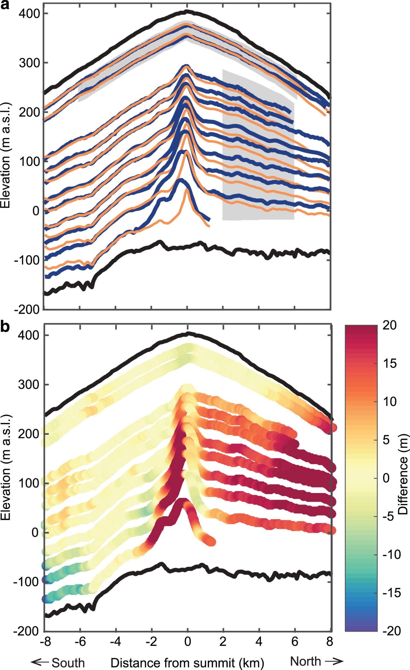
Fig. 4. Isochronous stratigraphy for the experiment with thickening of 0.52 mieq a−1 on the northern flank and 0.57 mieq a−1 on the southern flank for 40 years. (a) Modelled isochrones (orange) shown with observed reflectors (blue). Grey region behind the shallowest two reflectors was used to calculate MAD in Figure 5. (b) Elevation difference D between the radar reflectors and the corresponding modelled isochrones (Eqn (1)). Black curves mark upper and lower ice surfaces.
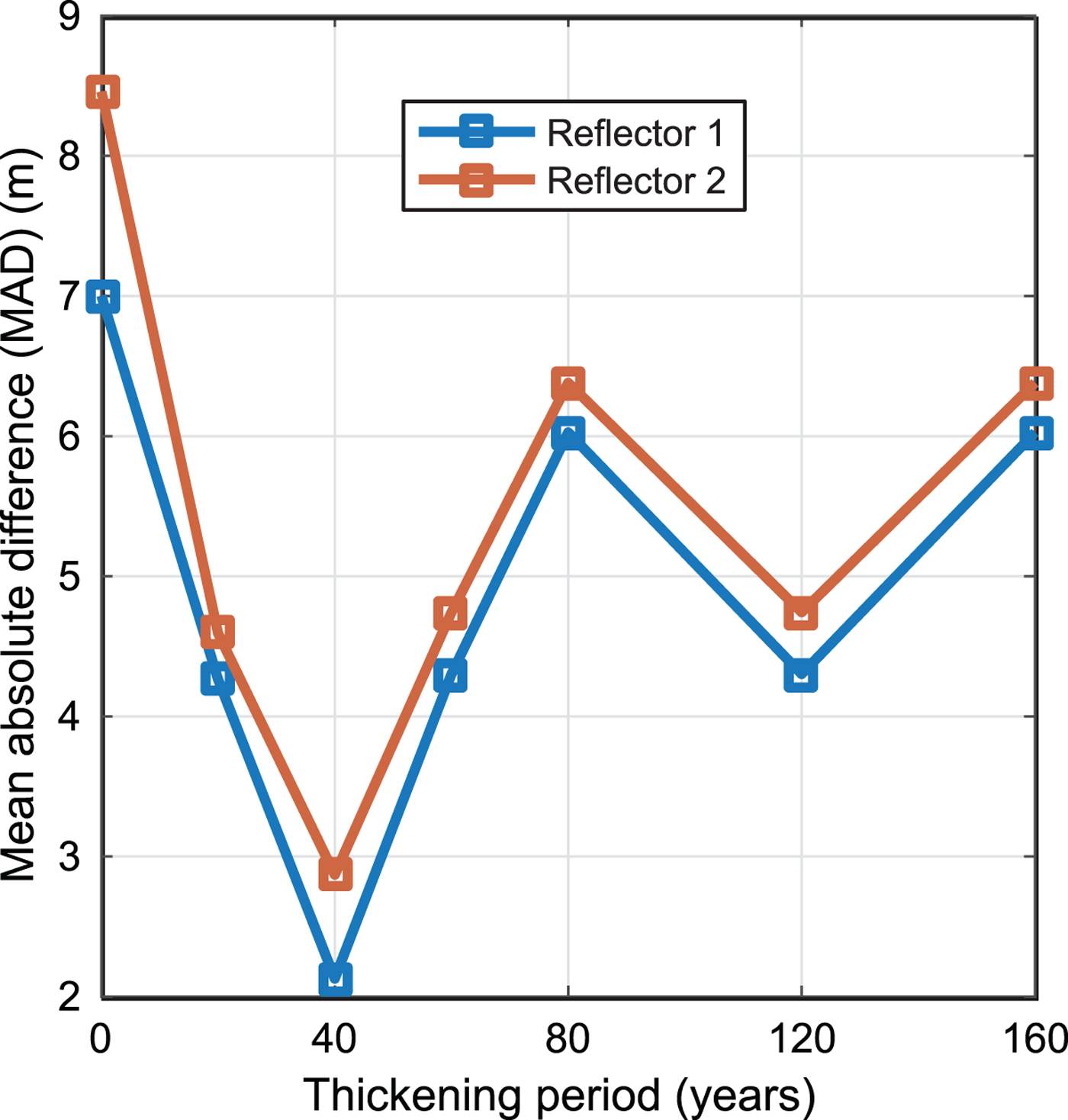
Fig. 5. Quality of fit for model measured as the mean absolute difference (MAD, Eqn (2)) for a range of thickening periods and n = 4.5. Reflector 1 is the shallowest with the mean measured depth of 27 m; reflector 2 has a mean depth of 48 m.
To quantify the quality of a match between the observed reflectors and the modelled isochrones, we measured the difference D in elevation as
 $$D = H_{\rm r}-H_{\rm i}.$$
Here, H r and H i are the (observed) reflector and (modelled) isochrone elevations, respectively. Their difference D is evaluated at N points along a reflector, where values of H r are available. A nominal distance between the adjacent points is 10 m. H r is affected by uncertainty in radio-wave propagation speed. However, because we selected an isochrone that best matches with the radar reflector, location-independent uncertainty in the propagation speed does not affect D. Relative uncertainty in D arises from lateral variations in the radio-wave propagation speed averaged between the surface and the reflector. Spatial variations in surface density are ~±2.5% on this ice rise (Goel and others, Reference Goel, Brown and Matsuoka2017), yielding an uncertainty in relative elevation (i.e., the shape of the reflector) of 0.1–0.3 m, depending on the reflector depths. We defined the mean absolute difference (MAD) for each radar reflector:
 $$MAD = \sum \displaystyle{{\vert D \vert } \over N} = \; \sum \displaystyle{{\vert {H_{\rm r}-H_{\rm i}} \vert } \over N}.$$
Because our model's isotropic-ice assumption does not apply well near the summit, we excluded the summit region (within 4 times the ice-thickness away from the ice flow divide). However, the exception is the shallowest two reflectors that have depths of 28 and 50 m near the summit. Over this depth range, the reflectors show upward arches with arch amplitudes that increase linearly with depth (Fig. 5 in Goel and others, Reference Goel, Brown and Matsuoka2017). It means that the primary process to generate these shallow arches is not anomalous vertical strain near the divide (Raymond effect) but rather an anomalously small SMB (Vaughan and others, Reference Vaughan, Corr, Doake and Waddington1999). We also excluded the region 2 km from both the downstream boundaries, as this region is subject to large errors from boundary conditions (Hvidberg, Reference Hvidberg1996). In the model, we use the thickening rates of 0.52 mieq a−1 for the northern flank and 0.57 mieq a−1 for the southern flank. Deeper reflectors are not examined because they are significantly older (>180 years, assuming SMB1) than the thickening periods considered here. The ages of the reflectors are estimated based on the ages of isochrones that match them best. Hence, these estimates are subject to input SMB used in the model. We find that the two shallowest reflectors (dated ~30 and ~60-year-old using SMB1) show very similar trends as the thickening period changes. Figure 5 shows that MAD decreases when the thickening period increases from zero to several decades. However, MAD then increases when the thickening period is extended longer, tripling for an 80-year-long thickening. For both reflectors, having thickening begin ~40 years before 2014 produced the best match (Fig 4). Differential thickening could cause the summit to migrate southwards, but we do not observe such a feature in the radargram. We conclude that it is very likely that the thickening started recently, sometime within the last century.
3.3 Past changes in SMB
The modelled isochrones match well with the two shallowest observed reflectors when the model is initialized with a steady-state ice rise with present-day SMB but slightly thinner, and then the ice rise is thickened for ~40 years. However, we find that the deeper reflectors are not replicated well (Fig. 4), and this discrepancy is more prominent in the northern flank.
To further examine this differential feature, we picked isochrones corresponding to eight radar reflectors (labelled 3–10 in Fig. 2) that gave the smallest MAD in the southern flank, 2–6 km away from the summit. Then we evaluated the matches between these selected isochrones and radar reflectors in the northern flank. We could have instead used the radar reflectors in the northern flank as references, but we found that approach to give worse matches than the case we present below.
For the case shown in Figure 4b, the values of D show that the reflectors in the southern flank are well replicated (|D| < 3 m), but the reflectors in the northern flank do not match well. This case is for an initial steady-state ice rise with the present-day SMB, but thinner than the present ice rise by ~20 m, that is then allowed to thicken for 40 years with a rate of 0.52 mieq a−1 on the northern flank and 0.57 mieq a−1 on the southern flank. This case which best fits the present-day ice flow speeds and two shallowest reflectors (Sections 3.1 and 3.2). However, the older isochrones consistently appear deeper than the reflectors, with MAD ranging between 10 and 20 m in the northern flank.
Here, we examine two hypotheses that might help explain the deeper isochrones in the northern flank. The first hypothesis is that past thinning occurred only on the northern flank. The other hypothesis is that SMB in the northern flank was smaller in the past than the present-day value while SMB in the southern flank remained unchanged. For both hypotheses, the modelled isochrones should appear at shallower depths and better match the reflectors. We can reject the first hypothesis because such a spatially restricted thinning would have caused the summit to migrate southward, which contradicts what the Raymond arches show (stable summit position or small migration northward).
The remaining hypothesis is that only the northern flank had smaller SMB in the past. To test this, we ran steady-state experiments for a thinner ice rise (prior to the recent thickening) assuming SMB values in the southern flank are equal to the observed present-day values, but smaller SMB values on the northern flank. All the other boundary conditions and model setups remain the same as the previous experiments. After reaching steady state (40T years), we changed the SMB in the northern flank to the present-day value. The outgoing flux is adjusted so that the ice rise is thickened for 40 years at a rate of 0.52 mieq a−1 in the northern flank and 0.57 mieq a−1 in the southern flank (Sections 3.1 and 3.2). The thickening rates and the period are not precisely determined with the previous experiments, but the shape of older reflectors #3–#8 are not sensitive to these factors. We ran four experiments with the shifted SMB values: ΔSMBnorth = SMBpast – SMBpresent = −0.05, − 0.1, − 0.15 and −0.2 mieq a−1 on the northern flank and adjusted the mass outfluxes to maintain a steady state.
Among these four values, we found the overall best fit with ΔSMBnorth = −0.1 mieq a−1. Figure 6 shows the resulting modelled isochrones for this case. Considering individual reflectors, the best matches occur for middle reflectors #4–#9 (see reflector labels, Fig. 2) with ΔSMBnorth = −0.1 mieq a−1, having MAD values 6–16 m smaller than those from other ΔSMBnorth values (Fig. 7). For SMB1 as input, reflectors #4–#9 are ~230–740 years old. For reflector #3 (age ~180 years), the two smaller ΔSMBnorth cases (−0.05, and − 0.1 mieq a−1), as well as the experiment presented in Section 3.2 (i.e. ΔSMBnorth = 0), produce similarly small values of MAD, but the larger two ΔSMBnorth cases give much larger MAD values. For the deepest reflector #10 (age ~1100 years), MAD decreases strongly when ΔSMBnorth changes from 0 to −0.15 mieq a−1, and then MAD increases when the ΔSMBnorth value decreases further.
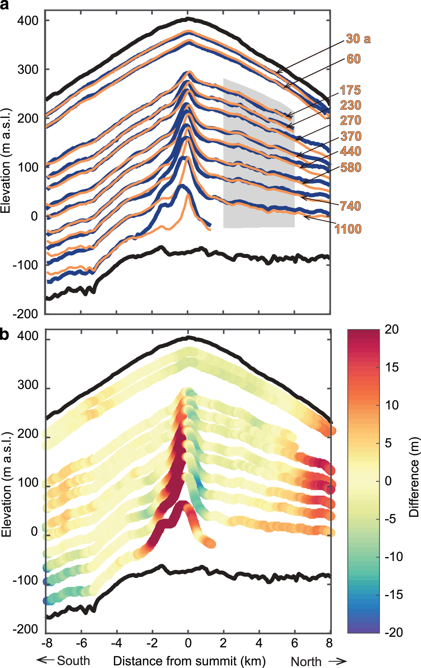
Fig. 6. Modelled stratigraphy for experiment with smaller SMB values in the northern flank. For this experiment, SMB in the southern flank was unchanged, but the SMB in the northern flank was reduced by 0.1 mieq a−1 (ΔSMBnorth = −0.1 mieq a−1). (a) Observed reflectors and modelled isochrones as in Figure 4. Grey region on the northern flank was used to calculate MAD in Figure 7. Orange labels show ages of the modelled isochrones in years (estimated using a model with SMB1). (b) Elevation difference D as in Figure 4.
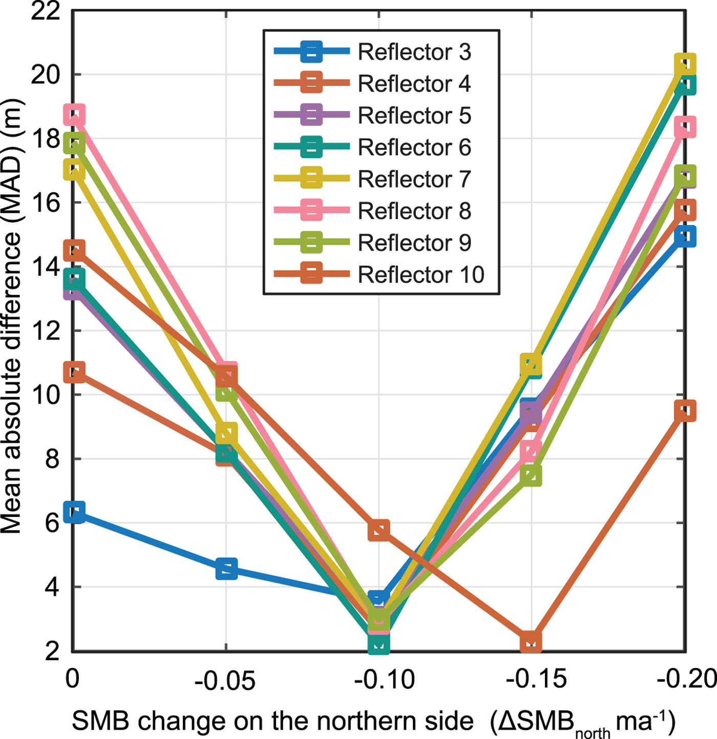
Fig. 7. Quality of fit for model MAD (Eqn (2)) in terms of past SMB changes over 1200 years in the northern flank, ΔSMBnorth. Reflector 3 is shallowest/youngest, whereas reflector 10 is deepest/oldest.
Based on these experiments, we propose the following history of SMB in the northern flank. (i) Prior to 1100 years BP, it was smaller than the present value by 0.15 mieq a−1. (ii) Between 740 and 1100 years BP, it increased to 0.1 mieq a−1 smaller than the present value. (iii) Between 230 and 740 years BP, it remained unchanged. (iv) Since 230 years BP, it increased gradually (by 0.1 mieq a−1) to the present value, reaching the current SMB value ~40 years ago.
This proposed history is, however, not unique as the ages of the radar reflectors are not constrained by the field observations. In particular, the observed reflector patterns can be replicated as long as one keeps the same north–south contrast in the past SMB. For example, we can obtain results similar to the one presented in Figure 6 (i.e., ΔSMBsouth = 0, ΔSMBnorth = −0.1 mieq a−1) by using a combination of ΔSMBsouth = +0.05 mieq a−1 and ΔSMBnorth = −0.05 mieq a−1 or another combination of ΔSMBsouth = +0.1 mieq a−1 and ΔSMBnorth = 0. Nevertheless, with all these possible histories, the SMB contrast between the north and south flanks was stronger by 0.1 mieq a−1 in the past ~230–740 years.
4 DISCUSSION
4.1 Model uncertainty
Results presented so far involved the use of Glen's rheological power index n = 4.5, a value used by Gillet-Chaulet and others (Reference Gillet-Chaulet, Hindmarsh, Corr, King and Jenkins2011) to describe ice rheology at the Greenland summit. The other widely used value is n = 3 (e.g., Cuffey and Paterson, Reference Cuffey and Paterson2010). The n = 3 value likely gives a better approximation of the ice rheology in the flanks of our domain, whereas n = 4.5 is the best isotropic approximation near the flow divide. Our study area lies between the flanks and divide, being 4–12 times the ice-thickness (2–6 km) away from the flow divide. To examine the sensitivity of our results to this uncertainty in ice rheology (Kingslake and others, Reference Kingslake2014), we also ran the model for n = 3 and found that the main results stay the same though some details change. We discuss these details next.
Experiments using n = 3 give the best agreement with observed flow speeds when the current thickening rate is 0.54 mieq a−1 on the northern and 0.61 mieq a−1 on the southern flank (Fig. 3). These values are 5–10% larger than those for n = 4.5. For the periods of recent thickening, MAD decreases as the thickening period approach 20 years, but then increases as the period increases further (Fig. 8). The MAD minima occur at 20 years, which is shorter than the 40 years for n = 4.5 (Fig. 5). Therefore, although the exact rate and period of current thickening depend on the ice model, both models agree that the current thickening started only in the past few decades, not for the entire past century.
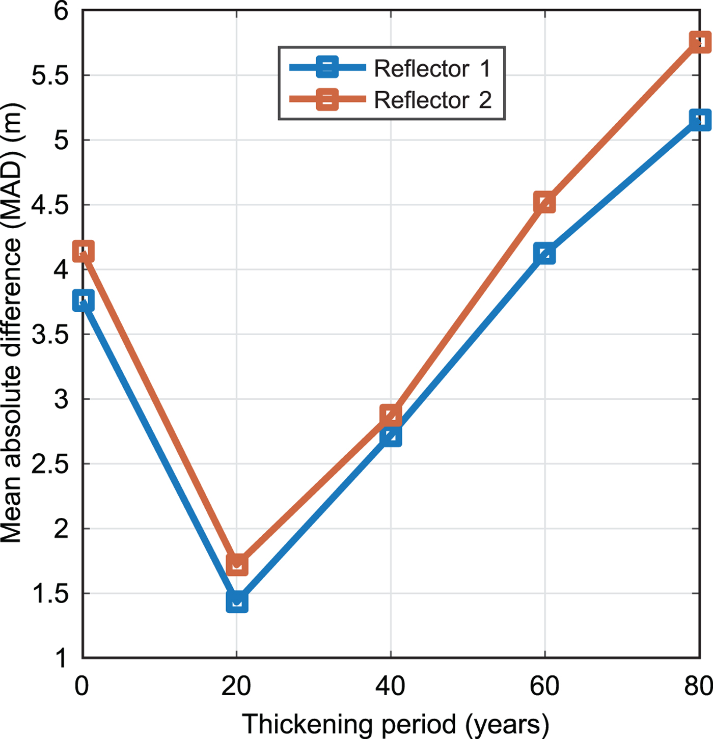
Fig. 8. Quality of fit for model MAD over a range of thickening periods, the same as Figure 5 except for Glen's rheological power index n = 3.
Similarly, our main conclusions on the past SMB changes are the same as those for n = 4.5 (Fig. 9). In particular, for n = 3, MAD is minimized when ΔSMBsouth is ~ − 0.1 mieq a−1. Also, the shallower reflector #3 gives a smaller MAD when ΔSMBsouth is larger (−0.05 mieq a−1), whereas the deeper reflector #10 gives a smaller MAD when ΔSMBsouth is smaller ( − 0.15 mieq a−1). Therefore, past SMB changes and their timing remain essentially unaffected by rheology uncertainties. We observe that MAD values are slightly lower in the n = 3 experiment for the middle reflectors (#4–#9) when ΔSMBsouth is − 0.05 and − 0.15 mieq a−1. This feature may indicate a more gradual transition in SMB.
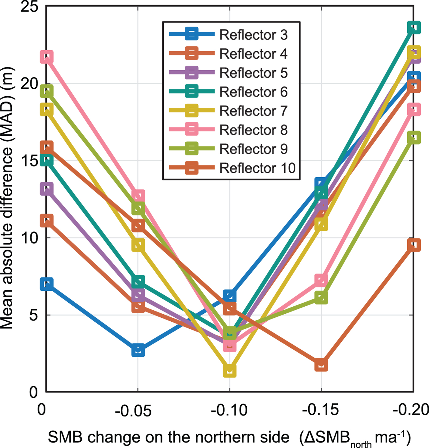
Fig. 9. Quality of fit for model MAD in terms of past SMB changes, the same as Figure 7 except Glen's rheological power index n = 3.
Overall, on comparing isochrones of the same ages for the two rheological cases, the differences were limited to the divide region (within 2–3 times the ice-thickness from the summit), with n = 4.5 producing larger Raymond arches. Our experiment on the onset of thickening evaluates MAD for the shallow reflectors in the divide region, and thus it is affected by the changes in rheology, whereas other results do not.
These results show that our main findings in Section 3 depend only slightly on the choice of the ice rheology. However, the more recent changes recorded in the shallower part of the ice do change with n despite shallow ice being less affected by ice deformation. A possible explanation is the sensitivity of the surface slope to rheology. A larger n has a more nonlinear relationship between strain and stress, yielding larger Raymond arches, stiffer ice near the divide, and steeper surface slopes in the flank. This n-dependent feature in the surface topography could result in similar features in the elevations of shallow reflectors. In this way, more recent ice can be more sensitive to the choice of n.
Figures 4 and 6 show that deep reflectors (except for the shallowest two) do not match well in the divide region. The minimum MAD reaches 12 m in Figure 4 and 16 m in Figure 6 in the divide region, which is a magnitude larger than the MAD values for the best cases in the flank. This affirms our decision of excluding this region from evaluation.
Finally, we consider that the model neglects the flow divergence that must occur over the ice rise. Flow divergence can reduce or eliminate the Raymond effect under the flow-divide (Martín and others, Reference Martín, Hindmarsh and Navarro2009b). We excluded this region from most of our analysis, so this should have little effect on our results. Passalacqua and others (Reference Passalacqua2016) demonstrated that for a diverging flow the age of the ice can be overestimated, resulting in shallower isochrones. This effect is stronger in the region close to the surface, and thus may affect our result on the onset of thickening slightly. However, the small asymmetry in divergence along the modelled profile (Section 2.2), should not affect our main finding regarding the changes in SMB asymmetry over the past millennia.
4.2 Present-day SMB uncertainty
The SMB prescribed in the above experiments (SMB1 in Fig. 2a) assumes that the density varies only in the vertical, not in the lateral. Goel and others (Reference Goel, Brown and Matsuoka2017) also presented a second estimate of SMB, labelled SMB2 in Figure 2a, which accounts for both vertical and lateral variability in density but neglects temporal variations in SMB over the last decade. SMB1 and SMB2 values are estimated using different assumptions, with neither set of assumptions clearly better than the other. Therefore, we repeated all of the above experiments with the SMB2 estimate as input. We found that with the SMB2 dataset, the observed flow speeds were best replicated when the ice rise thickened at a rate of 0.4 mieq a−1on both slopes. This thickening rate is smaller than the results presented above (0.52–0.57 mieq a−1, Section 3.1), but closer to our previous estimate using the input-output method and SMB1 for the last decade (0.16–0.30 mieq a−1; flowline setup; Goel and others, Reference Goel, Brown and Matsuoka2017). Nevertheless, estimates of thickening periods and past SMB changes remain virtually the same, regardless of the SMB inputs. However, because SMB2 is smaller than SMB1, the ice is correspondingly older by 6–10% and thus the inferred SMB changes in the past happened earlier.
For the range of n and the input SMB, our modelling results show that Blåskimen Island is at present thickening at a rate of 0.4–0.6 mieq a−1. This model estimate is about twice the mass-balance estimate obtained along this profile using the input–output method from the field data (0.16–0.30 mieq a−1; flowline setup; Goel and others, Reference Goel, Brown and Matsuoka2017). Those estimates with the input–output method range from 0 to 0.6 mieq a−1 among the six columns along this profile. Different sets of assumptions used in these methods probably lead to this range of estimated thickening rates. Nevertheless, both estimates indicate that the ice rise is thickening, neither steady state nor thinning.
As we do not have any independent information on past SMB changes in this region, we do not know if the changes in SMB were sudden or gradual. But depending upon the actual scenario, steady-state and transient simulations can lead to slightly different results. For this study, we use steady-state simulations and present sensitivity tests to show the uncertainty in our final results.
4.3 Possible causes of recent thickening
Possible causes of the recent thickening of the ice rise include a decrease in outgoing mass flux, an increase in SMB, or a combination of these two. We examine these causes next.
The outgoing ice flux around the ice rise is regulated by the slope of the grounding line and the amount of buttressing given by the adjacent ice shelf. Presently, no ice shelf abuts the northern flank (Fig. 1), so the only possible change on the northern flank would be a reduction of buttressing in the past. As such a reduction would lead to thinning, not thickening, we conclude that changes to the northern flank cannot explain the recent thickening. Considering the other three sides, the ice rise faces different ice shelves with distinct characteristics. On the west, the Jelbart Ice Shelf is fed by the Shytt Glacier and moves relatively fast (~400 m a−1; Rignot and others, Reference Rignot, Mouginot and Scheuchl2011), whereas on the east and south, the ice shelves move very slowly (<50 m a−1; Rignot and others, Reference Rignot, Mouginot and Scheuchl2011). But we previously found that the ice thickening is fairly uniform over the entire ice rise (Goel and others, Reference Goel, Brown and Matsuoka2017). Given the nonuniformity of buttressing, we argue that any decrease in mass outflux is unlikely to be the main driver of the recent thickening of the ice rise.
The other possible cause is an increase in SMB. To examine this cause, we consider ice cores near the ice rise. In the immediate vicinity, the 23 m-long firn core obtained from Blåskimen Island, dating back 17 years from 2014, shows an overall increase in SMB, but the trend was not statistically significant due to large interannual variabilities (Vega and others, Reference Vega2016). Two more ice cores were drilled in the adjacent ice rises to the east, Kupol Moskovskij and Kupol Ciolkovskogo (Fig. 1). Kupol Moskovskij shows a trend similar to Blåskimen Island, whereas Kupol Ciolkovskogo shows a long-term decrease in SMB. Further east, an ice core from Derwael Ice Rise in eastern DML, ~1000 km east of Blåskimen Island, shows that SMB increased there by 32% over the past five decades (Philippe and others, Reference Philippe2016). There are five more ice cores from the coastal DML (three drilled on the ice shelves and two on the ice sheet); all of which show a decreasing SMB over recent decades (Thomas and others, Reference Thomas2017). Overall, these SMB records in coastal DML indicate high variability among adjacent ice rises, ice shelves and coastal parts of the ice sheet.
Regional-scale climate modelling in this region show that SMB variations arise from variations in precipitation and wind erosion, with smaller contributions from sublimation and snowdrift (Lenaerts and others, Reference Lenaerts2014). The strong topographic gradients over an ice rise lead to the observed upwind–downwind contrast in SMB. From our analysis, Blåskimen Island has thickened over the past ~40 years, and differences in thickening may affect the contrast. However, the thickening-rate difference between northern and southern flanks in SMB is only 10%, which results in only a 2 m difference in elevation over 40 years. Therefore, the ice rise has maintained a similar topography to today but was thinner by ~20 m. Thus, any change in the orographic effect associated with a topography change is probably too small to significantly alter the SMB patterns.
4.4 Ice dynamics and SMB changes
We have shown that, during the period before ~40 years ago, the upwind−downwind (north−south) SMB contrast across the ice rise was higher. Our simulations suggest that the ice rise was in steady state over this period, so the changes in SMB are not associated with changes in ice-rise topography, but more to regional atmospheric changes.
Our data show that north–south contrast in SMB was larger in the past. However, our modelling approach cannot readily distinguish between the following cases: (1) the past SMB was higher than the present-day SMB on the southern flank. (2) The past SMB was lower than the present-day SMB on the northern flank. And (3), a combination of both cases. The ice rise was maintained in a steady state in this period, allowing Raymond arches to form. Thus, the ice fluxes must have adjusted in accordance to the SMB. Considering the boundaries, the northern downstream boundary is free of any ice shelf, thus outflux to the north could have responded to maintain a steady state. In contrast, the southern downstream boundary faces an ice shelf and it is unlikely to have coincidentally changed just the right amount to maintain a steady state with the changing SMB. Therefore, we argue that the majority of SMB changes happened in the northern flank; that is, case (2) is likely the major cause of the observed SMB contrast. But for this argument to hold, we have to assume that the northern flank did not have an ice shelf in the past. Thus, we suggest that the northern side of this ice rise has been free of an ice shelf in the recent past.
The SMB contrast on Blåskimen Island is oriented northwest–southeast (Fig. 5 in Goel and others, Reference Goel, Brown and Matsuoka2017). This direction is along that of the prevailing wind instead of the north-easterly moisture source (Lenaerts and others, Reference Lenaerts2014), which indicates that wind-driven processes affect the SMB of this ice rise. Consistent with this argument, during the field campaign we found that the northern flank had much larger sastrugi, the southern flank being much softer and smoother. Therefore, we speculate that lower SMB in the northern flank was caused by stronger winds. Overall, a stronger wind may cause more orographic precipitation on the southern flank (Frezzotti and others, Reference Frezzotti2004), which would contribute to the larger north–south SMB contrast in the past.
Our work suggests that ice-rise evolution may be affected more strongly by wind and SMB than by adjacent ice shelves. Such a strong dependence on SMB has three major consequences. First, SMB changes faster than changes in ice shelves (except for iceberg calving). On ice rises, small changes can be amplified by the orographic effect. So, SMB-driven changes in ice rises can happen faster than most ice-dynamics-driven changes. Second, SMB changes are closely related to atmospheric circulations, which can be highly variable. The coastal DML receives ~50% of all of its yearly precipitation through about eight storm events (Reijmer and van den Broeke, Reference Reijmer and van den Broeke2003; Schlosser and others, Reference Schlosser2010). Thus, SMB in the coastal region is affected by the trajectories, frequencies and transported moisture from major storms, which are subject to influences from synoptic atmospheric circulation. Local sources of moisture are often coastal polynyas, found on the western (downwind) side of a nearby ice tongue. Polynya distribution depends on ocean temperature as well as the extent of ice tongues, which can be highly variable. Finally, if SMB changes are driven by the atmosphere, they can happen over a large area (e.g., DML) and thus many ice rises there can be affected similarly. Under similar SMB forcings, however, the evolution of individual ice rises can be quite different because their glaciological settings can be highly variable. Hence, it is important to examine more ice rises in this region to clarify how SMB and ice-shelf dynamics contribute to the ice-rise evolution and in turn change buttressing to the ice sheet.
5 CONCLUSIONS
Using a thermo-mechanically coupled Elmer/Ice flow model, we examined the evolution of Blåskimen Island, western DML, in East Antarctica. We found that this ice rise is presently thickening at a rate of 0.4–0.6 mieq a−1. The thickening began ~20 − 40 years ago, before which the ice rise was in a steady state but had a different SMB distribution than at present. Presently, the ice rise receives more SMB in the southern, upwind flank than on the northern flank. We found that this upwind–downwind contrast was stronger in the past by 23% (or 0.15 mieq a−1) before ~1100 years. Since then, this contrast has been decreasing, apart from a period of constant contrast between ~230 and ~740 years ago. The driver of these persistent changes in SMB remains uncertain, but the evidence indicates it is more likely due to changes in wind and the moisture source, rather than local ice-rise topography. Our work indicates that SMB in the past can leave distinct spatial patterns in ice stratigraphy, which can be investigated by a combination of radar profiling, shallow ice cores and ice flow modelling. Along the DML coast, there are numerous ice rises near the calving front and their evolution is largely unknown. These ice rises should be studied to determine the spatial pattern of SMB and whether their past changes are driven mostly by SMB or by ice-shelf dynamics. Our technique effectively assimilates geophysical data in an ice rise, avoiding the complexity of ice flow and rheology at the divide and thus may be used to better understand these ice rises.
AUTHOR CONTRIBUTIONS
All three contributed to design this study and interpret the model results. Goel conducted the experiments together with Martin. Goel and Matsuoka prepared the manuscript and Martin contributed to finalize it.
ACKNOWLEDGEMENTS
This work was funded by grants from Norwegian Antarctic Research Expeditions (NARE) and the Center for Ice Climate and Ecosystems (ICE) of the Norwegian Polar Institute. Vikram Goel received a PhD studentship from National Centre for Antarctic and Ocean Research (NCAOR), through a financial support (MoES/16/22/12-RDEAS) from the Ministry of Earth Sciences (MoES), Government of India. The model is based on the open-source code Elmer mainly developed by the CSC-IT Center for Science Ltd in Finland. We thank Joel Brown and Reinhard Drews for their help with setting up the model. We thank the two anonymous reviewers and the editor Michelle Koutnik for their constructive comments, which improved the manuscript significantly. Figure 1 was developed using a free GIS data package Quantarctica (quantarctica.npolar.no). This is NCAOR contribution No. 49/2018.


 Open access