


1. Introduction
Cow–calf production is the foundation of the United States beef industry. Second only to land, the cow herd represents a major capital investment for beef production.Footnote 1 In 2019, there were nearly 32 million head of beef cows spread across roughly 730 thousand operations (USDA-NASS, 2017; 2020). A simple average price for bred replacement cows and heifers in 2019 from a sample of locations across the United States is approximately $911/head (LMIC, 2020; MDAC, 2020).Footnote 2 This translates into roughly $29 billion intermediate-term asset value (asset life ≤ 10 years). Specific to the roughly 477,000 head in Mississippi averaging $857/head this translates to $403 million in intermediate-term asset value (MDAC, 2020).
Breeding females (BF) within and across herds in the United States are extremely heterogeneous in genetic makeup. This result is primarily driven by the additional productivity and longevity reported for crossbred females over their purebred counterparts (Weaber, Reference Weaber2010), and more importantly, the wide variation in climatic environments and resource availability in which cow herds must adapt and prosper. The vast degree of heterogeneity of the United States cow herd makes buyer asset valuation difficult.
Numerous economic studies have reported feeder cattle hedonic valuation to backward inform cow–calf producers of the market demand for various physical and genetic characteristics of their output. However, scant economic research has been published regarding the demand for the characteristics of BF (cows and heifers), the primary source of herd valuation. Their total asset value is not entirely derived from the characteristics passed on to their calves as reproductive success is also a factor. Three closely related beef cow characteristics demand studies have been published in economic literature since 1990: mixed slaughter and BF in Kansas (Mintert et al., Reference Mintert, Blair, Schroeder and Brazle1990), cow–calf pairs in Kansas (Parcell, Schroeder, and Hiner, Reference Parcell, Schroeder and Hiner1995), and pregnant BF in Oklahoma (Mitchell, Peel, and Brorsen, Reference Mitchell, Peel and Brorsen2018).Footnote 3 The first two are based primarily on group averages (as is typical of western auction sales) and the last on aggregated Agricultural Marketing Service data. Due to the data limitations, the previous research was unable to control for individual-specific attributes, primarily those related to reproductive success. A breeding female’s reproductive success is defined as her ability to conceive, carry a live calf to term, birth, and wean a live calf. Not fully accounting for reproductive success when investing in BF can have long-run effects on the profitability and productive success of a producer’s cow–calf operation (Parcell et al., Reference Parcell, Randle, Kerley, Patterson, Smith and Olson2003).
When purchasing pregnant females, abortion risk is a major concern. Abortion is defined as the early termination of pregnancy, and a breeding female is at risk from conception until she is 260 days pregnant (Thurmond, Picanso, and Jameson, Reference Thurmond, Picanso and Jameson1990). A pregnant female has the highest probability of aborting her calf through early and mid-gestation, with a slight increased risk immediately prior to birth (Forar et al., Reference Forar, Gay, Hancock and Gay1996; Silke et al., Reference Silke, Diskin, Kenny, Boland, Dillon, Mee and Sreenan2002; Santos et al., Reference Santos, Thatcher, Chebel, Cerri and Galvão2004; Lonergan et al., Reference Lonergan, Fair, Forde and Rizos2016). Because abortion presents a significant financial loss to the producer (Peter, Reference Peter2000; Hovingh, Reference Hovingh2009), buyers of BF are expected to account for the probability she will carry the calf to term. A higher expected risk of abortion (i.e. earlier in gestation) at the time of sale is likely to reduce bids, hence, reducing the revenue for the seller.
The goal of this research is to provide a more detailed assessment of cow herd asset valuation. To achieve this goal, the research conceptually and empirically identifies the impacts of a richer set of individual physical characteristics known to impact reproductive success. These factors include, but are not limited to (i) simultaneously controlling for pregnancy and months pregnant to identify the associated risks of abortion, (ii) proven success with a calf on her side, (iii) birthing due dates and the associated risks of dystocia and new born death loss, (iv) udder and teat condition impacting milk production and ease of calf nursing, and (v) locomotion and its impacts on expected asset longevity.
The remainder of this research is laid out as follows. First, a conceptual characteristics-based asset value model for BF is developed from which a priori expectations regarding reproductive success characteristics are derived. Second, the data and a priori expectations are developed from economic and production literatures. Third, the hedonic cross-sectional time series attributes of the data are discussed, and the empirical strategy identified. Fourth, the marginal implicit values of characteristics are provided. Finally, conclusions and implications are discussed.
2. Conceptual Asset Value Model
BF are a capital investment for the cow–calf operation as an input into the production of beef. Because reproductive success and productivity of BFs are not observable at the time of purchase, buyers must form beliefs as to the female’s net present value (NPV) given the signals provided by her observable characteristics. The buyer’s total value belief is a function of the sum of the discounted net expected cash flows of all possible calves produced and the BF’s expected future salvage value. The total value belief is derived, in part, from the sum of the expected marginal value yields of observed characteristics at the time of bidding. As any given characteristic’s net marginal value product signal increases, so too does the buyer’s total value signal and subsequent bid under any informational assumption in English auctions.
Before developing a more detailed conceptual characteristics-based asset valuation model, an age-based (life cycle) asset valuation model is first presented. The general expected NPV for  $n \in N$ heterogeneous risk neutral buyers of the $i \in I$ BF at auction is identified as
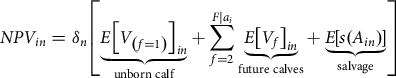 $$NP{V_{in}} = {\delta _n}\left[ {\underbrace {E{{\left[ {{V_{\left( {f = 1} \right)}}} \right]}_{in}}}_{{\rm{unborn\ calf}}} + \sum\limits_{f = 2}^{F|{a_i}} {\underbrace {E{{\left[ {{V_f}} \right]}_{in}}}_{{\rm{future\ calves}}} + \underbrace {E\left[ {s({A_{in}})} \right]}_{{\rm{salvage}}}} } \right]$$
where  ${\delta _n}$ is the buyer’s discount factor. For clarity, time subscript notations are suppressed for purchase date, as well as expected future births and sales across calves which are assumed unique to each buyer’s planning horizon. If pregnant at the time of sale, the expression $E{\left[ {{V_{\left( {f = 1} \right)}}} \right]_{in}}$ is the buyer’s expected net value of the unborn calf. If not pregnant, this expression equals zero. The unborn calf is indexed as $f = 1$, as the first out of $F|{a_i} = {A_{in}} - {a_i}$ expected future calves remaining in the BF’s expected productive lifespan ${A_{in}}$, given her current age ${a_i} \in [1,2,,,{A_{in}}]$. All expected future calves are indexed $f \in [2,3,,,F|{a_i}]$. The sum of the expected net values of future calves $\sum\limits_{f = 2}^{F|{a_i}} {E{{\left[ {{V_f}} \right]}_{in}}} $ and the expected salvage value $E\left[ {s({A_{in}})} \right]$ comprises the remainder of the BF’s total expected asset value for each buyer.
Equation (1) can be further detailed by including the impacts of a BF’s observed set of physical characteristics  ${K_i}$ to the buyer at time of sale which provide signals for buyer valuation. Given some of the dam’s characteristics are expressed in her calves to some degree (Parish, Reference Parish, Williams, Coatney, Best and Stewart2018), some subset of dam characteristics ${k_i} \subseteq {K_i}$ represents signals of her unborn and future calves’ characteristics $\kappa ({k_i})$, where $\kappa '({k_i}) \gt 0$, contingent on known or expected sire characteristics. For example, heavier muscling observed in a BF is expected to increase the expected muscling expressed by her calf. The remaining set of characteristics pertaining only to the female’s reproductive success and not the calf’s expected value is ${r_i} = {K_i} - {k_i}$; examples include laminitis and the BF’s udder condition at the time of sale.
A characteristics-based expected net value of the unborn calf in equation (1) is
 $$E{\left[ {{V_{\left( {f = 1} \right)}}} \right]_{in}} = P{\left( {{{\bf{K}}_i}} \right)_n}E{\left[ {R\left( {{\bf{v}},{\bf{\kappa (}}{{\bf{k}}_i}{\bf{)}}} \right) - C\left( {{{\bf{K}}_i}} \right)} \right]_{n,\left( {f = 1} \right)}} - \left( {1 - P{{\left( {{{\bf{K}}_i}} \right)}_n}} \right)E\left[ {OC\left( {{{\bf{K}}_i}} \right)} \right]{}_{n,\left( {f = 1} \right)}$$
The expression  $P{\left( {{{\bf{K}}_i}} \right)_n}$ is the individual buyer’s joint subjective probability of selling the unborn calf if the BF is pregnant, after surviving successive stages of production each containing unique risk factors, such as abortion, dystocia (calving difficulty), and disease/injury after birth.Footnote 4 The joint probability is a function of a vector of reproductive success characteristics possessed by the BF. Examples of reproductive success characteristics are months pregnant (Lonergan et al., Reference Lonergan, Fair, Forde and Rizos2016), body condition (Parish and Rhinehart, Reference Parish and Rhinehart2008), and age (Herring, Reference Herring1996). The expression $E\left[ {R\left( {{\bf{v}},{\bf{\kappa (}}{{\bf{k}}_i})} \right)} \right]$ is the buyer’s expected return from the sale of the unborn calf. Expected return is a function of the vector of expected trait levels passed from dam to calf ${\bf{\kappa (}}{{\bf{k}}_i})$, as well as their corresponding expected implicit marginal values ${\bf{v}}$ paid by feeder cattle buyers. Examples are breed composition, frame, and muscle score and have been extensively analyzed in the feeder cattle input characteristics demand literature (e.g., Schroeder et al., Reference Schroeder, Mintert, Brazle and Grunewald1988; Turner, Dykes, and McKissick, Reference Turner, Dykes and McKissick1991; Coatney, Menkhaus, and Schmitz, Reference Coatney, Menkhaus and Schmitz1996; Barham and Troxel, Reference Barham and Troxel2007; Zimmerman et al., Reference Zimmerman, Schroeder, Dhuyvetter, Olson, Stokka, Seeger and Grotelueschen2012). The expression $E\left[ {C\left( {{{\bf{K}}_i}} \right)} \right]$ represents the buyers expected accrued production costs during gestation, birth, and production of the feeder calf. For example, increased overall body size (body weight × frame) of both cows and calves has been shown to increase daily production cost (Bir et al., Reference Bir, DeVuyst, Rolf and Lalman2018). The expression $\left( {1 - P{{\left( {{{\bf{K}}_i}} \right)}_n}} \right)$ is the buyer’s subjective probability of investment loss if the fetus/calf aborts/dies prior to marketing. The subsequent expression $E\left[ {OC\left( {{{\bf{K}}_i}} \right)} \right]$ represents the expected accrued production costs up to death or expected lost sales revenue. Therefore, $P{\left( {{{\bf{K}}_i}} \right)_n}$ must be sufficienty large relative to expected opportunity costs for postitive expected net returns to occur. This highlights the importance of the vector of reproductive success characteristics in buyer valuation of a pregnant BF.
Next, the expected net values of future calves are similarly calculated as the unborn calf. One notable addition to the buyer’s subjective probability reflects the expectation that the BF will conceive in the future, which is also a function of the female’s characteristic signals such as current pregnancy status, age, and body condition. The general form representation of equation (1) as a characteristics-based function is now
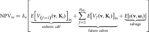 $${\rm NPV}_{{in}} = {\delta _n}\left[ {\underbrace {E{{\left[ {{V_{\left( {f = 1} \right)}}({\bf{v}},{{\bf{K}}_i})} \right]}_{in}}}_{{\rm{unborn\ calf}}} + \underbrace {\sum\limits_{f = 2}^{F|{a_i}} {E{{\left[ {{V_f}({\bf{v}},{{\bf{K}}_i})} \right]}_{in}}} }_{{\rm{future\ calves}}} + \underbrace {E\left[ {s({\bf{\nu }},{{\bf{\omega }}_i})} \right]}_{{\rm{salvage}}}} \right]$$
where the subset of observable characteristics to the buyer impacting salvage value is  ${{\bf{\omega }}_i} \subseteq {{\bf{K}}_i}$, as well as their corresponding expected implicit marginal values ${\bf{\nu }}$ paid by slaughter cow buyers. Examples of important salvage value characteristics are health, weight, and breed type that impact expected dressing percentage and subsequent red meat yield (Mintert et al., Reference Mintert, Blair, Schroeder and Brazle1990; Coatney, Shaffer, and Menkhaus, Reference Coatney, Shaffer and Menkhaus2012). In all, the buyers’ perceived total marginal value product of any characteristic’s contribution to the NPV is a complicated relationship of various characteristic combinations, some of which may simultaneously impact the buyers’ expected returns, production costs, and salvage value.
Finally, the cattle auctions analyzed herein utilize an English auction format, where supply is fixed in the short run. In such a setting, the buyer forms a value signal from the observable animal characteristics, private cost information, as well as input and output price forecasts. Regardless of the assumption of whether the buyer’s value information is common, private, affiliated, or interdependent, unilaterally higher valuations result in higher optimal bids (Krishna, Reference Krishna2002). If a particular characteristic is valued/devalued in a sufficiently similar manner by bidders, the observed price (second highest value  $NP{V_{i(2)}}$) is expected to increase/decrease, ceteris paribus, hence identifying the characteristic’s implicit localized market demand.
3. Data and A Priori Expectations
Because reproductive success and future calf values are not directly observable at the time of purchase, buyers must form beliefs based on signals provided from a visual assessment of the animal’s current physical characteristics (e.g., breed type, muscling, body and udder condition), current information provided by a veterinarian (e.g., health and pregnancy), and historical information provided by the seller (e.g., health and pedigree). In a typical commercial grade auction setting as analyzed herein, historical production and health information are rarely provided. Therefore, the observable characteristics and information provided by the auction’s veterinarian are the primary pieces of information regarding potential reproductive success for buyers to use to develop a partial signal toward her NPV.
Animal-related data collected for this research were strictly observed in a public setting. Therefore, approval from the Institutional Animal Care and Use Committee was not necessary. The data for this research were collected by trained livestock evaluators from May 5, 2014, to May 4, 2015, at seven stockyards scattered through northeast, southeast, and southwest Mississippi. As a condition for data collection, anonymity of stockyard locations is maintained. To collect the physical characteristics data within the short window of time it takes to sell an animal (roughly 30 s), trained evaluators worked in teams of two to three per sale (Parish et al., Reference Parish, Williams, Coatney, Best and Stewart2018). All evaluators were given a standardized key with defined characteristic levels to use throughout the collection process to minimize scoring discrepancies among evaluators.
Price and characteristics were collected for females whether destined for slaughter or breeding, as well as feeder calves. The auctioneer sold slaughter females on a $/cwt basis and BF on a $/head basis. After excluding observations with missing values, the BF data set analyzed consists of 3,571 individual observations. The average BF price per head was $1,569.06. Summary statistics and definitions of variables collected in this analysis are reported in Table 1. Novel variables of interest included in this analysis are expected calving date, subjective udder suspension and teat scores, temperament, locomotion, and concurrent auction slaughter cow and feeder calf prices. The following subsection details the data and develops a priori expectations in relation to the conceptual model expressed in equation (3) by relying on both production and economic literature. A summary of a priori expectations is provided in the results Table 2 for ease of comparison to empirical results.
Table 1. Variable definitions, scales, and summary statistics;  ${N_{obs}} = 3,571$ breeding females

a  ${N_{obs}} = 2,724$ for age; excludes broke, short, and no mouth cattle.
Table 2. Parameter estimates of breeding female hedonic model
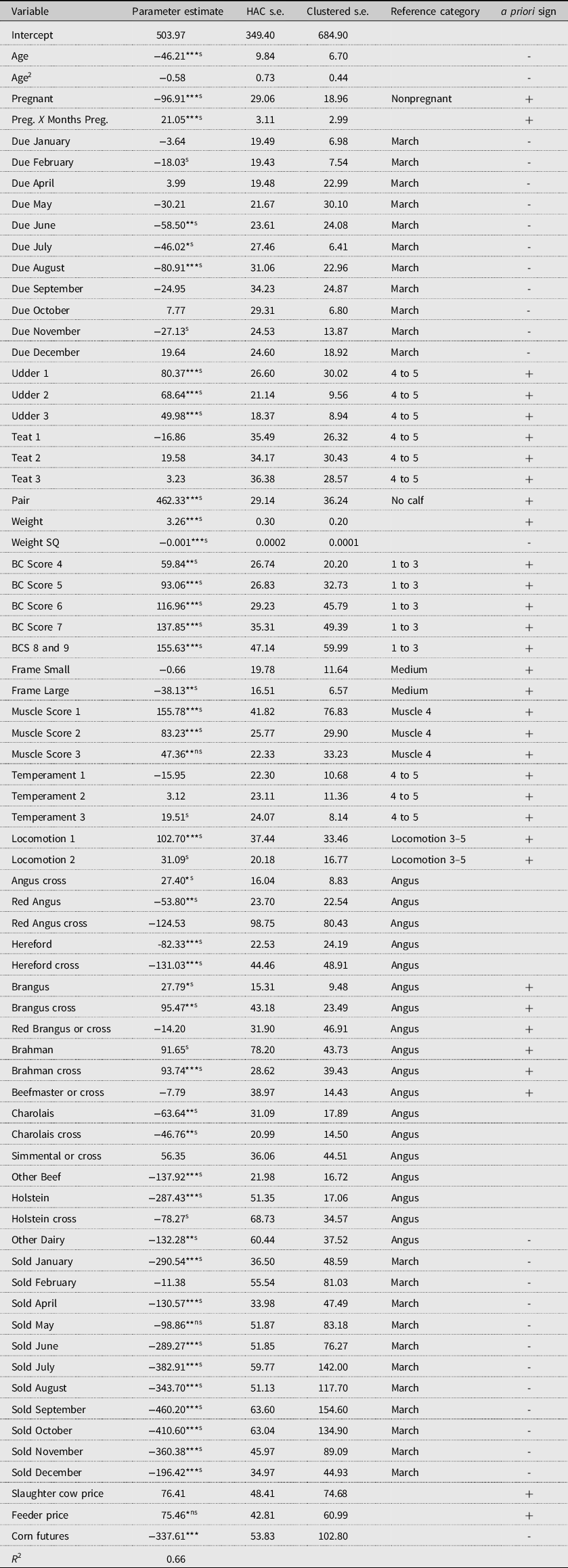
*** Significantly different from zero at significance level α = 0.01, ** at α = 0.05, and * at α = 0.10 using HAC standard errors.
s Significantly different from zero by at least significant level α = 0.10 using Clustered standard errors.
ns Not significantly different from zero by at least significant level α = 0.10 using Clustered standard errors.
3.1. Age
The first characteristic introduced in equation (1) is age. The age of BFs in the data ranges from one to 9 years of age, with a mean of 4.59 years. As shown in Table 1, only 2,724 data points are used to calculate the mean age. This is due to 847 BFs identified not by age, but rather as broke, short, or smooth mouth.Footnote 5 These metrics are reported when the veterinarian at auction cannot accurately identify age via dental examination. However, it is unlikely truly young females suffer from such conditions. Based on longevity, females reported as broke-, short-, or smooth-mouth are categorized as 10-year-olds in the data.
It is expected that older females, especially those with worn or missing teeth, have a lower probability of survival, thus reducing the probability of reproductive success, and hence a reduced expected NPV of an unborn calf. However, as females with good teeth age, they have a higher probability of a live birth and increased survivability of the calf due to increased mothering experience (Herring, Reference Herring1996). On the other hand, as a female’s age increases, the number of possible future calves produced necessarily decreases. Depending on the weight the buyer places on the consequences of age, the impact on the NPV is likely nonlinear, with increasing discounts as the female ages. Past research has found that age negatively impacts prices paid for BFs (Mintert et al., Reference Mintert, Blair, Schroeder and Brazle1990; Hagerman et al., Reference Hagerman, Thompson, Ham and Johnson2017), more so for the very old (Parcell, Schroeder, and Hiner, Reference Parcell, Schroeder and Hiner1995; Mitchell, Peel, and Brorsen, Reference Mitchell, Peel and Brorsen2018).
3.2. Pregnant or Open
In the data, 74.60% of the BFs sold were categorized as pregnant. Pregnancy status is confirmed by a veterinarian at each auction. A producer deciding to buy a nonpregnant (i.e., open) BF faces the likelihood that she is incapable of conceiving or carrying a live calf to term and may have been the reason for sale. This perception of risk regarding a nonpregnant female may reduce the buyer’s subjective belief of the expected number, and hence the expected value of future calves. Previous research has found pregnant females, though not necessarily destined as BFs, received a premium to those identified as nonpregnant (Parcell, Schroeder, and Hiner, Reference Parcell, Schroeder and Hiner1995).
3.3. Months Pregnant
Once pregnancy is verified by a veterinarian, a determination is made of how far along the female is into gestation (months). The length of gestation ranges from one month pregnant, the earliest pregnancy can be potentially detected by palpation, to 9 months which is near term. The mean is 3.45 months pregnant in the data. Assuming that the potential buyer believes the veterinarian’s estimate, the buyer develops a subjective probability of abortion.
Research has found that the risk of abortion is highest early in gestation and typically decreases until birth (Forar, Gay, and Hancock, Reference Forar, Gay and Hancock1995; Silke et al., Reference Silke, Diskin, Kenny, Boland, Dillon, Mee and Sreenan2002; Santos et al., Reference Santos, Thatcher, Chebel, Cerri and Galvão2004; Lonergan et al., Reference Lonergan, Fair, Forde and Rizos2016). Therefore, as pregnancy length increases, the probability of abortion decreases. Assuming buyers are aware of this relationship, and the expected value of the unborn calf increases with length of pregnancy. Past research has found a generally positive relationship between months pregnant and price (Mintert et al., Reference Mintert, Blair, Schroeder and Brazle1990; Hagerman et al., Reference Hagerman, Thompson, Ham and Johnson2017; Mitchell, Peel, and Brorsen, Reference Mitchell, Peel and Brorsen2018).
3.4. Due Date
The first new variable to the literature is the expected due date of the unborn calf. In the Southeastern region of the United States, calving and breeding seasons can vary widely due to warmer winter months. It is sometimes the case that smaller producers in the region do not remove bulls from the herd and thus calve year around (Doye, Popp, and West, Reference Doye, Popp and West2008). The due dates are estimated by the equation  ${\rm{Due Dat}}{{\rm{e}}_i}{\rm{|Pregnant = Month\ Sol}}{{\rm{d}}_i}{\rm{ + (9 - Months\ Pregnan}}{{\rm{t}}_i}{\rm{)}}$. Roughly 50% of the BFs were expected to calve between January and April (Table 1). The month with the greatest frequency (12.24%) is March.
Calving in the hot and humid summer months increases heat stress on both the dam and calf, as well as reduced forage nutritive value. These environmental factors together increase the likelihood of abortion, dystocia, and other difficulties, decreasing the yet unborn calf’s expected survivability (Karisch, Reference Karisch2019). Therefore, summer due dates likely reduce the expected value of the unborn calf.
3.5. Udder and Teats
The next new variables to the literature are the condition of the udder and teats. Udder suspension and teat score are both measured on a 5-point scale. An udder score of 1 is ‘very tight to the body cavity’, and a score of 5 indicates the udder is ‘extremely loose and has a pendulous attachment’ (Rasby, 2018). Most of the BFs in the data were of a category 2 (41.25%). Poor udder suspension can negatively impact udder sanitation and health, increasing the chances of mastitis. The calf is at risk of illness if the udder and teats become infected by being soiled with mud or debris.
Teats scored as 1 are ‘extremely small’, and a score of 5 indicates ‘very large and varying sized’ teats. Most of the BFs were of a category 2 (39.37%). Poor teat size and symmetry can lead to a decreased weight in weaned calves from difficulty in nursing or require costly human intervention.
Less desirable states of a BF’s udder and teat condition are expected to negatively impact the likelihood of weaning a live calf regardless of pregnancy status or has a calf at her side. Therefore, poor udder or teat scores negatively impact the expected value of the unborn calf (if pregnant), as well as the expected value of future calves. In all, it is expected BFs that have more desirable udder and teat scores of 1 or 2 will receive a premium over those with less desirable scores of 4 or 5.
3.6. Pairs
Most BFs in the data did not have a calf at their side (83.03%) at the time of sale. A BF with a calf at her side has proven her ability to conceive, carry the fetus to term, and birth a live calf. This provides a positive signal to the buyer, not only regarding her overall reproductive success but also a higher probability of conceiving again to produce future calves. In relation to an unborn calf in equation (2), the probability of abortion and dystocia is now zero and thus the joint probability of selling a live calf for  $f = 2$ necessarily increases.Footnote 6 Previous studies have shown a female with a calf at her side receives a premium as compared to one without a calf (Parcell, Schroeder, and Hiner, Reference Parcell, Schroeder and Hiner1995). Overall, it is expected that a pair will increase the NPV for a BF.
3.7. Body Weight
The mean body weight of BFs was approximately 1,000 pounds, with a standard deviation of roughly 188 pounds. The body weight characteristic of the BF provides a signal to the buyer of the growth and body weight potential of her calves. As a BF’s body weight increases, she is more likely to produce a heavier, and hence more valuable weaned calf (Doye and Lalman, Reference Doye and Lalman2011). As such, the positive correlation of the body weight signal positively impacts the expected value of the unborn (if pregnant) and future calves.
However, as a BF’s body weight increases, her nutritional requirements and cost of production also increase. With feed cost being a major factor affecting operation profitability (Miller et al., Reference Miller, Faulkner, Knipe, Strohbehn, Parrett and Berger2001), the added income from heavier-weaned calves may not fully offset the additional feed cost necessary for the BF (Bir et al., Reference Bir, DeVuyst, Rolf and Lalman2018). Therefore, the increase in expected value of the unborn and future calves may be mitigated at higher body weights, resulting in a more quadratic relationship. Research has suggested that body weight has a positive impact on price (Pierce and Parcell, Reference Pierce and Parcell1999), and producers are willing to pay a significant premium of at least $50/head for heavier weight heifers (Mintert et al., Reference Mintert, Blair, Schroeder and Brazle1990; Parcell et al., Reference Parcell, Randle, Kerley, Patterson, Smith and Olson2003; Mitchell, Peel, and Brorsen, Reference Mitchell, Peel and Brorsen2018).
Finally, a heavier beef animal in general may also have a positive impact on dressing percentage, and subsequent red meat yield of the salvage good (Nour et al., Reference Nour, Thonney, Stouffer and White1983). Parcell, Schroeder, and Hiner (Reference Parcell, Schroeder and Hiner1995) found a positive relationship between price and dressing percentage but did not control for body weight. Coatney, Shaffer, and Menkhaus (Reference Coatney, Shaffer and Menkhaus2012) found a positive relationship between body weight and price for slaughter cows. As such, the BF’s expected salvage value is expected to increase with increasing body weight. Considering all expectations, the NPV and price of a BF are expected to increase at a decreasing rate relative to her body weight.
3.8. Body Condition
The body condition of a BF is defined as the amount of fat cover indicating energy reserves available to the animal. Body condition scores are measured on a 9-point scale, where a 1 indicates ‘extremely emaciated’ and a 9 ‘extremely obese’. Most females in the data scored 5 or 6 (40.46%, 26.88%). A score of 5 at calving is recommended for mature pregnant females. During pregnancy and calving, a high demand is placed on energy reserves. As such, a score of 6 is recommended at calving for BFs whose nutritional needs are the greatest (Karisch and Parish, Reference Karisch and Parish2019).
An initial poor body condition can impact all categories of reproductive success (Parish and Rhinehart, Reference Parish and Rhinehart2008). The BFs with a poor body condition may struggle to produce sufficient milk, thus decreasing the chances of weaning a live or at least fit calf. Therefore, poorer body condition is expected to reduce the buyer’s expected value of at least the unborn calf (if pregnant). Alternatively, excessively fat BFs are more likely to experience dystocia due to fat deposits reducing the size of the birth canal, thus lowering the expected value of the unborn calf (if pregnant). Also, poor body condition may also inhibit the BF’s ability to breed back, thus negatively impacting the expected number and value of future calves.
Pierce and Parcell (Reference Pierce and Parcell1999) did not find a significant relationship between price and body condition. However, Mintert et al. (Reference Mintert, Blair, Schroeder and Brazle1990) and Parcell, Schroeder, and Hiner (Reference Parcell, Schroeder and Hiner1995) found a significant negative price impact of ‘very thin’ cows, but no significant difference for ‘fat’ cows relative to ‘moderate’. These results are expected to be influenced by the subset of cow types analyzed in the two studied, primarily slaughter and cow–calf pairs. Given the reproduction success literature, it is expected that scores of 5 or 6 will bring premiums relative to the reference category BCS score of 1, 2 or 3 (combined due to few observations). BFs with scores of 7, or the combined category 8 and 9 are likely of greater value than the reference category, but less than scores of 5 or 6.
3.9. Frame
Frame size is determined at a particular age by hip height (Vargas et al., Reference Vargas, Olson, Chase, Hammond and Elzo1999). The females in the data did not display a large degree of variation. Most of the females were categorized as ‘medium’ (77.99%), with a small percentage categorized as ‘small’ (7.64%). The balance of the observations (14.37%) was categorized as ‘large’.
In relation to reproduction success, research has found the calving rate in small- and medium-framed cows is more than 25% greater than large-framed cows (Vargas et al., Reference Vargas, Olson, Chase, Hammond and Elzo1999), hence resulting in a greater expected value of the unborn calf (if pregnant) and future calves. It has also been shown smaller frame sized cows with acceptable body conditions are more likely to conceive quicker than large-framed cows (Vargas et al., Reference Vargas, Olson, Chase, Hammond and Elzo1999), thus increasing the expected value of future calves. Given frame size is positively correlated with body weight (Dolezal, Tatum, and Williams, Reference Dolezal, Tatum and Williams1993), larger framed females’ production costs are likely to be greater than smaller framed females, hence reducing the expected net returns of the unborn (if pregnant) and future calves. Though frame size is expected to negatively impact reproductive success and positively impact production costs, Parcell, Schroeder, and Hiner (Reference Parcell, Schroeder and Hiner1995) found comparable prices for medium- and small-framed cows, while large-framed cows brought a significant premium as compared to medium-framed. Additionally, Pierce and Parcell (Reference Pierce and Parcell1999) found no significant relationship between price and frame score.
Frame size is also positively related to the growth rate (Vargas et al., Reference Vargas, Olson, Chase, Hammond and Elzo1999). Given the female’s genetics (to some degree) are passed on to her unborn (if pregnant) and future calves, larger framed cows are more likely to pass a greater growth potential on to their calves. Parish et al. (Reference Parish, Williams, Coatney, Best and Stewart2018) determined that feeder calf buyers at the same auctions of this study paid a comparable premium for large- and medium frame size over their smaller counterparts, a result consistent with past feeder cattle research (Schroeder et al., Reference Schroeder, Mintert, Brazle and Grunewald1988; Turner, Dykes, and McKissick, Reference Turner, Dykes and McKissick1991; Coatney, Menkhaus, and Schmitz, Reference Coatney, Menkhaus and Schmitz1996; Barham and Troxel, Reference Barham and Troxel2007; Zimmerman et al., Reference Zimmerman, Schroeder, Dhuyvetter, Olson, Stokka, Seeger and Grotelueschen2012).
It is difficult to sign a priori the net impact of frame size as it depends on the weight buyers place on reproductive success, growth potential, and production costs. If reproductive success and production costs are more important for buyers, it is expected that a discount will be paid for large-framed BFs as compared to medium-framed BFs. If growth potential of the unborn (if pregnant) and future calves is more important, a discount is expected for small-framed BFs.
3.10. Muscling
Muscling is measured on a 4-point scale, where 1 indicates ‘very thick’ and 4 ‘very thin’. Just over half of the females displayed a muscling score of 3 (50.94%), followed by a score of 2 (36.66%). In relation to heritable traits of unborn (if pregnant) and future calves, research has found buyers are willing to pay a premium for heavier-muscled calves and discount thin-muscled calves (Williams et al., Reference Williams, Raper, DeVuyst, Peel and McKinney2012; Parish et al., Reference Parish, Williams, Coatney, Best and Stewart2018). Additionally, muscling has a positive impact on dress percentage and corresponding red meat yield of the beef carcasses (Dolezal, Tatum, and Williams, Reference Dolezal, Tatum and Williams1993; McKiernan, Gaden, and Sundstrom, Reference McKiernan, Gaden and Sundstrom2007). As such, muscling would also be expected to increase expected salvage value. Considering all expectations, the NPV and price of a BF are expected to increase as muscling increases. However, Parcell, Schroeder, and Hiner (Reference Parcell, Schroeder and Hiner1995) did not find a significant difference in price between ‘light’, ‘medium’, and ‘heavy’ muscled cows.
3.11. Temperament
Another new variable to the literature is the BF’s temperament in the sale ring. The temperament of a BF is measured on a 5-point scale based on measures of her degree of aggression while in the sale ring. A value of 1 indicates a ‘calm’ temperament, while a 5 indicates ‘extreme aggression’. Most of the females observed were calm in nature (49.90%) with very few rated the more aggressive categories of 4 and 5 (5.68% together).
Not only are overly aggressive BFs associated with increased handling costs (e.g., personnel injuries and fencing reinforcement) but they may also pass this trait on to their calves naturally or through learned behavior (Kasimanickam et al., Reference Kasimanickam, Abdel Aziz, Williams and Kasimanickam2018). Together, the added costs of extremely aggressive temperament may decrease the expected net value of the unborn calf (if pregnant) and future calves. Additionally, there is a strong correlation between temperament and the probability of conception. BF with a more docile disposition have a higher conception rate (Cooke et al., Reference Cooke, Arthington, Araujo and Lamb2009) and lower calving rate than more highly aggressive females (Cooke et al., Reference Cooke, Schubach, Marques, Peres, Silva, Carvalho, Cipriano, Bohnert, Pires and Vasconcelos2017). Therefore, increases in aggression may also negatively impact the expected number and hence value of future calves. Also, BFs who have a calmer disposition improve reproductive success and reduce handling costs. In all, it is expected that as temperament scores increase in ‘docility’, the NPV and price of the female increases.
3.12. Locomotion
The next new variable to the literature is the BF’s locomotion. The locomotion score is determined by observing the BF standing and the fluidity of her gait. This method evaluates the posture of the back and is measured on a 5-point scale. A score of 1 indicates the animal is ‘sound’ in that she stands and walks normally with a level back. A score of 5 indicates ‘extreme lameness’ with excessive arching of the back. Most females were ‘sound’ (87.03%). For the clearly lame categories, locomotion scores of 3 to 5 were combined due to the small number of observations (total 1.29%).
Locomotion is a signal of current and future health and well-being. Normally, lame or extremely lame cattle are reluctant to move, which in turn affects their ability and desire to eat. In such a condition, the animal’s health will deteriorate, potentially leading to death. Moderate lameness in cattle can negatively affect reproductive success by reducing body condition and/or impairing ability to stand for natural service breeding.
Therefore, the expected value of the unborn calf (if pregnant) may be negatively impacted via dystonia, at greater degrees of lameness. Additionally, the expected number and hence total value of future calves may also be negatively impacted due to lower conception rates and potentially earlier salvage age. In all, it is expected as locomotion score increases in ‘soundness’, the NPV of the BF increases.
3.13. Breed
Breed categorization into types is difficult without reliable seller pedigree information. Commercial cattle sold at auction are generally crossbred to varying degrees and the evaluator is required to visually assess each animal based on the predominant phenotypic expression(s). Together, Angus and Angus cross BFs constituted the most predominant breed types at 39.15%, followed by Brangus and Brangus cross together at 22.21%. The total of all other Brahman influenced breed types is 12.18%. Continental breed types (e.g., Charolais and Simmental) constituted 9.10% of the data.
Breed type includes other characteristics not accounted for in the data, making it difficult to develop a priori expectations. There is a wide variety of cow–calf producer preferences within and across regions of the United States; the authors found no other study against which to benchmark. The breed of the BF may not only influence her reproductive success at a particular location in the United States but may also impact the expected net returns of her unborn calf (if pregnant) and future calves. For instance, a breed’s natural tolerance of the hot and humid climate of Mississippi is expected to be a very important factor for the longevity and overall reproductive success, which includes the likelihood the unborn calf (if pregnant) and future calves will survive until at least weaning. Bos indicus cattle are well known for their tolerance to heat, sunlight, and humidity, as well as resistance to parasites. Even though Angus and Angus cross females were the largest type represented in the data, it is expected that breeds with some Brahman influence may be preferred at least as much or more so than the English and Continental breed types in Mississippi.
3.14. Month Sold
To account for seasonality of prices from May 5, 2014, to May 4, 2015, dummy variables are constructed for the month in which the BF is sold. Observations are fairly evenly distributed, where August, September, and October were the only months with greater than 10% of the observations. Cull cows in Texas and Mississippi typically garner the lowest values in the fall months due to culling decisions typically occurring in the fall after spring calves have been weaned (Little et al., Reference Little, Williams, Lacy and Forrest2002; Peel and Meyer, Reference Peel and Meyer2002). The market thus becomes saturated with potential BFs, consequently decreasing average prices. March is seasonally the month with the highest cull cow prices within a year on average (Little et al., Reference Little, Williams, Lacy and Forrest2002; Peel and Meyer, Reference Peel and Meyer2002). Therefore, relative to March sales, BFs sold in the other eleven are expected to be discounted.
3.15. Slaughter Cow Price
None of the previous literature control for the potential impact of the secondary slaughter market for BFs (Mintert et al., Reference Mintert, Blair, Schroeder and Brazle1990; Parcell, Schroeder, and Hiner Reference Parcell, Schroeder and Hiner1995; Mitchell, Peel, and Brorsen, Reference Mitchell, Peel and Brorsen2018). In the data, the concurrent average slaughter cow price is $1.30/lb. The explicit formula is  ${{{\sum {{\rm{SC}}{{\rm{P}}_{ls}}} }}\over {{{\rm{QS}}{{\rm{C}}_{ls}}}}}$, where the numerator is the summation of slaughter cow prices (SCP) for auction location $l$ during auction date $s$ divided by the quantity of slaughter cows sold (QSC). BF prices, however, were roughly $1.57/lb at the average weight. Because slaughter cow buyers are most likely willing and able to purchase all females at a salvage price, the slaughter cow price represents a price floor for BFs, and quite possibly a naïve expectation of future salvage value, especially for older and more decrepit females. Therefore, it is expected that as the concurrent average price of slaughter cows increases, the NPV and price of a BF increases.
3.16. Feeder Calf Price
As a proxy for the expected output value of calves, Mitchell, Peel, and Brorsen (Reference Mitchell, Peel and Brorsen2018) utilized the nearby closing feeder cattle futures contract for the day corresponding to each auction date. The authors found a positive and significant relationship.Footnote 7 Like the slaughter cow price, however, this research utilizes the concurrent average auction feeder calf price as a likely candidate price from which buyers may develop locally and temporally relevant expectations of the value of the unborn calf (if pregnant), the current future calf if sold as a pair, and to a weaker extent a naïve expectation of the remainder of future calves values. The explicit formula is  ${{{\sum {{\rm{F}}{{\rm{P}}_{ls}}} }}\over {{{\rm{Q}}{{\rm{F}}_{ls}}}}}$, where the numerator is the summation of all feeder calf prices (FP) at auction location $l$ on a specific auction date s divided by the quantity of feeder calves sold (QF). Feeder calf prices across the entire data series averaged $2.76/lb. It is expected that as the concurrent average feeder calf price increase, the expected value of the unborn calf (if pregnant) and future calves will increase, thus increasing the NPV and price of the BF.
3.17. Corn Futures Price
As a proxy for buyers’ expectations of future feed input costs, Mitchell, Peel, and Brorsen (Reference Mitchell, Peel and Brorsen2018) utilize the nearby closing corn futures contract for the day corresponding to each auction date. The authors found a significant and negative relationship with the price of pregnant cows. Assuming local corn prices follow national cash and futures markets, weekly (w) corn futures is included in the model. Higher expected feed input cost reduces the expected value of the unborn calf (if pregnant) and the current future calf if sold as a pair, both directly for the calf’s production and BF maintenance. Thus, higher expected costs reduce the NPV and price of the BF.
4. Empirical Modeling and Estimation
As discussed in the conceptual model equation (3), each buyer forms beliefs of the expected discounted net marginal value product of each physical characteristic prior to bidding, the summation of which results in a  $NP{V_{in}}$ signal from which the buyer develops a strategic bid. Market pricing of the discounted net expected marginal product value of each physical characteristic can be indirectly estimated by means of Ladd and Martin’s (Reference Ladd and Martin1976) input characteristics demand model (ICM). The estimates of the ICM are the marginal implicit characteristic prices. Following Mitchell, Peel, and Brorsen (Reference Mitchell, Peel and Brorsen2018), the price of a BF is a function of her physical characteristics ( ${K_{ijl}}$) and market forces ( ${M_{mt}}$) during auction time period t is generally represented as
 $${\rm{Pric}}{{\rm{e}}_{ilt}} = \sum\limits_j {{V_{ijl}}{K_{ijl}}} + \sum\limits_m {{R_{mt}}} {M_{mt}}$$
In equation (4),  $i = (1,2,,,I)$ refers to the individual BF’s order sold at auction location l. In relation to equation (3), the term ${V_{ijl}} = {{{\partial NP{V_{i(2)}}}}\over {{\partial {K_{ijl}}}}}$ is the implicit discounted price for each BF characteristic. In terms of the ICM multi-product firm framework, the certainty equivalent of ${V_{ijl}}$ is intuitively equivalent to ${p_{h}} = {{{{\partial F_{h}}}\over {{\partial {x_{jgh}}}}}}=T_{jh}$ for the j
th characteristic used in the production of output h (Ladd and Martin, Reference Ladd and Martin1976, p. 5), where h in the current context is the
${p_{h}} = {{{{\partial F_{h}}}\over {{\partial {x_{jgh}}}}}}=T_{jh}$ for the j
th characteristic used in the production of output h (Ladd and Martin, Reference Ladd and Martin1976, p. 5), where h in the current context is the  $f \in [1,F|{a_i}]$ calf produced.Footnote 8 Finally, ${R_{mt}}$ is the implicit marginal price of market force m.
The data collected for this analysis are an unbalanced panel, containing individual observations from small and large auctions.Footnote 9 The cross-sectional component (stratification) is the seven auction locations. The time series component is the order BFs are sold within and across each auction location during the collection period. Order sold is maintained in this manner to make full use of the data for smaller auction locations.
Like other multi-location auction studies (Williams et al., Reference Williams, Raper, DeVuyst, Peel and McKinney2012; Mitchell, Peel, and Brorsen, Reference Mitchell, Peel and Brorsen2018), location may be a random effect. The potential source of unobserved heterogeneity across auction location and consistent across order sold is the relative size of the markets, which in turn may impact bidder competition and potentially auctioneer strategies. The results of the Hausman test indicate a random-effects model (REM) for location is appropriate (Hausman, Reference Hausman1978).Footnote 10 Because the data are unbalanced, the method developed by Wansbeek and Kapteyn (Reference Wansbeek and Kapteyn1989) is used to estimate the required variance components for the REM. All estimation procedures are executed using the panel procedure in SAS 9.4 (SAS Institute Inc., 2017).
The REM estimated is represented as
 $${\rm{Pric}}{{\rm{e}}_{il}} = {\beta _0} + {\beta _1}{\rm{Ag}}{{\rm{e}}_i} + {\beta _2}{\rm{Age}}_i^2 + {\beta _3}{\rm{Pregnan}}{{\rm{t}}_{ij}} + {\beta _4}{\rm{Pregnan}}{{\rm{t}}_{ij}}\ {\rm{ X\ Months\ Pregnan}}{{\rm{t}}_i}\\ + \sum\limits_{j = 1}^{12} {{\beta _{5j}}{\rm{Due\ Dat}}{{\rm{e}}_{ij}}} + \sum\limits_{j = 1}^4 {{\beta _{6j}}{\rm{Udde}}{{\rm{r}}_{ij}}} + \sum\limits_{j = 1}^4 {{\beta _{7j}}{\rm{Tea}}{{\rm{t}}_{ij}}} + {\beta _8}{\rm{Pai}}{{\rm{r}}_{ij}}\\ + {\beta _9}{\rm{W}}{{\rm{t}}_i} + {\beta _{10}}{\rm{Wt}}_i^2 + \sum\limits_{j = 1}^4 {{\beta _{11j}}{\rm{Body\ Conditio}}{{\rm{n}}_{ij}}} + \sum\limits_{j = 1}^2 {{\beta _{12j}}{\rm{Fram}}{{\rm{e}}_{ij}}} + \sum\limits_{j = 1}^3 {{\beta _{13j}}{\rm{Musclin}}{{\rm{g}}_{ij}}} \\ + \sum\limits_{j = 1}^3 {{\beta _{14j}}{\rm{Temperamen}}{{\rm{t}}_{ij}}} + \sum\limits_{j = 1}^4 {{\beta _{15j}}{\rm{Locomotio}}{{\rm{n}}_{ij}}} + \sum\limits_{j = 1}^{18} {{\beta _{{{16}_j}}}} {\rm{Bree}}{{\rm{d}}_{ij}}\\ + \sum\limits_{j = 1}^{11} {{\beta _{17j}}{\rm{Month\ Sol}}{{\rm{d}}_{ij}}} + {\beta _{18}}{\rm{Slaughter\ Cow\ Pric}}{{\rm{e}}_{ls}} + {\beta _{19}}{\rm{Feeder\ Pric}}{{\rm{e}}_{ls}}\\ + {\beta _{20}}{\rm{Corn\ Future}}{{\rm{s}}_w} + {u_l} + {\varepsilon _{il}}{\rm{ }}.$$
All variable definitions and reference categories in equation (5) were presented in Table 1. Continuous variables  ${\rm{Ag}}{{\rm{e}}_i}$ and ${\rm{W}}{{\rm{t}}_i}$ are modeled in a quadratic form as in previous studies (Parcell, Schroeder, and Hiner, Reference Parcell, Schroeder and Hiner1995; Williams et al., Reference Williams, Raper, DeVuyst, Peel and McKinney2012). The interaction term ${\rm{Pregnan}}{{\rm{t}}_{ij}}{\rm{ X\ Months\ Pregnan}}{{\rm{t}}_i}$ is included to separately identify the impacts of pregnancy from gestation length. Breed categories follow Parish et al. (Reference Parish, Williams, Coatney, Best and Stewart2018). Finally, ${u_l}$ is the auction location error component and ${\varepsilon _{il}}$ is the combined error component, and both are assumed uncorrelated with one another.
The panel attributes of the data give rise to concerns of heteroskedasticity and autocorrelation, even after random effects have been considered (Arellano, Reference Arellano1987; Wooldridge, Reference Wooldridge2010). Heteroskedasticity has been identified in past cattle studies with respect to independent variables such as age, weight, and months pregnant (Williams et al., Reference Williams, Raper, DeVuyst, Peel and McKinney2012; Mitchell, Peel, and Brorsen, Reference Mitchell, Peel and Brorsen2018; Parish et al., Reference Parish, Williams, Coatney, Best and Stewart2018). Because of the sequential nature of individuals auctioned, as well as the possible impacts of omitted variables (e.g., bidding competition per animal), autocorrelation is also of concern within single auction location analyses (Parcell, Schroeder, and Hiner, Reference Parcell, Schroeder and Hiner1995; Coatney, Shaffer, and Menkhaus, Reference Coatney, Shaffer and Menkhaus2012; Schulz, Dhuyvetter, and Doran, Reference Schulz, Dhuyvetter and Doran2015).Footnote 11 Finally, the large number of variables included in the model, some of which are physically interrelated to some degree (i.e., body weight, frame size, muscling, and body condition (Coatney, Menkhaus, and Schmitz, Reference Coatney, Menkhaus and Schmitz1996)), also raise concerns of multicollinearity.
Reliable statistical procedures are lacking for testing the likelihood and form of heteroskedasticity, autocorrelation, and multicollinearity for unbalanced panel data after random effect corrections have been applied.Footnote 12 Though less preferable, an auction location fixed effects OLS model is estimated to provide an indication of whether these statistical issues may be of concern. The White’s and the Goldfeld-Quandt tests indicated heteroskedasticity is of concern for  ${\rm{FeederPric}}{{\rm{e}}_{ls}}$. The Durbin-Watson indicated positive AR(1) is of concern, primarily within the two largest auction locations.Footnote 13 Lastly, the variance inflation factor (VIF) indicated multicollinearity was not of concern, for the exception of own squared continuous variables.
To address the potential for both heteroskedasticity and autocorrelation post REM, standard error results are provided in Table 2 using two covariance matrix estimation methods, both of which do not require an explicit assumption of structure of heteroskedasticity (as in Mitchell, Peel, and Brorsen, Reference Mitchell, Peel and Brorsen2018) or autocorrelation (as in Parcell, Schroeder, and Hiner, Reference Parcell, Schroeder and Hiner1995; Coatney, Shaffer, and Menkhaus, Reference Coatney, Shaffer and Menkhaus2012). The first is the generalized least squares panel version of Newey and West (Reference Newey and West1987) which is a heteroskedasticity-and-autocorrelation consistent covariance matrix (HAC) and does not require strict serial continuity and simultaneity of the observed data within and across the cross-sections (Vossler, Reference Vossler2013). Continuity is broken in the data due to the random arrival of BFs among slaughter cows within the auction sale, as well as breaks across auction dates. A limitation of the HAC is the requirement to choose an appropriate rule for weighting (kernel) sample autocovariances and number of autocovariances (bandwidth), as well as whether to pre-whiten the data to remove some of the autoregressive error to improve performance (Andrews and Monahan, Reference Andrews and Monahan1992).Footnote 14 Monte Carlo experiments have demonstrated that, even for large sample sizes, HAC estimators tend to be small when the number of cross-sections is small (Vossler, Reference Vossler2013), as is in the instant case. This may lead to over-rejection of null hypotheses.
The second covariance estimation method utilized in this study is to cluster standard errors on the sampled locations (groups), while accounting for within group correlation and the possibility that errors are correlated across location (Wooldridge, 2002, pp. 152–153). Clustered sampling is by design a two-stage process; first, randomly sampling among groups (locations), then randomly sampling within group (auctioned units). Because nearly all BFs at each auction location are observed, the second stage is more an artifact of losing some observations due to missing variables. Clustering on auction location is arguably the most feasible and conservative aggregation level to minimize inference bias (Cameron and Miller, Reference Cameron and Miller2015), especially given the small size and infrequent nature of sale dates for some auction locations.
5. Model Results
Estimated parameters and significance based on two standard errors (HAC and clustered) are provided in Table 2. Parameters are unchanged between HAC and clustered estimates, while statistical significance of variables largely remained unchanged. The few differences in inference tests are noted in the discussion of results. The reference category for each parameter and a priori expectations are also reported in Table 2. The generalized R 2 for overall model fit is 0.66. A detailed discussion of the main variables relating to the impacts of pregnancy status, risk of abortion, cow–calf pairs, as well as other factors regarding reproductive success are provided in the following subsections. The final subsection is a general summary of the market forces variables.
5.1. Age
Consistent with previous studies (Parcell, Schroeder, and Hiner, Reference Parcell, Schroeder and Hiner1995; Hagerman et al., Reference Hagerman, Thompson, Ham and Johnson2017; Mitchell, Peel, and Brorsen, Reference Mitchell, Peel and Brorsen2018), aging BFs are discounted. The results of this study find a linear discount of $46.40 per head per year of age. The lack of concavity indicates older BFs retain a sufficient offsetting value, driven potentially by buyer beliefs that older cows experience a lower probability of having reproductive and calving problems. Overall, the results are indicative of buyers accounting for the reduction in the expected number, and hence total net discounted value of future calves.
5.2. Pregnancy Status: Open, Pregnant, and Months Pregnant
Pregnant BFs were significantly discounted by $96.68/head as compared to nonpregnant (open) BFs. This finding seems inconsistent with a priori expectations, as well as the findings of previous research (Parcell, Schroeder, and Hiner, Reference Parcell, Schroeder and Hiner1995). Although a pregnant BF is significantly discounted, this result must be considered in conjunction with months pregnant. The interaction term between pregnant and months pregnant is significant and positive. For each additional month in pregnancy, buyers are willing to pay a premium of $21.05/head. The increases in value are payoff neutral relative to a nonpregnant female once she reaches approximately 5 months pregnant (Figure 1). This result is similar to the Mitchell, Peel, and Brorsen (Reference Mitchell, Peel and Brorsen2018) findings related to pregnant female data, where discrete discounts for early- and mid-gestating BFs were observed until achieving 6 months in pregnancy. This result is also consistent with Hagerman et al. (Reference Hagerman, Thompson, Ham and Johnson2017) continuous value of months pregnant.
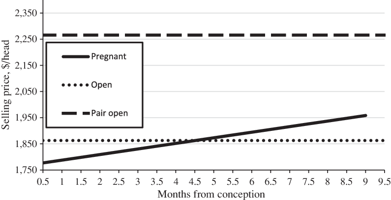
Figure 1. Replacement [breeding] female pregnancy status and cow–calf pair* (source: Marshall et al. (Reference Marshall, Maples, Parish and Coatney2019).
*Assumes the reference categories and mean values of continuous variables.
It appears that the state of pregnancy and length of gestation should be separately controlled for when both pregnant and nonpregnant females are sold. If not, the pregnancy status results will likely depend on the population distribution over months pregnant. For instance, if the data analyzed by Mintert et al. (Reference Mintert, Blair, Schroeder and Brazle1990) or Parcell, Schroeder, and Hiner (Reference Parcell, Schroeder and Hiner1995) consisted primarily of females that are more than 5 or 6 months into pregnancy, then the estimated premium over nonpregnant females would be consistent with the current findings. As reported in Table 1, the average months pregnant in the current data is roughly 3.5 months. To test this hypothesis, months pregnant is deleted from the REM model. The result indicates a significant discount remains of $23.50/head for the average pregnant female.Footnote 15 In all, the initial discount and subsequent increasing value into gestation indicate that the buyers are accounting for risks of abortion increasing/decreasing the earlier/later in gestation, as found in the cited production literature.
5.3. Due Date
The expected calving due date is a new control in BF ICM framework. Pregnant BFs with expected due dates in the summer months (June, July, and August) consistently received significant discounts (average $61.81/head) relative to those expected to calve in March. However, clustered standard error results also include discounts for the months of February and November. Generally, these results are consistent with a priori expectations for preferred calving periods (winter months) in the Southeast. The summer months are not only detrimental to the reproductive success of a BF as cited but also reduces the expected survivability, and hence expected value of the unborn calf.
5.4. Udder and Teat Scores
Two other new variables introduced into BF ICM framework are udder and teat condition. These reproductive success characteristics are expected to be important regarding the BF’s ability to deliver milk to her unborn (if pregnant) and future calves. As expected, as udder condition increased the premiums increased (maximum of $80.37/head) relative to poorer scores of 4 and 5. Unexpectedly, teat condition was not significant, suggesting buyers at auction focus more on udder condition than teats for rearing calves.
5.5. Cow–Calf Pairs
A BF with a calf at her side has proven her reproductive success as to conception, carrying a live calf to term, and birthing. Consistent with Parcell, Schroeder, and Hiner (Reference Parcell, Schroeder and Hiner1995) in sign, the results indicate a significant premium of $462.33/head for an open cow–calf pair over an open BF. The premium indicates buyers are willing to pay the seller to assume a portion of the risk of abortion and dystocia. Given the calf’s weight is unknown in the data (as was the case in Parcell, Schroeder, and Hiner, Reference Parcell, Schroeder and Hiner1995), the buyer’s valuation of reproductive success in regard to the expected value of future calves cannot be separately identified from the NPV of the observed calf at her side.
The value of a nonpregnant (open) cow–calf pair relative to both nonpregnant (open) and pregnant females is portrayed in Figure 1. As can be seen, the value of a BF and who is near term without a calf at her side significantly lags the value of nonpregnant cow–calf pair by roughly $300/head. In support of Parcell, Schroeder, and Hiner (Reference Parcell, Schroeder and Hiner1995) interpretation, the highest valued BF is pregnant, later in gestation, and has a calf at her side ready to wean.
5.6. Body Weight
Consistent with past research (Mintert et al., Reference Mintert, Blair, Schroeder and Brazle1990; Parcell, Schroeder, and Hiner, Reference Parcell, Schroeder and Hiner1995; Pierce and Parcell, Reference Pierce and Parcell1999; Mitchell, Peel, and Brorsen, Reference Mitchell, Peel and Brorsen2018), the impact of body weight on value is positive and experiences decreasing returns. Decreasing returns is indicative of increasing maintenance costs (Bir et al., Reference Bir, DeVuyst, Rolf and Lalman2018). Therefore, the results indicate body weight positively impacts a buyer’s expectation of the net values of the unborn (if pregnant) and future calves, as well as the expected salvage value (Coatney, Shaffer, and Menkhaus, Reference Coatney, Shaffer and Menkhaus2012).
5.7. Body Condition
As expected, compared to an ‘emaciated ‘or ‘extremely thin’ body condition, ‘heavier ‘conditioned BFs received a premium. It was not expected that an ‘excessively over-conditioned’ (score of 7 or combined 8 and 9) BFs would receive an additional premium. The reasoning was based on decrease in the expected reproductive success due to the possibility of dystocia if pregnant, as was also expected for poor conditioning, as well as a signal of infertility if open. However, a plausible reason may be that buyers believe she will produce an unborn calf (if pregnant) and future calves who develop and maintain body condition. Higher conditioning may be a signal to buyers of a greater degree of thriftiness and health, something she will pass on to her calf. Additionally, higher conditioned BFs would be expected to have a higher salvage value if unable to breed back and subsequently sold to packer buyers.
5.8. Frame Size
Medium- and small-framed BFs were similarly priced, while large-framed females were significantly discounted as compared to medium-framed females. This result is likely due to producers realizing the increasing feed costs and lower reproduction rates associated with larger-framed BFs. These negative factors appear to outweigh expectations of increased growth and value potential of the unborn and/or future calves via heredity. The current results are in stark contrast to the premium found for large-framed (primarily slaughter) cows by Parcell, Schroeder, and Hiner (Reference Parcell, Schroeder and Hiner1995). Given the differences in cow types analyzed, however, it cannot be concluded that there has been a shift in producer preferences since 1995.
5.9. Muscling
The lack of significance of muscling score found in Parcell, Schroeder, and Hiner (Reference Parcell, Schroeder and Hiner1995) was not supported in the results. Increases in muscling score were generally found to progressively increase price, relative to a muscling score of 4 (very thin). One notable exception is that clustering standard errors did not find a significant difference between muscling scores 3 (thin) and 4. Therefore, the results indicate that increasing muscling score increases the expected values via improved growth expectations of the unborn calf (if pregnant) and future calves by heredity, and to some degree, the expected salvage value via improved red meat yield.
5.10. Temperament
Another new variable introduced into BF ICM framework is temperament score. Counter to expectations, increases in docility did not systematically increase price, relative to an ‘extremely’ aggressive female. However, ‘moderately’ aggressive females did receive a premium. Although producers do not typically prefer to handle ‘extremely’ aggressive cows, especially with calves by their side, the results suggest buyers value a ‘moderate’ level of aggressiveness. A potential reason is that a ‘moderately’ aggressive female indicates to buyers she possesses the necessary protectiveness to raise her calf, while viewing docility as a lack of thriftiness.
5.11. Locomotion
Locomotion (soundness) is the final new variable introduced into BF ICM framework. As expected, fully ‘sound’ females garnered a premium over those designated as ‘moderate’ to ‘extremely’ lame. The estimated added value is $102.70/head. This result suggests that buyers are aware of asset longevity and the plausible impact of poor locomotion has on the expected number of future calves. Only in the case of clustered standard errors did females with ‘slight’ lameness garner a significant premium of $31.09/head over their lamer counterparts.
5.12. Breed
The results indicate Angus cross, Brangus, Brangus cross, and Brahman cross received significant premiums over Angus BFs ($27.40, $27.79, $95.47, and $93.74/head, respectively). Only in the case of clustered standard errors did Brahman females garner a premium ($91.65/head) over Angus BFs. All other breed types were either not significantly different from Angus (Red Brangus or Red Brangus cross, Beefmaster or Beefmaster cross, Red Angus cross, Simmental or Simmental cross) or received significant discounts (Red Angus, Hereford, Hereford cross, Charolais, Charolais cross, Other Beef, Holstein, Holstein cross (clustered only), and Other Dairy). By and large, Brahman influence and the value it brings in relation to reproductive success in the Deep South is important to Mississippi producers.
5.13. Market Forces: Months Sold, Slaughter Cow Price, and Feeder Cattle Price
Except for February, all other months sold were discounted relative to March. Mississippi BFs follow a similar seasonal pattern to that observed in the Texas cull cow market. Only in the case of clustered standard errors was the month of May not significantly different than March.
Although the expected sign for concurrent average slaughter cow prices follow expectations, the parameter ($76.41/head) is not statistically significant. This result may be due the linkage between two comparable females across the two markets is not adequately defined. For instance, both heavier BFs and slaughter cows are more valuable in both markets, thus a comparable heavier slaughter cow would constitute a more appropriate floor price. Therefore, it may be beneficial in future research to use a matching procedure (e.g., propensity score) to align individual females more closely across the two markets.
The final two market forces results are consistent in sign and significance with the findings of Mitchell, Peel, and Brorsen (Reference Mitchell, Peel and Brorsen2018). First, the results indicate an increase of $75.46/head for each additional $/lb. in feeder calf prices (significant for the HAC methodology only). The results indicate a significant decrease of $337.61/head for each additional $/bushel in corn futures prices.
6. Conclusions and Implications
The primary value of breeding stock is derived from the value of selling offspring. As such, much of the economic literature related to beef cattle valuation has focused on the value of feeder cattle. Less is known about the asset value of dams from which the offspring receive half their genetic potential. Because a minimum objective of beef breeders is to produce a [live] calf, those characteristics of the dam that influence the reproductive success are of major interest for this analysis.
By developing a conceptual characteristics based asset valuation model and discussion of a priori expectations from the economics and production literature, it became apparent that some BF characteristics not only impact the value of offspring via genetic transfer but also reproductive success and expected salvage value (i.e., body condition, body weight, frame size, and muscle thickness). Additionally, some characteristics are related only to reproductive success and discounted expected net returns, such as age and locomotion and their impact on the expected number of future calves; and pregnancy status and its impact on the risk of abortion and expectations of breeding back in the future. Some characteristics are related only to the likelihood that the BF can raise a live calf after birth, such as body, teat, and udder condition. Therefore, asset valuation of dams is complicated and if not estimated properly will result in inefficient asset pricing.
This research builds upon previous BF economics literature (Mintert et al., Reference Mintert, Blair, Schroeder and Brazle1990; Parcell, Schroeder, and Hiner, Reference Parcell, Schroeder and Hiner1995; Mitchell, Peel, and Brorsen, Reference Mitchell, Peel and Brorsen2018) by estimating a hedonic asset characteristics demand model based on individual animals to better understand the influence of reproductive success characteristics. Contrary to previous research (Mintert et al., Reference Mintert, Blair, Schroeder and Brazle1990; Parcell, Schroeder, and Hiner, Reference Parcell, Schroeder and Hiner1995), pregnant BFs do not necessarily receive a premium. It appears Mississippi buyers account for the uncertainty of pregnancy status and discount pregnant BFs compared to nonpregnant females. However, a premium is gained for each additional month in pregnancy, which is consistent with other hedonic research on pregnant BFs (Mintert et al., Reference Mintert, Blair, Schroeder and Brazle1990; Hagerman et al., Reference Hagerman, Thompson, Ham and Johnson2017; Mitchell, Peel, and Brorsen, Reference Mitchell, Peel and Brorsen2018). Interestingly, only those less than 5 months into gestation were discounted relative to nonpregnant females, while those over 5 months into gestation received a premium. Therefore, it appears producers account for the risk of abortion and are not necessarily willing to pay a premium for pregnant BFs as previously thought. Consistent with past research (Parcell, Schroeder, and Hiner, Reference Parcell, Schroeder and Hiner1995), this relationship is enhanced by the relatively large premium found for retaining the BF until she has calved and sold as a pair. As such, it may be the case that previous findings of pregnancy premiums are driven by the distribution of pregnancy term length and not pregnancy status itself. Taken together, these results are indicative of buyers accounting for the risk of abortion for early gestation and the subsequent retention costs, as well as a perceived reduction in production risk of proven females.
The results of this analysis identify implicit net marginal values, the first step in conducting a benefit–cost analysis related to the sales of BFs. Using the empirical results from this analysis in conjunction with Mississippi State University 2019 cow–calf cost budgets, Marshall et al. (Reference Marshall, Maples, Parish and Coatney2019) conducted a benefit–cost analysis of pregnancy checking and market timing of BF. Their research found that sellers of pregnant BFs are made strictly better off financially by absorbing the risk of abortion and dystocia and sell the BF after calving. If nonpregnant, sellers are better off selling immediately. However, Little, Forrest, and Lacy (Reference Little, Forrest and Lacy2000) report that only one-third of the Mississippi cow/calf producers’ pregnancy check occasionally and most never pregnancy check. Therefore, it is beneficial to pregnancy check a potential BF prior to auction as the state and stage of pregnancy negatively impacts sale price relative to selling a cow/calf pair.
Finally, some care must be taken when weighing the magnitudes, and to a lesser degree the significance, of the estimated premiums and discounts found in this study due to the point in time in which the data was collected (2014 to 2015). During the prolonged drought from 2011 to 2013 that impacted numerous states in the south east and south western regions of the United States, a large portion of the cow herd was liquidated. The reduction in the herd size led to shortages in the number of feeder cattle beginning in 2014 leading to higher prices for feeder cattle. At the same time, cow–calf revenues increased dramatically, and potentially the NPV expectations for producers looking to rebuild or expand their herds (fig. 2 in Tonsor and Schulz, Reference Tonsor and Schulz2015,). Mintert (Reference Mintert2019) verified that herd expansion began in 2014 with the first signs of slowing in 2017. Prices for both feeder cattle and replacement cows were reaching their post 2000 peak levels between the last quarter of 2014 and third quarter of 2015 (fig. 2 in Hagerman et al., Reference Hagerman, Thompson, Ham and Johnson2017), the time frame of this study. The dynamics of the cattle market are important in hedonic analysis as it has been shown that marginal implicit value estimates for some feeder cattle quality, value added attributes, and management practices change over time and space due to changes in buyer preferences (Zimmerman et al., Reference Zimmerman, Schroeder, Dhuyvetter, Olson, Stokka, Seeger and Grotelueschen2012; Blank, Saitone, and Sexton, Reference Blank, Saitone and Sexton2016). This could be the case regarding replacement females as well. It is plausible that the bidders in this study were focused more on herd expansion to capture increases in calf values and profits and less concerned with the marginal value product of physical characteristics. If this were the case, then the discount and premium estimates in this study may be smaller than would be expected when buyers are experiencing tight returns where the value of the marginal product of each attribute is more carefully considered in the buyer’s valuation process. To test this proposition, future valuation studies over time and space for replacement females are required.


 Open access