


1 Introduction
Many classes of astronomical objects are known to be variable radio sources, including the Sun, the planets, cool stars, stellar binary systems, neutron stars, supernovae (SNe), gamma-ray bursts (GRBs) and active galactic nuclei (AGNs). There have been extensive studies of these objects using targeted surveys, but few blind, unbiased surveys for variable radio phenomena. An effective survey for radio variability needs to maximise the metric
 \begin{equation}
A \Omega \left(\frac{T}{\Delta t}\right),
\end{equation}
\begin{equation}
A \Omega \left(\frac{T}{\Delta t}\right),
\end{equation}
where A is the effective collecting area of the telescope, Ω is the solid angle coverage of the survey, T is the total duration of the observations, and Δt is the time resolution (Cordes et al. Reference Cordes2004; Cordes Reference Cordes2007). Typically blind radio surveys have had either too small a field of view and too little time coverage per field of view to allow a comprehensive survey for transient and variable phenomena.
The Square Kilometre Array (SKA)Footnote 1 is a proposed future radio telescope (Dewdney et al. Reference Dewdney, Hall, Schilizzi and Lazio2009) that will be many times more sensitive than any existing facility. Should it go ahead, the SKA will be designed to explore five key science projects: galaxy evolution, cosmology, and dark energy; strong-field tests of gravity using pulsars and black holes; the origin and evolution of cosmic magnetism; probing the dark ages—the first black holes and stars; and the cradle of life, searching for life and planets. In addition, there is an awareness of building in (or not designing out) the possibility of serendipitous discoveries. In particular, the dynamic radio sky is recognised as a rich and relatively unexplored discovery space (Cordes et al. Reference Cordes2004; Cordes Reference Cordes2007). Plans for the SKA are still under development, with a Phase 1 instrument expected to be completed in 2020 and a Phase 2 instrument in 2024.
The Australian Square Kilometre Array Pathfinder (ASKAP)Footnote 2 is a precursor and technology development platform for the full SKA and will greatly improve on our ability to detect radio transients and variable sources. Its moderately high sensitivity (RMS of ∼1 mJy beam−1 in 10 s), combined with a wide field of view (covering 30 deg2 of sky in a single pointing), will enable fast, sensitive all-sky surveys (Johnston et al. Reference Johnston2007, Reference Johnston2008). ASKAP is currently under construction in Western Australia. The final telescope will have 36 12-m antennas, with a maximum baseline of 6 km. The wide field of view is enabled by the use of Phased Array Feeds (Chippendale et al. Reference Chippendale, O’Sullivan, Reynolds, Gough, Hayman and Hay2010) of 100 dual-polarisation pixels that will operate over the range 700–1800 MHz. A summary of the planned ASKAP specifications is given in Table 1. The 6-antenna Boolardy Engineering Test Array (BETA) is expected to be completed in late 2012 and will allow some early testing of the techniques required for the full ASKAP surveys.
Table 1. ASKAP Specifications

ASKAP is primarily a survey instrument, and this is reflected in the time allocation policy. In its initial 5 years of operation, 75% of the available time will be scheduled for several major Survey Science ProjectsFootnote 3 that were selected through a competitive call for proposals (Ball Reference Ball2009).
In this paper we describe one of these projects, an ASKAP Survey for Variables and Slow Transients (VAST).Footnote 4 In the context of ASKAP, ‘slow’ means variability or transient behaviour detectable on timescales greater than the cadence on which images will be performed (expected to be 5–10 s). A related project, The Commensal Real-Time ASKAP Fast-Transients Survey (CRAFT; Macquart et al. Reference Macquart2010), will search for ‘fast’ transients on timescales shorter than 5 s. Different techniques are required to process and analyse data for fast and slow transients, and from a scientific perspective this division roughly represents a separation between coherent and incoherent emission processes. The main science goals of VAST are
-
• to detect and monitor ‘orphan’ GRB afterglows to understand their nature;
-
• to conduct an unbiased survey of radio SNe in the local Universe;
-
• to determine the origin and nature of the structures responsible for extreme scattering events (ESEs);
-
• to make a direct detection of baryons in the intergalactic medium;
-
• to discover flaring magnetars, intermittent or deeply nulling radio pulsars, and rotating radio transients through changes in their pulse-averaged emission;
-
• to investigate intrinsic variability of AGNs;
-
• to detect and monitor flare stars, cataclysmic variables, and X-ray binaries (XRBs) in our Galaxy; and
-
• to discover previously unknown classes of objects.
To achieve these goals, VAST will conduct three surveys, in addition to commensal observing with other ASKAP projects: VAST-Wide, aimed at detecting rare, bright events, will survey 10 000 deg2 day−1 to an RMS sensitivity of 0.5 mJy beam−1; VAST-Deep, aimed at detecting unknown source classes, will survey 10 000 deg2 down to an RMS sensitivity of 50 μJy beam−1; and VAST-Galactic which will cover 750 deg2 of the Galactic plane, plus the Large and Small Magellanic Clouds down to an RMS sensitivity of 0.1 mJy beam−1. The full survey parameters are shown in Table 2 and discussed in Section 4.
Table 2. Survey Parameters for the VAST Surveys (see Section 4.1 for Details)

Notes. The two components of the VAST-Deep survey are discussed further in the text. The Commensal column gives an indication of the amount of time that VAST will have access to through commensal observing with other ASKAP projects
In Section 2 we motivate the VAST surveys by discussing the science goals in more detail, and explain how they fit in the context of existing efforts. We also make predictions about the likely source populations that will be observed by VAST. In Section 3 we review previous and current blind radio surveys, as well as archival studies. In Section 4 we describe the proposed VAST survey strategy in detail. Finally, in Section 5, we discuss the design of the VAST transient detection pipeline.
2 VAST Science
Astronomical transient phenomena are diverse in nature, but they can be broadly classified on the basis of their underlying physical mechanism into one of four general categories: explosions, propagation effects, accretion-driven, and magnetic field-driven events. In this section, we discuss the main VAST science goals in each of these areas and discuss the expected populations for different types of sources.
2.1 Explosions
GRBs and SNe are some of the most energetic explosions in the Universe. Although they have been studied extensively there are a number of unresolved questions about their nature, including the existence of radio orphan afterglows (Levinson et al. Reference Levinson, Ofek, Waxman and Gal-Yam2002), the beaming fraction of GRBs (Sari, Piran, & Halpern Reference Sari, Piran and Halpern1999; Dalal, Griest, & Pruet Reference Dalal, Griest and Pruet2002), and the current rate of massive star formation in the Universe as traced by the cosmological radio SN rate. These questions can be addressed by surveys that observe a large area of the sky to good sensitivity, on a regular basis. The capacity of VAST to detect these rare objects is orders of magnitude greater than previous blind surveys such as those of Gal-Yam et al. (Reference Gal-Yam2006) and Bower et al. (Reference Bower2007).
2.1.1 Gamma-Ray Bursts
The afterglow emission from GRBs is generated via particle acceleration in the decelerating blast wave. At late times, the peak of the afterglow spectrum is at radio energies, and thus radio studies provide the most interesting probes for GRBs science. Based on previous studies (Chandra & Frail Reference Chandra and Frail2012), we expect that the GRBs seen by ASKAP will be long-lasting but intrinsically fainter on average than shorter wavelength afterglows. Given the sensitivity of ASKAP, this means that those GRBs studied by VAST will, in general, be the rare but important nearby (∼1 500 Mpc) events. In the relativistic expansion phase (up to 100 d after the initial explosion), ASKAP monitoring in conjunction with optical and X-ray facilities will allow us to measure physical parameters such as the total kinetic energy of the explosion, the density of the circumburst medium, and the geometry of the outflow.
At late times, when the blast wave has decelerated to sub-relativistic velocities, the jetted outflows expand and become more isotropic. Under these circumstances, the total (i.e. calorimetric) energy of GRB blast waves may be estimated—a key but difficult parameter to measure (Frail et al. Reference Frail2005). Instead of relying on rare, nearby events, VAST may also obtain a robust beaming-independent estimates of GRB energies from a large sample of single-epoch flux density measurements (and limits) of afterglows at late times (Shivvers & Berger Reference Shivvers and Berger2011).
As the relativistic beaming is totally suppressed at late time, radio monitoring is the best solution to identify ‘orphan afterglows’, i.e., those GRBs whose jet is beamed away from us (Rhoads Reference Rhoads1997). While they would lack a gamma-ray trigger by definition, such systems could be distinguished from other classes of transients through the evolution and luminosity of their light curves, their location towards galaxies that resemble other GRB hosts, and their probable association with SNe (Soderberg et al. Reference Soderberg2010). The discovery of a population of orphan afterglows would allow us to constrain the beaming fraction of GRBs—a key quantity for understanding the true GRB event rate. It would also open up an order of magnitude more objects which can be scrutinised in detail. This may also give insights on the jet structure of GRBs and clarify the puzzling lack of jet breaks from the Swift satellite (Racusin et al. Reference Racusin2009).
2.1.2 Supernovae
While thermonuclear (Type Ia) SNe have proved to be extremely useful in measuring the acceleration of the Universe, no Type Ia SN has ever been detected at radio wavelengths (Panagia et al. Reference Panagia, Van Dyk, Weiler, Sramek, Stockdale and Murata2006; Hancock, Gaensler, & Murphy Reference Hancock, Gaensler and Murphy2011; Chomiuk et al. Reference Chomiuk2012), indicating a very low density of circumstellar material. In contrast, many core-collapse SNe (those of Type Ib, Ic, and the various Type II sub-classes) have been detected and monitored at radio wavelengths (Weiler et al. Reference Weiler, Panagia, Montes and Sramek2002; Ryder et al. Reference Ryder2004; Soderberg Reference Soderberg, Immler, Weiler and McCray2007). Radio observations replay the late phases of stellar evolution (in reverse), and reveal clues about the late-time evolution of the progenitor system.
With VAST we will conduct an unbiased census of core-collapse SNe (a still undetermined fraction of which emit at radio wavelengths), allowing us to match radio detections against optically discovered SNe. We will also detect new radio SNe that may have gone undetected in the optical or infrared (IR) due to significant amounts of dust (Kankare et al. Reference Kankare2008). The prevalence of such heavily obscured SNe is virtually unconstrained, with hints that they may constitute a nontrivial subpopulation. Recently, SN 2008cs (Kankare et al. Reference Kankare2008) was detected in the IR and confirmed in the radio bands, and SN 2008iz (Brunthaler et al. Reference Brunthaler, Menten, Reid, Henkel, Bower and Falcke2009) was serendipitously discovered in radio observations of M 82. SN 2008iz has remained undetected in the optical, IR, and X-ray bands despite sensitive searches (Brunthaler et al. Reference Brunthaler2010). Discovery of new SNe is valuable for tying down the current rate of massive star formation in the Universe and for understanding how and when SNe explode in star-bursting galaxies. Radio emission from core-collapse SNe is detectable within days, and they reach their peak luminosity at 1.4 GHz as much as 1 year after the explosion, making them ideal targets to detect and study with the sensitivity and cadence of VAST (see Section 4).
Beyond the large population of standard core-collapse SNe, there exist sub-classes of objects that are of particular interest. For instance, radio observations of a recent type Ib/c supernova, SN2009bb, showed that it was expanding at mildly relativistic velocities (β≈0.8) powered by the central engine (Soderberg et al. Reference Soderberg2010). Such SNe are usually associated with GRBs and are discovered by their intense but short-lived gamma-ray energy emission. Yet, SN2009bb had no detected gamma-ray counterpart. It has been suggested that the blast waves produced in such engine-driven SNe could be responsible for the acceleration of ultra-high-energy cosmic rays (Chakraborti et al. Reference Chakraborti, Ray, Soderberg, Loeb and Chandra2011). However, the present limits on the neutrino flux expected as a by-product of cosmic-ray production in GRBs are at least a factor of 3.7 below predictions (Abbasi et al. Reference Abbasi2012). Radio surveys with the capability of completing the sample of these explosions will improve our understanding of particle acceleration processes and the diversity of core-collapse events (see Lien et al. Reference Lien, Chakraborty, Fields and Kemball2011 for predictions on the detection rates of core-collapse radio SNe for a range of SKA pathfinder instruments).
2.1.3 Gravitational Wave Counterparts
Gravitational wave (GW) events are expected to be compact and involve significant energies—both GRBs and SNe are considered to be among likely sources of both electromagnetic and GW emission. In an analogous manner, other classes of GW events may also generate significant transient radio emission, especially if they occur in dense environments. We discuss the particular case of mergers of neutron star binaries in Section 2.3.4. For all classes of GW events, however, localisation will be a significant challenge, with search areas expected to be of the order of 10–100 deg2 for planned GW detectors (Fairhurst Reference Fairhurst2011). The large instantaneous sky coverage of ASKAP makes it particularly valuable in the search for electromagnetic counterparts to GW events, although there are significant uncertainties in the requisite search sensitivities and timescales. The search area estimates mentioned above are computed for the Advanced LIGO (Harry et al. Reference Harry2010) and Advanced VIRGO (Accadia et al. Reference Accadia2011) detectors. These systems are planned to come online in the 2014–2015 timeframe, meaning that ASKAP will be well positioned to make discoveries in this parameter space.
2.2 Propagation
Plasma Propagation Effects: At centimetre wavelengths, any object with an angular size of ≲1 mas is subject to the effects of interstellar scintillation (ISS), caused by inhomogeneities in the ionised interstellar medium (ISM) of our Galaxy. Refractive ISS (RISS) is manifested as slow intensity variations with a wide correlation bandwidth that is caused by large-scale refracting structures in the ISM. Much faster variations that have narrow frequency scales are associated with diffraction from small-scale irregularities (DISS). Observations of the intensity fluctuations caused by ISS can be used to infer both the small-scale structure of the ISM and the structure of a scintillating source on scales down to ∼10-200 mas for compact extragalactic sources and ∼10 nanoarcsec for some pulsars.
The density inhomogeneities in the ionised ISM are typically characterised as a power law (Armstrong, Rickett, & Spangler Reference Armstrong, Rickett and Spangler1995). However, a small number of pulsars have displayed strong fringing events in their dynamic spectra, in which the normal, random appearance of the dynamic spectrum caused by DISS is modified by the appearance of quasi-periodic fringes. Both pulsars and AGNs have displayed ESEs in their light curves, in which their flux densities exhibit marked decreases (≈50%) bracketed by modest increases; and a number of AGNs have exhibited intra-day variability (IDV), marked by flux density variations on timescales of hours. Fringing events are interpreted most naturally as the beating of two distinct images of the pulsar and both ESEs and IDV can be interpreted as due to lensing events through a plasma. All of these phenomena could occur if there is a temporary increase in the amount of power on scales of the order of 1013 cm along or close to the line of sight, e.g., as due to a discrete ‘cloud’ of electrons drifting in front of the pulsar or AGN (Cordes & Wolszczan Reference Cordes and Wolszczan1986; Clegg, Fey, & Lazio Reference Clegg, Fey and Lazio1998). In the case of IDV, it may also be the case that transient, high brightness temperature structures are required to be produced in the cores of some AGNs.
The characteristics of the discrete structures inferred to be responsible for these phenomena are such (density >100 cm−3 and temperature >103 K) that they would be highly overpressured with respect to the bulk properties of the ISM (Kulkarni & Heiles Reference Kulkarni, Heiles, Kellermann and Verschuur1988), and would likely be transient structures. While there is some evidence to suggest that a small fraction of the volume of the ISM is at a high pressure (Jenkins & Tripp Reference Jenkins and Tripp2001), the distribution of such highly overpressured structures is not known, although the characteristics of IDV in some AGNs suggest that some structures are extremely close to the Sun (∼1-10 pc). The existence of such highly overpressured structures in the local ISM is hard to reconcile with our current understanding of interstellar turbulence (e.g. Fiedler et al. Reference Fiedler1987b; Walker Reference Walker, Haverkorn and Goss2007). Alternatively, these phenomena may indicate that a simple power law is not a good description of the spectrum of density inhomogeneities, which would then constrain the nature of the plasma processes involved in the generation and maintenance of the density inhomogeneities.
Because these propagation events are transient in nature, many of the previous observations have been ‘accidental’, happening to catch a source displaying such an event during the course of observations designed for other reasons. There have been relatively few surveys designed specifically to try to find propagation events, with notable examples being the Green Bank Interferometer (GBI) monitoring program (Fielder et al. Reference Fielder, Dennison, Johnston, Waltman and Simon1994; Lazio et al. Reference Lazio, Waltman, Ghigo, Fiedler, Foster and Johnston2001b) and the Micro-Arcsecond Scintillation-Induced Variability (MASIV) survey (Lovell et al. Reference Lovell2003, Reference Lovell2008). Moreover, because of either limited sensitivity, limited field of view, or both, most surveys have only been able to monitor a relatively small number (∼100) of relatively strong sources (≳100 mJy).
A wide-area, high cadence, sensitive survey would be able to place strong constraints on both the spatial distribution of the structures responsible for propagation events and the likelihood of a source exhibiting such an event. In turn, these much stronger constraints can be used to infer properties of the ionised ISM and the mechanisms by which such structures are generated. As an illustration of the kind of monitoring program that ASKAP will enable, a survey could be designed to produce daily flux density measurements of sources stronger than about 10 mJy with the capability to detect 50% flux density changes at the 10σ level. At this sensitivity level, a survey of even only 1 000 deg2 would still be able to monitor nearly compact 50 000 sources.
Gravitational Lensing: Aside from the plasma propagation effects discussed in more detail below, we also note that strong gravitational lensing of active galaxies by galaxy clusters can lead to an achromatic time-domain signal that contains information about both the active galaxy and the intervening space–time. Radio observations of strong lensing have been conducted successfully with existing facilities and those data have been used to constrain cosmological parameters (e.g. Fassnacht et al. Reference Fassnacht, Pearson, Readhead, Browne, Koopmans, Myers and Wilkinson1999; Myers et al. Reference Myers2003). These operate by spatially separating the lensed components of the active galaxy. In general ASKAP will not have the angular resolution to observe such multiple imaging, but the large number of sources monitored with regular cadence means that an autocorrelation analysis (as performed by Barnacka, Glicenstein, & Moudden Reference Barnacka, Glicenstein and Moudden2011) can itself constrain lens time delays.
2.2.1 Pulse Broadening from Scattering
The well known temporal broadening of pulsar pulses caused by scattering from electron-density variations will affect any source of short-duration bursts, including those that will be targeted by VAST. Pulse broadening from sources in the Galactic centre can be broader than 1 000 s at 1 GHz. Bursts from extragalactic sources at cosmological distances can similarly be broadened, especially if the line of sight intersects another galaxy but also from the intergalactic medium (IGM). Scattering in the Milky Way, in other galaxies, and in the IGM therefore define pulse-broadening horizons beyond which pulses with specific widths will not be seen (see e.g. Cordes Reference Cordes2012). Pulse broadening from scattering can be distinguished from source-intrinsic effects by identifying across the ASKAP band the strong frequency dependence ∼∝ν−4 of scatter broadening.
2.2.2 Extreme Scattering Events
ESEs are flux density variations marked by decreases in flux density bracketed by increases (Figure 1). There is widespread agreement that ESEs are caused by refractive lens-like density perturbations along the line of sight to a background source (e.g. Fiedler et al. Reference Fiedler1987b; Romani, Blandford, & Cordes Reference Romani, Blandford and Cordes1987). The refracting lenses which cause ESEs must be Galactic in origin and probably lie within a few kpc, but in the 24 years since their discovery, no satisfactory physical model has emerged for the ESE phenomenon. An analysis of existing data suggests that ESEs are unlike any other identified component of the ISM and that they are present in vast numbers in the Galaxy (with a density ∼103 pc−3). If the refracting properties are taken at face value, they imply regions with pressures ∼1 000 times higher than the diffuse ionised ISM. One suggestion is that they are associated with neutral, self-gravitating gas clouds (Walker Reference Walker, Haverkorn and Goss2007), in which case they would make a substantial contribution to the total baryonic mass content of the Galaxy. Alternatively, they may represent small-scale density enhancements created by converging flows in a turbulent medium (Jenkins & Tripp Reference Jenkins and Tripp2001), but it is unclear whether such structures could persist for the observed ESE durations.

Figure 1. An extreme scattering event in Q0954+658 at 2.7 GHz (lower) and 8.1 GHz (upper) adapted from Fiedler et al. (Reference Fiedler1987b). For clarity, an offset of 1 Jy has been added to the top trace. The strong frequency dependence of ESEs and the necessity of regular sampling of the light curves over a long period is evident. At ASKAP frequencies (∼1 GHz), the amplitude of the flux density decrease would likely have been even larger, and the flux density would likely have increased to an even higher value during the start of the event.
A wide-area survey with daily cadence would allow us to address the physical composition and origin of the objects responsible for ESEs in a comprehensive manner.
Population statistics: One of the more comprehensive ESE surveys (Fiedler et al. Reference Fiedler1994b) provided a total coverage of approximately 600 source-years; VAST has the potential to achieve a coverage that is larger by a factor of roughly 300, searching for ESEs towards sources with much lower flux densities. In turn, an increased coverage will constrain the spatial density and distribution of refracting lenses in the Galaxy, including whether they are associated with particular Galactic structures (Fiedler et al. Reference Fiedler, Pauls, Johnston and Dennison1994a). A larger number of ESEs will also allow investigation into any potential diversity in light-curve shapes, and whether any such diversity can be understood in terms of simple models (Clegg et al. Reference Clegg, Fey and Lazio1998) or the extent to which more complex models of the density structures, background sources, or both, are required.
Real-time characterisation of ESEs: A straightforward approach to elucidating the nature of the structures responsible for ESEs would be to conduct additional observations of a source while it is undergoing an ESE. Events like those seen towards quasars B0954+658 and B1749+096 (Fiedler et al. Reference Fiedler1994b) or B1741−038 (Fiedler et al. Reference Fiedler, Johnston, Waltman and Ghigo1992; Clegg, Fey, & Fiedler, Reference Clegg, Fey and Fiedler1996) should be seen at the rate of roughly 60 per year in an all-sky monitoring survey with ∼1 mJy RMS sensitivity, with ∼10 in progress at any given moment. Thus, in contrast to the GBI monitoring program, for which only one ESE was identified while it was ongoing, VAST will enable real-time follow-up.
Some key follow-up measurements could be made at higher frequencies, particularly in the optical to X-ray bands, which should directly reveal the dense neutral gas clouds responsible for ESEs via scattering, absorption and refraction (Draine Reference Draine1998). Additionally, H i observations would reveal any associated neutral structures, Faraday rotation measurements may constrain the magnetic field strength within the structures, and high-resolution observations could confirm predicted changes in the apparent structure of the source. While there have been previous efforts in conducting such observations (Clegg et al. Reference Clegg, Fey and Fiedler1996; Lazio et al. Reference Lazio2000, Reference Lazio, Gaume, Claussen, Fey, Fiedler and Johnston2001a), only one source has been observed in such a manner (B1741−038), and, for some of the measurements, only a single observation during the actual ESE could be obtained. An all-sky survey could detect multiple ESEs during the course of a year, allowing ample opportunity to trigger follow-up observations with other telescopes and at other wavelengths.
2.2.3 Interstellar Scintillation of AGNs
Observations of decimetre variability in extragalactic sources (e.g. Hunstead Reference Hunstead1972) led quickly to the recognition that the sources needed to have extremely compact components, be affected by interstellar scintillation, or both (Armstrong, Spangler, & Hardee Reference Armstrong, Spangler and Hardee1977; Spangler et al. Reference Spangler, Fanti, Gregorini and Padrielli1989). The need for extremely compact components, apparently violating the so-called inverse Compton catastrophe, became even more acute with the discovery of ‘flickering’ (Heeschen Reference Heeschen1984), and later intra-day variability.
The MASIV 5-GHz Very Large Array (VLA) survey (Lovell et al. Reference Lovell2003, Reference Lovell2008) and other observations (Kedziora-Chudczer et al. Reference Kedziora-Chudczer1997; Dennett-Thorpe & de Bruyn Reference Dennett-Thorpe and de Bruyn2002; Bignall et al. Reference Bignall2003, Reference Bignall, Macquart, Jauncey, Lovell, Tzioumis and Kedziora-Chudczer2006) have established that the fast—intra-day and inter-day—flux density variations at centimetre wavelengths exhibited by a subset of compact quasars are predominantly caused by ISS rather than intrinsic variability. Intra-day variability refers to sources whose characteristic timescale is less than 24 h, while inter-day variability refers to sources whose timescale exceeds this.
Scintillating AGNs are of astrophysical interest because the small angular sizes that they must possess in order to exhibit rapid ISS require brightness temperatures near, or possibly in excess of, the 1012 K inverse Compton limit for incoherent synchrotron radiation. In several cases over the past decade, it appeared that the Doppler boosting factors required in order to reconcile the apparent brightness temperature with the inverse Compton limit were well in excess of the typical values determined from Very Long Baseline interferometric observations of quasars. Estimates of the Doppler boosting factors are subject to considerable uncertainty related to the distance of the scattering material from the Earth, but many of the most rapid IDVs appear to require Doppler factors of a few tens (Macquart et al. Reference Macquart, Kedziora-Chudczer, Rayner and Jauncey2000; Rickett, Kedziora-Chudczer, & Jauncey Reference Rickett, Kedziora-Chudczer and Jauncey2002; Bignall et al. Reference Bignall, Macquart, Jauncey, Lovell, Tzioumis and Kedziora-Chudczer2006; Macquart & de Bruyn Reference Macquart and de Bruyn2007).
More recently, it appears that the fastest manifestations of IDV are associated with sources whose lines of sight intersect more local, albeit much more inhomogeneous, patches of turbulence than previously supposed. Thus, there has been a transfer of our ignorance away from the physics of the AGN and onto the physics of interstellar turbulence. However, this issue is not yet conclusively resolved, as little is known about the origin (or physical plausibility) of the local, highly inhomogeneous scattering screens that need to be invoked to explain the observed scintillation properties of these sources.
The four-epoch MASIV survey (Lovell et al. Reference Lovell2003, Reference Lovell2008) detected variability in 56% of the 482 sources observed but the characteristics of the variability changed from epoch to epoch. While able to illustrate this ISS intermittency, the MASIV survey itself, because of its limited duration and cadence, could not address many of the resulting questions, notably the extent to which the intermittency results from changes in the ISM properties or changes in the sources. In order to address the cause of the intermittency, a survey must have the following characteristics. It must observe a large number of sources widely distributed on the sky so as to have robust statistics and to be able to search for correlations expected for ISS (e.g. a Galactic latitude dependence or with nearby structures in the ISM). The survey must measure both the total and linear polarisation intensity of the sources—ISM-driven intermittency should result in the linear polarisation scintillation tracking that of the total intensity, while source-driven intermittency should result in the linear polarisation and total intensity scintillating nearly independently of each other. The survey must be conducted with close to daily cadence to capture the scintillation variations, and over a multi-year timescale in order to separate changes in source structure or scattering medium from changes associated with the annual cycle resulting from the Earth's orbital velocity.
In addition to determining the cause of ISS intermittency and mapping the scattering properties of the local ISM, such a survey would address the existence of AGN emission above the inverse Compton brightness limit and potentially constrain the baryonic content of the IGM as a function of redshift.
The cause of ISS intermittency: By continuously observing a large sample of sources over a long period, VAST will comprehensively determine the intermittency properties of scintillating AGNs. It will discriminate between ISM-related and source-driven effects via polarisation variations, as discussed above. A complication arises because annual cycles in the variability timescale (caused by the Earth's velocity vector changing with respect to the scattering screens) need to be distinguished from true IDV intermittency. However, these two phenomena can be separated by making regular (daily) observations over the course of at least 2 years. The variations should be dissimilar between epochs separated by a year if the scintillation is intermittent. Intermittency, if caused by the ISM, points to the physical nature of the turbulent patches responsible for IDV.
AGN emission above the inverse Compton brightness limit: In some cases, fast scintillation may be attributable to the appearance of microarcsecond structure within a source, associated with an outburst (Macquart & de Bruyn Reference Macquart and de Bruyn2007). The rise and fade times of the manifestation of fast variations allow us to determine the longevity of microarcsecond components associated with IDV. The rate at which the AGN supplies energy to power the bright emission that causes the variability, and the rate at which energy losses cause its eventual decay. These rates can then be compared with specific AGN processes to identify the mechanism associated with the super-Compton radio emission.
Baryonic content of the intergalactic medium: The MASIV survey showed that few sources above z∼2 are variable (Lovell et al. Reference Lovell2008). If this apparent suppression of ISS as a function of source redshift is confirmed by VAST, there are a number of possible explanations: (1) intrinsic source evolution; (2) gravitational microlensing; or (3) scattering in the turbulent ionised IGM. If the last is at least partially responsible, then the angular broadening is caused by the cumulative effect of all the baryons in the ionised IGM. The sheer number of sources VAST can monitor will enable us to probe in detail the evolution of structure in the ionised IGM as a function of redshift.
One potential complication with scintillation studies is that the largest amplitude IDV is typically observed at frequencies near 5 GHz. At ASKAP frequencies, it is possible that the strength of scattering, even towards high Galactic latitudes, and intrinsic source diameters will result in large-amplitude scintillations being quenched (Dennison & Condon Reference Dennison and Condon1981), although lower amplitude refractive scintillations may still be exhibited (e.g. Dennison et al. Reference Dennison1987).
2.3 Accretion and Magnetism
Along with explosions and propagation effects, accretion and magnetic fields are frequently implicated in transient events. Accretion onto a compact object is a powerful energy source that drives both local sources such as XRBs and microquasars as well as extragalactic blazars and AGNs at cosmological distances. The accretion flow is often connected to an outflow in the shape of a jet, which is the source of the radio emission. The intimate link between the accretion disc and the jet is demonstrated by the fundamental plane of black hole activity that describes a correlation between the mass of the black hole, the jet power, and the accretion power (Merloni, Heinz, & di Matteo Reference Merloni, Heinz and Matteo2003; Falcke, Körding, & Markoff Reference Falcke, Körding and Markoff2004) in AGNs. This relation can be extended to lighter black holes where it matches the correlation between the X-ray and radio luminosities in XRB black hole candidates (BHCs) that was found by Gallo, Fender, & Pooley (Reference Gallo, Fender and Pooley2003). Radio emission is also observed from XRBs containing weakly magnetised neutron stars, such as Z and atoll sources, although they are at least one order of magnitude fainter in radio than the BHCs (e.g. Fender Reference Fender2006), and a weak radio jet has also been observed from the cataclysmic variable SS Cyg during a dwarf nova outburst (Körding et al. Reference Körding, Rupen, Knigge, Fender, Dhawan, Templeton and Muxlow2008). There is still not a good theoretical understanding of how accretion discs produce outflows, but most models assume that the jet is accelerated by a magnetic field (e.g. Blandford & Payne Reference Blandford and Payne1982). VAST will allow us to characterise the full range of transient jet phenomena across the fundamental plane.
Magnetic fields can also act in other ways. They can convert the rotational energy of their source into electromagnetic energy and the mechanical energy of an outflow, as happens for instance in a radio pulsar, or they can release their own energy in the form of flares on a star or the radio emission from Jupiter and (possibly) Jupiter-like extrasolar planets. With VAST we will be able to reveal the unifying physical principles that underlie such diverse behaviour.
2.3.1 Intrinsic Variability in Active Galactic Nuclei
As discussed in Section 2.2.3, Fiedler et al. (Reference Fiedler1987a) observed a sample of 33 AGNs, with flux densities of a few Janskys, every day for more than 6 years. All sources were variable over this time span with typically smooth variations in flux with quasi-periods of months to years. VAST will produce light curves and detect this sort of variability for more than 104 sources over the whole sky. The Fermi gamma-ray satellite observes the whole sky every 3 h and has detected blazar variability on timescales as short as 6 h (Abdo et al. Reference Abdo2010). Simultaneous measurements of the gamma-ray and radio variability in blazars will provide us with a powerful tool for understanding the physics of the central engines in AGNs.
Beyond single black holes in AGNs, a number of binary supermassive black holes (SMBHs) are known or suspected (e.g. Komossa Reference Komossa2006; Rodriguez et al. Reference Rodriguez, Taylor, Zavala, Peck, Pollack and Romani2006; Smith et al. Reference Smith, Shields, Bonning, McMullen, Rosario and Salviander2010; Burke-Spolaor Reference Burke-Spolaor2010). The evidence for these varies, but it is clear that with the mergers of galaxies the central SMBHs could also merge. The act of inspiralling may lead to radio transients accessible to ASKAP. This is because the SMBHs will likely move through a static magnetic field provided by an accretion disc, and this should drive electromagnetic jets (Palenzuela, Lehner, & Liebling Reference Palenzuela, Lehner and Liebling2010; Lyutikov Reference Lyutikov2011; Moesta et al. Reference Moesta, Alic, Rezzolla, Zanotti and Palenzuela2012). The detailed emission processes are unclear, but it is plausible that there could be a radio signature accessible to ASKAP before (O’Shaughnessy et al. Reference O’Shaughnessy, Kaplan, Sesana and Kamble2011) or during (Kaplan et al. Reference Kaplan, O’Shaughnessy, Sesana and Volonteri2011) the merger. Numerous other electromagnetic mechanisms have also been proposed; see Schnittman (Reference Schnittman2011) for a detailed discussion. Combining the radio observations with observations at other wavelengths or even with GWs would significantly improve our understanding of galaxy mergers (e.g. Sesana et al. Reference Sesana, Gair, Berti and Volonteri2011).
2.3.2 Tidal Disruption Events
Tidal disruption events (TDEs) occur when a star wanders too close to a black hole at the centre of a galaxy or star cluster. The black hole tidal forces tear the star apart, but the debris continue on ballistic orbits around the star and are accreted as they approach periastron on the following orbit. The resulting sudden increase in the black hole accretion rate may be directly detected at optical and X-ray frequencies. After the initial flare up, the luminosity decays as t −5/3 (Rees Reference Rees1990). Several candidates of such TDEs have been detected serendipitously through all-sky X-ray and ultraviolet surveys (Grupe, Thomas, & Leighly Reference Grupe, Thomas and Leighly1999; Komossa & Bade Reference Komossa and Bade1999; Komossa & Greiner Reference Komossa and Greiner1999; Esquej et al. Reference Esquej, Saxton, Freyberg, Read, Altieri, Sanchez-Portal and Hasinger2007, Esquej et al. Reference Esquej2008; Gezari et al. Reference Gezari2006, Reference Gezari2008, Reference Gezari2009, Reference Gezari2012; Lin et al. Reference Lin, Carrasco, Grupe, Webb, Barret and Farrell2011; Cenko et al. Reference Cenko2012a; Saxton et al. Reference Saxton, Soria, Wu and Kuin2012).
Crucially, black hole accretion is often accompanied by relativistic jets, with a mechanical power often comparable to the radiative luminosity. The jet can be a source of beamed radio emission and hard X-rays in a way similar to a blazar. To a hard X-ray telescope such as the Burst Alert Telescope (BAT) on the Swift, it will initially resemble a GRB, but it will be distinguished by its much longer duration. Swift J1644+57 is the first observed example of such a TDE candidate, at a redshift of z=0.35. It was discovered as a luminous X-ray transient and was observed across the electromagnetic spectrum, enabling multi-band analysis and modelling of the event (Bloom et al. Reference Bloom2011; Levan et al. Reference Levan2011; Zauderer et al. Reference Zauderer2011; Berger et al. Reference Berger, Zauderer, Pooley, Soderberg, Sari, Brunthaler and Bietenholz2012; Wiersema et al. Reference Wiersema2012). The mass of the central black hole responsible for this event was derived to be ≲107 M⊙ and the ejecta Lorentz factor ≳10. More recently, another TDE candidate has also been detected by the Swift in hard X-rays, Swift J2058.4+0516 (Cenko et al. Reference Cenko2012b).
The main difference between AGN and TDE jets is that the former propagate to Mpc distances, and create characteristic cocoon/lobe structures where their kinetic power is dissipated. In contrast, TDE jets are impulsive ejections that produce a forward shock/reverse shock structure as they interact with the ISM (Sari & Piran Reference Sari and Piran1995). As there is no pre-existing cavity around the previously quiescent black hole, TDE jets have to propagate through a much denser environment and decelerate to sub-relativistic speed at distances of ≲1 pc. Most of their kinetic power is expected to be dissipated in the reverse shock (Giannios & Metzger Reference Giannios and Metzger2011). Typical TDE radio flares from the disruption of a solar-mass star by a 107 solar mass black hole are expected to peak in brightness after ∼1 year, reaching a flux density of ∼2 mJy at 1.4 GHz, for a distance of 1 Gpc corresponding to z=0.2 (not including the effect of relativistic boosting for jets oriented along our line of sight). At peak brightness, the expected radio spectrum is inverted (self-absorbed) with F ν∼ν−2 below ∼2 GHz, and F ν∼ν−1/3 above that (Giannios & Metzger Reference Giannios and Metzger2011).
Radio afterglows of TDEs would be a powerful tool to understand jet physics and source geometry, through measurement of the flux evolution and polarisation. The expected degree of polarisation for these events is low if they are collimated, similar to GRB afterglows. Recent IR and radio polarisation measurements have been found to be consistent with theoretical expectations (Metzger, Giannios, & Mimica Reference Metzger, Giannios and Mimica2012; Wiersema et al. Reference Wiersema2012).
Radio detections of TDE jets hold the key to other unsolved astrophysical problems (e.g. Krolik & Piran Reference Krolik and Piran2012). It is well known that not all accreting black holes have jets, but it is not clear why. Jets are formed only at certain ranges of accretion rate, but other parameters such as the black hole spin may also be important. Finding what fraction and what type of X-ray-detected TDEs have radio jets will help address this question, and will shed light on the evolution of nuclear black holes in galaxies. Furthermore, the timescale for the formation of a radio-bright TDE jet will help us understand how quickly a collimated magnetic field is generated inside the transient accretion disc.
The predicted brightness of TDEs at gigahertz frequencies suggests that VAST should be able to detect about a dozen events per year. A systematic survey of the radio sky would be able to constrain the rate of TDEs and reduce the collimation uncertainty significantly. In particular, the discovery of an entirely new population of orphan TDEs would allow us to place solid constraints on the occurrence rate of this phenomenon and therefore test the theoretical prediction that we should see ∼10−4 yr−1 per galaxy (Rees Reference Rees1990).
2.3.3 Accreting Neutron Stars, Black Holes and Microquasars
Exploring the connection between accretion discs and jets in XRBs requires correlated radio and X-ray observations (Fender Reference Fender2006). The VAST survey will reveal and subsequently measure the radio emission from a large number of XRBs and allow us to search for new radio outbursts. This, coupled with the recent availability of large field-of-view instruments like Swift-BAT and Fermi- Gamma-ray Burst Monitor (GBM), and with the early results (from 2013) of eROSITA's all-sky survey, will provide a large sample of XRBs with active jets, and will allow us to do statistical studies of their time variability properties and X-ray/radio correlation.
VAST will yield information on the population of XRBs showing quasi-steady-state radio jets, which are mildly relativistic and are associated with non-thermal, radiatively inefficient accretion states (Fender et al. Reference Fender2004; McClintock & Remillard Reference McClintock and Remillard2006). For these persistent jets, fundamental properties such baryonic content, energy budget, emission mechanism, and the role played by the spin of the compact object are not well constrained (Markoff et al. Reference Markoff2005; Narayan Reference Narayan1996; Yuan et al. Reference Yuan2005), and regular radio monitoring will allow us to investigate them. In addition, we will determine the duty cycle of the radio-loud phases and test whether radio state transitions (changes in the kinetic power) are always associated with X-ray transitions (changes in the radiative power). We will also investigate what physical mechanism causes major radio flares and the ejection of highly relativistic, optically thin bullets, often associated with the state transition from the hard/non-thermal to soft/thermal state.
In addition to stellar mass and SMBHs, it is predicted that VAST will detect jets from intermediate-mass black holes (IMBHs) with masses between ∼100 and 1 00 000 M⊙. IMBHs may provide a pathway for the formation of SMBHs (e.g. Ebisuzaki et al. Reference Ebisuzaki2001) and also have important connotations for other areas of astrophysics (e.g. Fornasa & Bertone Reference Fornasa and Bertone2008; Wang et al. Reference Wang, Wang, Xiang, Wang, Hao and Yuan2010), but until recently their existence was highly disputed. The discovery of the object known as HLX-1 located in the galaxy ESO 243−49, with an X-ray luminosity of ∼1 000 times greater than the Eddington limit for a 10-M⊙ black hole, currently provides very strong evidence for the existence of IMBHs (Farrell et al. Reference Farrell, Webb, Barret, Godet and Rodrigues2009), with independent studies constraining the mass to 9 000 M⊙ < M BH < 90 000 M⊙ (Davis et al. Reference Davis, Narayan, Zhu, Barret, Farrell, Godet, Servillat and Webb2011; Servillat et al. Reference Servillat, Farrell, Lin, Godet, Barret and Webb2011; Godet et al. Reference Godet2012; Webb et al. Reference Webb2012). Recently, transient radio emission was detected from HLX-1 following a transition from the low/hard to high/soft spectral states, consistent with the ejection of relativistic jets from an IMBH (Webb et al. Reference Webb2012).
Objects such as HLX1 may be very rare (only one known within 100 Mpc), but there are hundreds of ultraluminous X-ray sources (ULXs; see Feng & Soria Reference Feng and Soria2011 for a recent review) in the local Universe with luminosities exceeding the classical Eddington limit of stellar-mass black holes. Most of them are likely to be explained through other mechanisms such as anisotropic emission and/or super-Eddington accretion, but we cannot rule out that a few of them may be IMBHs. In addition, there may be hundreds of low-state or quiescent IMBHs lurking in the core of globular clusters, in the nuclei of dwarf galaxies, or inside recently merged galaxies that may occasionally become active. The detection of jet emission from these objects would allow us to infer the black hole mass, as the radio and X-ray luminosities are correlated as a function of mass (e.g. Fender Reference Fender2006). Steady jets would be undetectable for all but the closest of these objects. However, transient radio flares have been observed from XRBs associated with jet ejection events with radio luminosities a factor of 10–100 times brighter than the non-flaring radio emission (e.g. Körding, Falcke, & Corbel Reference Körding, Falcke and Corbel2006). Such flares should be detectable by VAST out to distances of ∼5–15 Mpc from 1 000-M⊙ black holes, and out to ∼23–72 Mpc from 10 000-M⊙ black holes (S. A. Farrell, in preparation). Thus, we will be able to survey the local Universe for flaring IMBHs, placing constraints on the number density and therefore testing their validity as a pathway for SMBH formation. Conversely, if ULXs are super-Eddington accretors, the detection of radio emission will prove that even at those extreme accretion rates, a substantial fraction of accretion power can come out as kinetic power, and will improve our understanding of black hole feedback at high accretion rates.
2.3.4 Neutron Star Mergers
The merger of two compact objects (neutron stars) is expected to generate strong GWs (Section 2.1.3) but they will also reveal themselves through electromagnetic radiation. The relativistic, beamed outflows detected from short–hard GRBs are thought to originate from such mergers (e.g. Fong et al. Reference Fong2012). VAST is not expected to fortuitously observe such beamed events. However, merger simulations also show that substantial mass can be ejected from these systems quasi-isotropically and at sub- or trans-relativistic velocities, and with energies of 1049-1050 erg (Piran, Nakar, & Rosswog Reference Piran, Nakar and Rosswog2012).
Consider a mildly relativistic blast wave (β0∼0.8) moving out with an energy of ∼1049 erg into the surrounding medium. The shock wave sweeps the surrounding medium and heats it to relativistic temperatures by converting bulk kinetic energy of the incoming material into thermal energy of the shocked material. The electrons in the shock-heated plasma are accelerated in the post-shock magnetic field to radiate synchrotron radiation. This would eventually be optically thin in the gigahertz regime, peaking on a timescale of about a couple of months when the blast wave starts to decelerate. The optimum waveband for detecting these transients, which are also supposed to be prime sources of GWs, is around gigahertz frequencies (Nakar & Piran Reference Nakar and Piran2011). A merger within 300 Mpc would shine as a radio transient of about 1-mJy brightness at ∼1 GHz (A. Kamble & Kaplan Reference Kamble and Kaplan2013), which would be detectable to the VAST and, potentially, also to Advanced-LIGO. Both the peak flux density and the time to peak are uncertain since we lack accurate estimates of the ejecta velocity and energy, and we expect the circumburst density to vary from 1 to 10−4 cm−3.
Using the ‘best-bet’ neutron star merger detection rates predicted for Advanced LIGO (Abadie et al. Reference Abadie2010), we estimate that up to about half a dozen of these transients should be detectable by ASKAP at any given time, although there are significant uncertainties involved. Piran et al. (Reference Piran, Nakar and Rosswog2012) independently estimate ASKAP's sensitivity to these events and obtain similar results. These are comparable to the rate estimated from observations of short GRBs which have been proposed to originate in similar mergers (Coward et al. Reference Coward2012). Metzger & Berger (Reference Metzger and Berger2012) emphasise the challenges related to uncertain GW event localisations, which are significant. As discussed in Section 2.1.3, the large instantaneous sky coverage of ASKAP may be a significant advantage in this situation.
2.3.5 Flaring and Pulsing Neutron Stars
Of the known neutron stars, the vast majority are pulsars that have been detected through their pulsed radio emission. VAST will not be sensitive to radio pulsations on timescales of ≲1 s, but will instead probe neutron star populations that are not selected in pulsar surveys. We will be sensitive to intermittent or deeply nulling radio pulsars as well as radio pulsars with large variations in their average pulsed flux.
Magnetars will be detectable through their rare flaring events such as the giant flare and expanding radio nebula produced by SGR 1806−20 (Gaensler et al. Reference Gaensler2005; Cameron et al. Reference Cameron2005). In addition, some magnetars are known to turn on as radio sources. For example, XTE J1810−197 was initially detected as a transient radio source (Halpern et al. Reference Halpern2005) before its radio pulsations were identified (Camilo et al. Reference Camilo2006). We may also be able to detect bright intermittent pulses from the enigmatic rotating radio transients (RRATs; McLaughlin et al. Reference McLaughlin2006). VAST will thus reveal a broader census of the Galactic neutron star population than a standard pulsation search, with subsequent implications for the overall SN event rate in our Galaxy.
The radio source FIRST J1023+0038 presents an interesting case study. Initially, it was classified as a Galactic cataclysmic variable (CV; Bond et al. Reference Bond, White, Becker and O’Brien2002) because of its optical spectrum and variability, but its radio flaring behaviour appeared to be anomalous. The classification was called into question because of the changes in the spectrum over time (e.g. Thorstensen & Armstrong Reference Thorstensen and Armstrong2005) and it was eventually re-identified as a transitional object where a recycled radio pulsar had turned on after a low-mass XRB phase (Archibald et al. Reference Archibald2009, Reference Archibald, Kaspi, Bogdanov, Hessels, Stairs, Ransom and McLaughlin2010). The actual transition event had an extremely short duration, with the accretion disc apparently dissipating between 2001 December and 2002 May. The radio pulsar was probably absent in 1998 (upper limits of 1.8 and 3.4 mJy at 1.4 GHz) but detected in a survey in mid-2007 with a flux density of ∼14 mJy at 1.6 GHz.
2.3.6 Classical Novae
Novae occur in binaries (CVs) that consist of a white dwarf that is accreting matter from its companion star. A nova is a thermonuclear explosion in the layer of accreted matter on the surface of a white dwarf. A shell of matter is ejected during the explosion and this shell might produce radio emission. The radio emission can persist for a few years after the explosion, and in the case of FH Ser it reached ∼10 mJy at 2.7 GHz about 1 year after the outburst. In the late stages when the ejecta is optically thin, radio emission is generated by the entire ejecta and can therefore be used to estimate the total ejecta mass (see e.g. Hjellming Reference Hjellming, Cassatella and Viotti1990 for a review).
2.3.7 Flare Stars, Pre-Main-Sequence Stars, and Rotation-Driven Stellar Activity
There are several types of stars that display large flares that can be observed in the radio band. The most common are cool dwarf stars of spectral type M or later including brown dwarfs. The flares have typical flux densities above ∼1 mJy, but there is also quiescent emission at the sub-mJy level between the flares (e.g. Pestalozzi et al. Reference Pestalozzi, Benz, Conway and Güdel2000). For these types of systems, it has been argued that radio observations are the best way to obtain information on the stellar magnetic field strength (Berger Reference Berger2006). The number of flaring events that are potentially detectable is unclear, but Berger (Reference Berger2006) obtained a detection rate of ∼10% for objects of later spectral class than M7. They also find that the radio to X-ray luminosity ratio increases over at least three orders of magnitude for these objects compared to earlier spectral classes. VAST will undertake a census of such stars in the local (10 pc) neighbourhood.
In AM Her-like systems (cataclysmic variables in which the white dwarf has a surface magnetic field of ∼103-104 T), the M dwarfs are forced to corotate with the binary, which has an orbital period of a few hours. The dwarf star then becomes more active; flares in AM Her itself have been observed to be as bright as 10 mJy at 5 GHz (Dulk, Bastian, & Chanmugam Reference Dulk, Bastian and Chanmugam1983).
Another group of stars that can produce radio flares are the RS CVn systems (Gunn et al. Reference Gunn, Spencer, Abdul Aziz, Doyle, Davis and Pavelin1994). These are close detached binaries consisting of two main-sequence or evolved stars of spectral type F or later that are tidally locked. The rapid spin of the stars leads to strong magnetic activity, which is manifested as large spots on the stars and also as flaring activity that can be observed both in X-rays and at radio wavelengths.
Flare-like outbursts are also observed in pre-main-sequence stars, but it is not clear whether the physical mechanism is really that of a stellar flare or related instead to the accretion flow onto the star. Such outbursts have been observed in both naked T Tauri stars, which do not show signs of extended accretion discs, and in systems with an IR excess, which indicates the presence of a disc (Osten & Wolk Reference Osten and Wolk2009).
A magnetic field can convert the rotational energy of a star into an outflow and electromagnetic radiation. The most well-known examples of this are the classical radio pulsars, but a similar phenomenon can arise in less extreme stars. Radio observations have detected two fully circularly polarised radio pulses per spin period from the Ap star CU Vir, which is also spinning down in a way similar to a pulsar (e.g. Trigilio et al. Reference Trigilio, Leto, Umana, Buemi and Leone2008, Reference Trigilio, Leto, Umana, Buemi and Leone2011; Lo et al. Reference Lo2012).
Another example of activity driven by rotation is the white dwarf in the cataclysmic variable AE Aqr. The spin period of the white dwarf is 33 s, so rapid that the white dwarf does not accrete the matter that streams over from the companion K dwarf. Instead, the matter is ejected from the system. AE Aqr can be observed over a wide range of frequencies from X-rays to radio, and pulsed emission is observed at optical and X-rays, but it has not yet been detected at radio wavelengths (De Jager et al. Reference De Jager, Meintjes, O’Donoghue and Robinson1994; Bookbinder & Lamb Reference Bookbinder and Lamb1987; Bastian, Dulk, & Chanmugam Reference Bastian, Dulk and Chanmugam1988).
3 Exploration of the Unknown
The most interesting sources detected by VAST may be those we currently know nothing about. A sensitive wide-area blind survey is ideal for detecting such unknown source classes, but one of the challenges in designing the VAST survey is ensuring that the survey parameters do not unduly bias us against unknown source classes that we would otherwise be sensitive to. For example, daily monitoring of a field for 5 min day−1 makes it less likely that we will detect an object that brightens on hour-long timescales and fades within several hours.
Large-scale blind surveys for radio transients have been performed by a number of groups (e.g. Amy, Large, & Vaughan Reference Amy, Large and Vaughan1989; Katz et al. Reference Katz2003; Matsumura et al. Reference Matsumura2007) over the last few decades. These surveys have been severely limited in their sensitivity, sky coverage, and cadence. In spite of this, they have revealed that the radio sky contains many transient objects, the identities of some of which remain mysterious.
For example, Hyman et al. (Reference Hyman2005) discovered a bursting transient towards the Galactic Centre which lasted for only a few minutes with a flux density in excess of 2 Jy at 330 MHz. Subsequent observations showed that the bursts repeated multiple times with a period of ∼77 min and a burst length of ∼10 min. The identification of this source remains unclear (e.g. Kaplan et al. Reference Kaplan, Hyman, Roy, Bandyopadhyay, Chakrabarty, Kassim, Lazio and Ray2008; Roy et al. Reference Roy, Hyman, Pal, Lazio, Ray and Kassim2010), although similarities with bursts from ultracool dwarfs (Hallinan et al. Reference Hallinan2007) are intriguing. Another example is the well-known Lorimer burst, discovered in an archival search of Parkes pulsar data. Lorimer et al. (Reference Lorimer2007) discovered a single millisecond pulse of extragalactic origin with the astonishing peak flux density of 30 Jy at 1.4 GHz (also see Keane et al. Reference Keane, Kramer, Lyne, Stappers and McLaughlin2011 for a second example). Although the nature of this source has been questioned, and recent work suggests that the burst may be terrestrial (Burke-Spolaor et al. Reference Burke-Spolaor, Bailes, Ekers, Macquart and Crawford2011), these new discoveries illustrate that the parameter space for radio variability has not been fully explored yet (Figure 2).
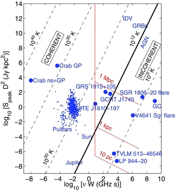
Figure 2. The parameter space for radio transients, adapted from Cordes et al. (Reference Cordes2004). A quantity equivalent to absolute luminosity (observed flux density S multiplied by the square of the distance D 2) is plotted against the dimensionless product of the emission frequency ν and the transient duration or pulse width W. In the Rayleigh–Jeans approximation, these quantities are directly proportional and related to the brightness temperature, as indicated by the diagonal lines, with T=1012 K marking the maximum brightness temperature of incoherent processes. Examples of known radio transient sources are indicated, including giant pulses and ‘nanogiant’ pulses from the Crab pulsar (Hankins et al. Reference Hankins, Kern, Weatherall and Eilek2003), radio pulses from XTE J1810−197 (Camilo et al. Reference Camilo2006), and other pulsars from the Australia Telescope National Facility pulsar catalogue (Manchester et al. Reference Manchester, Hobbs, Teoh and Hobbs2005); the microquasar GRS 1915+105 (Mirabel & Rodríguez Reference Mirabel and Rodríguez1994); radio flares from V4641 Sgr (Hjellming et al. Reference Hjellming2000), the brown dwarf LP 944−20 (Berger et al. Reference Berger2001), and the magnetar SGR 1806−20 (Gaensler et al. Reference Gaensler2005; Cameron et al. Reference Cameron2005); the Galactic centre radio transient J1745−3009 (Hyman et al. Reference Hyman2005); pulses from the ultracool dwarf TVLM 513−46546 (Hallinan et al. Reference Hallinan2007); as well as radio emission from the Sun and Jupiter. Red lines indicate the expected sensitivity of ASKAP to sources at distances of 10 pc, 1 kpc, and 1 Mpc.
In this section, we summarise existing blind and archival surveys for radio transients, focusing on ‘slow’ transients with variability on timescales of seconds or greater.
3.1 Transient Rates from Blind Surveys
Bower et al. (Reference Bower2007) presented the results from an archival survey of VLA data. Since the publication of this work there have been a number of blind radio transient surveys conducted on both archival data and from the first data sets produced by next-generation radio telescopes. Most of these have had the dual aim of (a) searching for individual objects of interest and trying to identify them; and (b) characterising the population statistics of radio transients in order to prepare for future surveys. Although the reported transient rates from Bower et al. (Reference Bower2007) have recently been revised, after a reanalysis of the data by Frail et al. (Reference Frail, Kulkarni, Ofek, Bower and Nakar2012), the work established a framework for comparison of radio transient surveys.
Bower et al. (Reference Bower2007) proposed a metric for comparing the results from blind surveys for radio transients: the two-epoch equivalent snapshot rate, which is equivalent to the transient surface density. Figure 3 shows an updated version of their plot, incorporating a subset of the surveys listed in Table 3 and discussed in the rest of this section. For surveys that made no detection, an upper limit is calculated using a Poisson distribution:
 \begin{equation}
P(n) = {\rm e}^{-\rho A},
\end{equation}
\begin{equation}
P(n) = {\rm e}^{-\rho A},
\end{equation}
where P(n) is the confidence level [i.e. P(n)=0.05 for 95% confidence], ρ is the areal density of transients in a two-epoch survey, equivalent to the snapshot transient rate, and A is the equivalent solid angle, calculated by multiplying the number of images NT by the field of view Ω. We can rearrange Equation (2) in terms of ρ for the purpose of placing theoretical constraints on planned surveys:
 \begin{equation}
\rho = -\frac{\ln P(n)}{\Omega \times N_{T}}.
\end{equation}
\begin{equation}
\rho = -\frac{\ln P(n)}{\Omega \times N_{T}}.
\end{equation}

Figure 3. Log two-epoch snapshot transient rate (deg−2) against log of the flux density (Jy) for surveys that report detections of transient and variables (thick lines). We also include a selection of surveys that report upper limits (thin lines with arrows); see Table 3 for survey acronyms. The surveys are coloured according to frequency: black <1 GHz, blue = 1–4.8 GHz, and red >4.8 GHz (see Table 3 for details). No corrections have been made for spectral index effects. Surveys labelled superscript ‘V’ denote detections of highly variable radio sources; those with superscript ‘T’ denote detections of transient-type sources. The VAST survey predictions are indicated and organised by sub-survey. A description of each survey is given in Section 4. In each case, the vertical segment denotes the RMS that can be achieved per observation. The horizontal segment indicates the upper limit that would be set if no transients or variables were detected in the entire survey. The joining line (between the horizontal and vertical) indicates the upper limits that could be placed by combining data from multiple 5-s snapshots up to the total available integration time per observation (see Table 3). See Section 3.1 for further discussion.
Table 3. Summary of Snapshot Rates for Transient and Variables Radio Sources Reported in the Literature

Notes. The results are organised according to upper limits based on non-detections (top section); transient detections (middle section); and detections of highly variable radio sources (bottom section).
†Note that although Bower et al. (Reference Bower2007) report 10 detections, the reanalysis by Frail et al. (Reference Frail, Kulkarni, Ofek, Bower and Nakar2012) results in only four (uncertain) detections. The snapshot rate calculated by Frail et al. (Reference Frail, Kulkarni, Ofek, Bower and Nakar2012) assumes no detections, and we adopt this as the more conservative position for our analysis.
⋆ Bower et al. (Reference Bower2010, Reference Bower, Whysong, Blair, Croft, Keating, Law, Williams and Wright2011), Bower et al. (Reference Bower, Whysong, Blair, Croft, Keating, Law, Williams and Wright2011), and Bower & Saul (Reference Bower and Saul2011) each state two different rates depending on flux density and timescale; we quote these separately as (A) and (B).
‡See also Bannister et al. (Reference Bannister, Murphy, Gaensler, Hunstead and Chatterjee2011b).
We can improve Equation (3) by taking into account not only the total number of observations in a given survey NT , but the intra-observation cadence τ, out of total observing time per observation T. Doing this results in
 \begin{equation}
\rho = -\frac{\ln P(n)}{\Omega \times N_{T} \times (T/\tau )}.
\end{equation}
\begin{equation}
\rho = -\frac{\ln P(n)}{\Omega \times N_{T} \times (T/\tau )}.
\end{equation}
For example, on the smallest timescale, ASKAP images will be produced every τ=5 s; the total observing time per observation (in one scenario) could be T=1 h and the field could be observed daily for 2 years (NT =730). A 5-s ASKAP image will have an RMS of 1.4 mJy beam−1. If subsequent data or images are stacked together (either via the uv or image plane), the RMS will improve to
 \begin{equation}
\sigma = \frac{1.4 \mbox{ mJy beam}^{-1}}{\sqrt{N_{T} \times (T/\tau )}}.
\end{equation}
\begin{equation}
\sigma = \frac{1.4 \mbox{ mJy beam}^{-1}}{\sqrt{N_{T} \times (T/\tau )}}.
\end{equation}
Equations (4) and (5) have been used to generate survey predictions from the VAST survey parameters described in Section 4, and these predictions are shown in Figure 3. We also include the predicted rates of a subset of known radio transients (see Frail et al. Reference Frail, Kulkarni, Ofek, Bower and Nakar2012, for further discussion). One limitation of the plot in Figure 3 is that it collapses a number of dimensions into a single two-dimensional plot. For example, it does not represent the cadence of the surveys or any trends in transient detection rate with observing frequency.
Surveys typically fall into one of the two categories: many repeated observations of a single field (e.g. Bower et al. Reference Bower2007; Carilli, Ivison, & Frail Reference Carilli, Ivison and Frail2003), or a large area, few-epoch surveys (e.g. Levinson et al. Reference Levinson, Ofek, Waxman and Gal-Yam2002; Gal-Yam et al. Reference Gal-Yam2006). The two-epoch equivalent snapshot rate is a valid metric for quantising the effectiveness of a survey, provided the timescale of transient behaviour is less than the cadence of the observations but longer than a single integration. In this case, a survey with many epochs is equivalent to a larger area survey with two epochs. Further survey metrics have been developed to account for observation cadence and source evolution timescales as well (e.g. Cordes Reference Cordes2007).
3.2 Archival Surveys
The first large radio archival survey of variability and transient behaviour was conducted by Levinson et al. (Reference Levinson, Ofek, Waxman and Gal-Yam2002), who covered a large fraction of the sky with two epochs by comparing the NRAO VLA Sky Survey (NVSS) (Condon et al. Reference Condon, Cotton, Greisen, Yin, Perley, Taylor and Broderick1998) and Faint Images of the Radio Sky at Twenty-Centimeters (FIRST) (White et al. Reference White, Becker, Helfand and Gregg1997) surveys, both at 1.4 GHz. Various corrections were made to account for the different footprint of each survey and their differing resolutions (45 arcsec for NVSS compared to 5 arcsec for FIRST). Nine possible radio transients were reported by Levinson et al. (Reference Levinson, Ofek, Waxman and Gal-Yam2002), but a follow-up of these sources with the VLA by Gal-Yam et al. (Reference Gal-Yam2006) ruled out five of these as false candidates and two as non-variable sources. The effective survey area was 5 990 deg2; hence, with two detections the overall transient snapshot rate was ρ=1.5×10⁻³ deg−2.
Another large area survey was conducted by Bannister et al. (Reference Bannister, Murphy, Gaensler, Hunstead and Chatterjee2011a), using archival data from the Molonglo Observatory Synthesis Telescope (Mills Reference Mills1981) which operates at 843 MHz. This data set had the advantage of a common resolution and comparable sensitivity in each epoch, but like the NVSS–FIRST comparison it had a range of cadences between days and years for each field. Bannister et al. (Reference Bannister, Murphy, Gaensler, Hunstead and Chatterjee2011a, Reference Bannister, Murphy, Gaensler, Hunstead and Chatterjee2011b) detected two transient sources from a survey with a two-epoch equivalent area of 2 776 deg2, giving an overall snapshot rate of ρ=1.5×10⁻³ deg−2 for sources above 14 mJy.
An alternative approach has been to use archival calibrator fields which have many repeated observations but a relatively small field of view. Bell et al. (Reference Bell2011) analysed 5 037 observations of VLA calibrator fields at three frequencies (1.4, 4.8, and 8.4 GHz). The observations ran from 1984 to 2008, with typical gaps between observations of between 4.3 and 45.3 d. No radio transients were detected and they therefore placed an upper limit of ρ<0.032 deg−2 for sources brighter than 8.0 mJy between 1.4 and 8.4 GHz.
Likewise, Bower & Saul (Reference Bower and Saul2011) detected no transients in their analysis of archival observations of 3C 286 from the VLA. Their data set spanned 23 years and included 1 852 epochs at 1.4 GHz. They derive upper limits of ρ<3×10⁻³ deg−2 at 70 mJy for timescales of ∼1 d and ρ<9×10⁻⁴ deg−2 at 3 Jy for timescales of ∼1 min. These results, combined with the Croft et al. (Reference Croft2010) results discussed in Section 3.3 below, currently provide the best limits on the number of slow, bright radio transients.
3.3 Gigahertz Surveys
There have been a number of blind imaging surveys specifically designed to search for transient and highly variable sources. Until recently, these have generally been small-area surveys with many epochs, due to the limited field of view of the telescopes used. Early surveys were motivated by searching for radio counterparts to GRBs and SNe. For example, Frail et al. (Reference Frail1994) observed 15 epochs of a field centred on the location of GRB 940301 with the Dominion Radio Astrophysical Observatory Synthesis Telescope at 1.4 GHz. These observations were taken between 3 and 99 d after the initial event and made no detections, which resulted in an upper limit of 3.5 mJy on any time-variable radio sources.
Carilli et al. (Reference Carilli, Ivison and Frail2003) observed the Lockman Hole region to a sensitivity limit of 100 μJy at 1.4 GHz, with five epochs over a period of 17 months. They found that 2% of the sources within their sample were highly variable (defined as ΔS ≥ 50%) and hence derived a rate of ρ=18 deg−2. Also in search of highly variable radio sources, Becker et al. (Reference Becker, Helfand, White and Proctor2010) surveyed the Galactic plane and found ρ=1.6 deg−2 above a sensitivity of 1 mJy at 4.8 GHz. At low Galactic latitude and sampling a multitude of timescales (days to years), Ofek et al. (Reference Ofek, Frail, Breslauer, Kulkarni, Chandra, Gal-Yam, Kasliwal and Gehrels2011) used the VLA to study transient and variables in a field covering 2.66 deg2 to a sensitivity limit of ∼100 μJy at 5 GHz. One transient candidate was reported and a thorough discussion of the variable radio sources within the field was given.
Matsumura et al. (Reference Matsumura2009) summarise the detections of nine candidate transient sources from the Nasu 1.4-GHz wide-field survey (see Kuniyoshi et al. Reference Kuniyoshi2007; Matsumura et al. Reference Matsumura2007; Niinuma et al. Reference Niinuma2007, Reference Niinuma2009; Kida et al. Reference Kida2008, for full details). The sources were detected in a drift scan mode and have flux densities greater than 1 Jy, with typical timescales of minutes to days. (Note, however, the questions raised about these results by Croft et al. Reference Croft2010, Reference Croft, Bower, Keating, Law, Whysong, Williams and Wright2011, and the discussion about the resulting transient event rates by Ofek et al. Reference Ofek, Frail, Breslauer, Kulkarni, Chandra, Gal-Yam, Kasliwal and Gehrels2011.)
As briefly discussed earlier in Section 3.1, Bower et al. (Reference Bower2007) reported the detection of 10 transient radio sources in archival VLA data at 4.8 and 8.4 GHz. Frail et al. (Reference Frail, Kulkarni, Ofek, Bower and Nakar2012) recently reanalysed this data set and reported that more than half of these transients were either caused by rare data reduction artefacts or that the detections had a lower signal-to-noise ratio (S/N) after re-reduction. The Bower et al. (Reference Bower2007) study initially predicted a rate of events over the whole sky of ρ∼ 1.5 deg−2, which is diminished to potentially an order of magnitude less, depending on how the lower S/N level transients are interpreted. For Figure 3, we have adopted the conservative snapshot rate calculated by Frail et al. (Reference Frail, Kulkarni, Ofek, Bower and Nakar2012), which assumes no detections. See Frail et al. (Reference Frail, Kulkarni, Ofek, Bower and Nakar2012) for further discussion.
The Allen Telescope Array (ATA; Welch et al. Reference Welch2009) is the first of the next-generation telescopes to have been used for large-area transient surveys. The Pi GHz Sky Survey (PiGSS) survey was carried out on the ATA at 3.1 GHz and covered 10 000 deg2 of the sky with a minimum of two epochs for each field with an RMS sensitivity of ∼1 mJy (Bower et al. Reference Bower2010).
The first data release (PiGSS-I) is a 10-deg2 region in the Boötes constellation, with 75 daily observations over a 4-month period. Bower et al. (Reference Bower2010) identify one object present in PiGSS that is not in archival radio catalogues (NVSS and Westerbork Northern Sky Survey (WENSS)). From this they set an upper limit on the snapshot rate of transients of ρ<1 deg−2 at 1 mJy sensitivity at 3.1 GHz. The second data release (PiGSS-II; Bower et al. Reference Bower, Whysong, Blair, Croft, Keating, Law, Williams and Wright2011) focused on studying the daily and monthly transient and variable nature of the field. The upper limits of ρ<0.025 deg−2 at 15 mJy for 1-d timescales and ρ<0.18 deg−2 at 5 mJy for 1-month timescales were placed on the rates of transient events at 3.1 GHz.
The other major ATA survey is the Allen Telescope Array Twenty-Centimeter Survey (ATATS; Croft et al. Reference Croft2010), a 690 deg2 survey with 12 epochs of each field. Croft et al. (Reference Croft2010) presented results from comparing a single combined ATATS image with the NVSS. They did not detect any transients, placing an upper limit of ρ<0.004 deg−2 on the transient rate for sources with flux greater than 40 mJy at 1.4 GHz. Croft et al. (Reference Croft, Bower, Keating, Law, Whysong, Williams and Wright2011) extended this analysis presenting results for an individual epoch-to-epoch comparison for the ATATS data set. They derived a limit of ρ<6×10⁻⁴ deg−2 for transients brighter than 350 mJy at 1.4 GHz.
3.4 Low-Frequency Surveys
Since many significant discoveries of radio transients have been made at low frequencies, the low-frequency SKA pathfinders have enormous discovery potential.
The largest blind survey for slow transients at low frequencies was conducted by Lazio et al. (Reference Lazio2010) with the Long Wavelength Demonstrator Array (LWDA). The LWDA is a 16-dipole phased array with all-sky imaging capabilities, operating at 73.8 MHz. A total of 106 h of data (with a typical integration time of 5 min) were searched for transients. No detections were made above a flux density limit of 500 Jy. Lazio et al. (Reference Lazio2010) quote an upper limit on the rate of 1×10⁻² yr−1 deg−1 which converts to a rate of ρ<9.5×10⁻⁸ deg−2 assuming 5-min integrations.
In comparison, one of the deepest low-frequency studies to date has been conducted by Jaeger et al. (Reference Jaeger, Hyman, Kassim and Lazio2012). They used six VLA observations centred on the Spitzer Wide-Area Infrared Extragalactic Survey (SWIRE) Lockman Field at 325 MHz to study sources brighter than 0.2 mJy within a field of view of 6.5 deg2. The timescales of observation ranged from 1 d to 3 months. One transient was reported and the authors argue that it is most likely coherent emission from a stellar flare. Using this detection, Jaeger et al. (Reference Jaeger, Hyman, Kassim and Lazio2012) set an upper limit on the snapshot rate of ρ<0.12 deg−2 for sources brighter than 2.1 mJy at 325 MHz.
Between the two comprehensive low-frequency transient surveys discussed above (Lazio et al. Reference Lazio2010 and Jaeger et al. Reference Jaeger, Hyman, Kassim and Lazio2012) lies a large amount of parameter space both in frequency and time to explore. This will be made possible by two new instruments: the Murchison Widefield Array (MWA; Lonsdale et al. Reference Lonsdale2009; Tingay et al. Reference Tingay2012) and the Low Frequency Array (LOFAR; Heald et al. Reference Heald2011), both currently being constructed and commissioned.
4 Survey Strategy
The detection and characterisation of radio transients requires both the sampling of new regions of parameter space and the ability to monitor and follow up known or newly detected sources. As such, a successful transient instrument requires a large field of view, rapid survey capabilities, high sensitivity and dynamic range, as well as sufficient angular resolution for unambiguous source identification and follow-up. ASKAP will fulfil these criteria with its ability to achieve sub-millijansky sensitivity across the entire visible sky in a single day of observing.
Sources that vary on rapid timescales are necessarily compact. The 10-arcsec resolution of ASKAP will permit source localisation to ∼arcsecond positional accuracy, enabling follow-up observations at other wave bands.
The key to the efficient detection and monitoring of transient and variable sources is the repeated observation of each field to sample a full range of cadences corresponding to the natural timescales of variability in the underlying source population. In addition to observing commensally with other ASKAP programs, we will run a campaign of complementary surveys designed to achieve our science goals. The VAST surveys build on the standard ASKAP imaging pipeline and thus do not include other possible modes of operation such as ‘Fly's Eye' monitoring (e.g. Siemion et al. Reference Siemion2012).
4.1 VAST Surveys
In this section, we outline our strategy for each of the VAST surveys given in Table 2. We have based this survey strategy on an estimate of ∼8 500 h of observing time over the first 5 years of ASKAP operations, in addition to continuous commensal observing with other ASKAP projects. The survey parameters are summarised in Table 2. All of the dedicated (non-commensal) VAST surveys will be conducted with an observing frequency range of 1 130–1 430 MHz.
4.1.1 VAST Wide
To detect rare events such as GRBs and SNe, and to map out the gas density distribution of the ISM across the whole sky, a large survey area is required. To fully sample the ESE light curves, a regular (preferably daily) cadence is desirable. Two years of data are required to discriminate between an annual cycle and intrinsic variability for IDV sources.
Hence, our planned survey will cover 10 000 deg2 (comprised of 400 pointings, each of 30 deg2). Integrating for 40-s per pointing will give an expected RMS sensitivity of 0.5 mJy beam−1, with a total observing time (including overheads) of 6 h day−1. This survey will be repeated daily for 2 years, with a total time of 4 380 h. Figure 3 shows that it will be a substantial improvement over existing blind gigahertz surveys.
4.1.2 VAST Deep
In our Deep survey we plan to observe 10 000 deg2, with 400 pointings each observed for 1 h. This would achieve an expected RMS sensitivity of 50 μJy beam−1. Each of the fields will be observed by the Evolutionary Map of the Universe (EMU) collaboration (see Section 4.2) for their continuum survey (Norris et al. Reference Norris2011). While both the Deep and the Wide surveys observe the same amount of the sky, they are complementary in cadence and sensitivity.
One field, coinciding with a field observed by the EMU collaboration, will be repeated daily for 1 year (Deep Single field). The other fields will be repeated eight times at irregularly spaced intervals (Deep Multi-field). This is the optimal survey to detect as-yet unknown source classes (see Bower et al. Reference Bower2007) and detect GRBs and SNe to larger distances.
4.1.3 VAST Galactic
A third component of VAST is a survey of 750 deg2 of the Galactic plane. This is a total of 30 pointings, plus an additional three pointings, to cover the Large and Small Magellanic Clouds. Each pointing will be observed for 16 min, achieving an expected RMS sensitivity of 0.1 mJy beam−1. The Galactic plane survey will require 9 h of observing in a single day, repeated weekly for 1 year and supplemented by additional epochs at longer intervals.
4.2 Commensal Observing
In addition to the planned surveys, we will operate our transient detection pipeline commensally on all other ASKAP observations. Two projects, EMU (The Evolutionary Map of the Universe; Norris et al. Reference Norris2011)Footnote 5 and WALLABY (The ASKAP HI All-Sky Survey; Koribalski Reference Koribalski2012),Footnote 6 are particularly relevant as they will conduct extensive (possibly commensal) wide-field surveys.
-
EMU: A deep (10μJy beam−1 RMS) survey of the entire Southern Hemisphere, to a declination of δ=+30°.
-
WALLABY: A survey of neutral hydrogen covering two-thirds of the sky to a redshift of z=0.5.
These projects plan to operate in ‘point and shoot’ mode, covering some region of the sky with significant integration time (∼12 h) per pointing and no revisits. This provides an excellent opportunity for detection and monitoring of transient and variable behaviour on timescales of less than a day.
4.3 VAST Predictions
In Figure 3 we show the predictions parameterised via the method described in Section 3, using the VAST survey parameters given in Table 3. Note that the horizontal lines show the upper limits that would be placed if no transient or variable sources were detected. The vertical lines show the RMS that would be expected for the final integration time per image (see RMS sensitivity in Table 3). For the commensal survey, the best RMS is found after 6 h (not 12), assuming that two back-to-back 6-h images are needed to search for transients, i.e., that there are no repeat observations. It can be seen from Figure 3 that the VAST surveys make orders of magnitude improvements on previous surveys.
VAST-Wide will use 4 320 h of dedicated observing time, which is the greatest of all the VAST sub-surveys (excluding commensal observing). It will observe 10 000 deg2 for 40 s every day for 2 years, possibly longer. Observing for 40 s with ASKAP yields an RMS of ∼0.5 mJy beam−1 and produces eight 5-s images per observation. This is represented in Figure 3 and it casts VAST-Wide as less competitive than, for example, VAST-Deep (both multi-field and single field). The limits shown in Figure 3 for VAST-Wide however do not include upper limits on the rate and RMS calculations via combining data from multiple days’ observing.
For example, all the 40-s images taken daily for an entire week could be combined together and compared and searched for transients with the combined images from the next week, and so on. If technically feasible, such an approach will significantly increase the competitiveness of the VAST-Wide survey. Figure 3 also does not convey how many known radio sources will be monitored in each case. VAST-Wide will monitor all known sources in the Southern Hemisphere above 2.5 mJy (5σ) every day for 2 years, whereas VAST-Deep (one field) will monitor only a subset (30 deg2) to a greater sensitivity of 250 μJy (5σ). We can approximate the ratio of sources that will be observed with VAST-Deep (N Deep) to VAST-Wide (N Wide) using the following expression (assuming a Euclidean source population):
 \begin{equation}
\frac{N_{\rm Deep}}{N_{\rm Wide}} = \frac{A_{\rm Deep}}{A_{\rm Wide}} \times \left(\frac{\sigma _{\rm Deep}}{\sigma _{\rm Wide}}\right)^{-1.5} \simeq 10\%,
\end{equation}
\begin{equation}
\frac{N_{\rm Deep}}{N_{\rm Wide}} = \frac{A_{\rm Deep}}{A_{\rm Wide}} \times \left(\frac{\sigma _{\rm Deep}}{\sigma _{\rm Wide}}\right)^{-1.5} \simeq 10\%,
\end{equation}
where in this example A Deep is the survey area of VAST-Deep (single field, 30 deg2) and A Wide is the area of VAST-Wide (10 000 deg2). Here, σDeep and σWide represent the survey sensitivities, respectively. VAST-Wide will therefore monitor large numbers of bright transients and variables, such as IDVs and AGNs. VAST-Deep will be better optimised for studying the faint end of the transient and variable population.
5 Data Processing
The success of VAST hinges on our ability to detect transient sources on the timescales on which images are produced by ASKAP, at the same time as monitoring known variable sources that are in our field. First, how to effectively deal with the large volumes of data and, second, how to find the ‘needles in a haystack’—the most interesting transient sources. As discussed in Section 3, current blind surveys at 1.4 GHz suggest that less than 0.5% of sources observed by VAST will be transient or highly variable (Bannister et al. Reference Bannister, Murphy, Gaensler, Hunstead and Chatterjee2011a).
The operation of the ASKAP data pipeline is described in the Science Processing Document (Cornwell et al. Reference Cornwell2012). The following sections address some of the issues most relevant to VAST and discuss the design and operation of the VAST transient detection pipeline. The overall functionality of the VAST pipeline is illustrated in Figure 4 and described in Table 4. A discussion of the pipeline design is also provided by Banyer et al. (Reference Banyer2011).

Figure 4. Illustration of the VAST pipeline functionality. A description of each stage is given in Table 4.
Table 4. VAST Image Products
5.1 Data Rates
ASKAP is designed to be a real-time telescope, with most of the data processing done in online mode. Data from the phased array feed elements in each antenna will be sent to the beam former to create primary beams. The primary beams from each antenna are sent to the correlator to create visibility data. These data are then sent to the central processor for processing into science-ready data products: images and spectral cubes. The data rate from the correlator to the central processor is expected to be 2.5 GB s−1, generating about 200 TB of raw data every 24 h.
The central processor will operate three data processing pipelines in parallel: one pipeline will produce data cubes designed for spectral line analysis, with high frequency resolution; the second pipeline will produce data cubes designed for continuum surveys, with full polarisation and higher angular resolution, but reduced spectral resolution; the third pipeline is the transient detection pipeline which will produce data cubes with lower frequency resolution, but operating on 5-s timescales (see Table 5). Each 5-s image cube will be up to 16 GB (depending on the number of frequency channels generated and stored), which means that the transients pipeline will process around 12 TB of data an hour. Retaining some coarse frequency resolution will enable post-correlation rejection of radio frequency interference (see Section 5.3) and also provide some minimal spectral information for detected transient sources.
Table 5. Functionality of the VAST Pipeline Components, As Illustrated in Figure 4

5.2 Transient Detection Approach
Source detection is central to all upcoming radio transient surveys, and also those in other wave bands such as the Large Synoptic Survey Telescope transients survey. In the image domain, transient source detection has typically followed one of two approaches: image subtraction or catalogue-based detection.
SN search projects and other optical astronomy projects have typically used the image subtraction approach (e.g. Riess et al. Reference Riess2004; Alcock et al. Reference Alcock2000). In its simplest form, this involves subtracting the current image from some higher sensitivity master image. In practice, some corrections are required, for example each image can be convolved with a kernel to account for coordinate shifts and distortions (Alard & Lupton Reference Alard and Lupton1998; Alard Reference Alard2000).
In radio images, the incomplete u-v coverage means that image subtraction often results in artefacts that can then be mistakenly identified as transient sources. A more robust approach is to first extract and measure sources in each image, and then search for transients by catalogue cross-matching and light-curve analysis. The approach taken in the VAST transient detection pipeline is based on techniques described by Bannister et al. (Reference Bannister, Murphy, Gaensler, Hunstead and Chatterjee2011a), developed for analysing the Molonglo Observatory Synthesis Telescope archive. This is also similar to the approaches taken in the ATA transient projects (Croft et al. Reference Croft2010, Reference Croft, Bower, Keating, Law, Whysong, Williams and Wright2011) and the LOFAR transient detection pipeline (Swinbank Reference Swinbank2007).
We are also investigating the technique of transient detection in the visibility domain (Trott et al. Reference Trott, Wayth, Macquart and Tingay2011; Law & Bower Reference Law and Bower2012). These approaches have the advantage of dealing with well-behaved noise properties of visibilities and avoiding artefacts caused by the imaging and deconvolution processes. Trott et al. (Reference Trott, Wayth, Macquart and Tingay2011) use statistical decision theory to derive detection limits of visibilities using models of the source and calibration effects of interferometers. Law & Bower (Reference Law and Bower2012) present a computationally simple, calibration-independent algorithm for transient detection based on the bispectrum, an interferometric closure quantity. By subtracting visibilities in time, the bispectrum can be used to quantify the significance of transients throughout the field of view. Visibility-based algorithms have great potential in the study of transients, because they take advantage of a priori information to reduce computational burden. This makes real-time processing easier, which may be a critical limitation of the large, computationally demanding surveys described here. More work is needed to understand how these algorithms work on a large scale and whether they can be implemented for real-time analysis.
5.3 Rejection of Radio Frequency Interference
One of the most significant challenges for all radio telescopes is the impact of radio frequency interference (RFI) from man-made sources. Although the ASKAP site was chosen for its radio-quiet properties, signals from satellites used for communications, navigation, remote sensing, and the military pervade all areas of the Earth. Similarly, aircraft communication signals are present even in very remote areas. In addition, self-generated RFI is a challenge as faster digital equipment is used in the signal pathways. There is no universal method of RFI mitigation that is satisfactory for all types of observing techniques and RFI signals (Fridman & Baan Reference Fridman and Baan2001; Briggs & Kocz Reference Briggs and Kocz2005). For the data rates expected with VAST, an automated approach with a combination of techniques will be essential.
RFI mitigation techniques range in sophistication from simple blanking of corrupted data to adaptive cancellation based on coherent detection. Simple blanking works well for strong short-duration RFI, but is completely ineffective in removing low-level time-variable RFI that could mimic transient sources. Blanking removes signal as well as interference and reduces the sensitivity achieved in a given time. There is a growing literature on more sophisticated ideas for RFI elimination. Some of the techniques that we are exploring for VAST include the following.
-
1. Post-detection flagging based on the recognition of data that are affected by interference. This has been the traditional approach in radio interferometry and is appropriate for moderately strong interference, but it does come with a loss of sensitivity.
-
2. Adaptive cancellation techniques such as those described in Mitchell, Robertson, & Sault (Reference Mitchell, Robertson and Sault2005), Briggs & Kocz (Reference Briggs and Kocz2005), and Kesteven et al. (Reference Kesteven, Manchester, Brown and Hampson2010). These require a separate reference antenna or beam on the sky to sample the RFI. An algorithm is used that adapts filter characteristics to match the RFI spectral footprint. This approach requires a high-sensitivity copy of the interferer.
-
3. Spatial filtering techniques that use the location of the known interferer or the relative arrival times of the signals to identify and separate the RFI signal from the astronomical signal (e.g. Leshem, van der Veen, & Boonstra Reference Leshem, van der Veen and Boonstra2000; Ellingson & Hampson Reference Ellingson and Hampson2002; Smolders & Hampson Reference Smolders and Hampson2002; Kocz, Briggs, & Reynolds Reference Kocz, Briggs and Reynolds2010). These are appropriate for stationary or slowly moving RFI sources and require less sensitivity to the interfering source than the adaptive cancellation techniques.
-
4. Adaptive nulling techniques, which employ the capacity of the array to place response nulls on the RFI source. These are appropriate for very strong interfering sources and for telescopes such as ASKAP with independently steerable beams.
-
5. Post-correlation filtering techniques use software algorithms to remove RFI from interferometric data by subtraction of a weak, persistent RFI signal (Athreya Reference Athreya2009) or by implementation of low-pass time and frequency filters to remove variable RFI (Offringa, de Bruyn, & Zaroubi Reference Offringa, de Bruyn and Zaroubi2012). The advantage of these techniques is that they generally have a lower sensitivity requirement for detecting the interference. However, radio interferometers may not be able to use this approach to mitigate some types of slowly varying RFI signals.
5.4 Source Detection
Finding and characterising sources in each of the observed images are critical first steps for transient detection in the image domain. False positives in source finding have the ability to confound the detection of transients, reducing the confidence with which a transient can be detected. This has been identified as a problem in previous surveys, with source-finding errors contributing to the false detection rate (FDR; see, for example, Bannister et al. Reference Bannister, Murphy, Gaensler, Hunstead and Chatterjee2011a; Croft et al. Reference Croft, Bower, Keating, Law, Whysong, Williams and Wright2011; Frail et al. Reference Frail, Kulkarni, Ofek, Bower and Nakar2012).
The source-finding packages that are currently available (for example, the miriad package sfind; Hopkins et al. Reference Hopkins, Miller, Connolly, Genovese, Nichol and Wasserman2002, and the aips package vsad; Condon et al. Reference Condon, Cotton, Greisen, Yin, Perley, Taylor and Broderick1998) are all able to achieve a high degree of completeness and reliability, typically better than 95% on standard radio continuum images. These packages have been extensively used in large-scale radio surveys. However, even a small number of missed real sources, or false positives, can cause problems in the identification of variable and transient sources.
In recent surveys, the best source-finding results have been obtained by using the above-mentioned source-finding packages in conjunction with a pipeline of other programs (see, for example, Mauch et al. Reference Mauch, Murphy, Buttery, Curran, Hunstead, Piestrzynski, Robertson and Sadler2003; Norris et al. Reference Norris2006; Murphy et al. Reference Murphy, Mauch, Green, Hunstead, Piestrzynska, Kels and Sztajer2007). The refinement of the source-finding pipeline is often done after all observations have been completed and the idiosyncrasies of the data are well understood. A lot of time and effort is spent normalising the input images and filtering the resulting catalogues. In many cases, a subset of the final source catalogue is validated ‘by eye’ to ensure that the brighter sources are correctly represented. This approach produces high-quality catalogues and is well suited to single-epoch surveys, as is evidenced by the high level of completeness and reliability that these surveys are able to obtain.
For VAST, the volume of data will require a fully automated source-finding process. The inability to archive every image that is observed for VAST will require that the source finding is done in real-time and without the possibility of reprocessing. The large number of sources that are expected for a single day's observation means that even with completeness and reliability of 99%, a source-finding algorithm will be finding up to ∼10 000 false detections and missing up to ∼10 000 real sources each day. These false detections and missed sources far outweigh the number of true transient and variable sources that we expect to detect.
As part of the VAST design study process, Hancock et al. (Reference Hancock, Murphy, Gaensler, Hopkins and Curran2012) have undertaken a detailed analysis of some of the most widely used source-finding packages in astronomy, including the newly developed selavy (Whiting Reference Whiting2012) and aegean (Hancock et al. Reference Hancock, Murphy, Gaensler, Hopkins and Curran2012) algorithms. For compact sources, we find that the task of source finding (distinguishing between source and background pixels) is a solved problem that the various programs all achieve equally well. However, the task of source characterisation (measuring the various parameters of the found sources) is only accomplished well in the case of single isolated sources. For diffuse sources, the task of source finding is equally well achieved; however, the task of source characterisation is not well defined. Hales et al. (Reference Hales, Murphy, Curran, Middelberg, Gaensler and Norris2012) address some of the issues of extended source measurement. However, since we expect transient sources to be compact, this is not a significant issue for VAST.
Figures 5 and 6 show the FDR and completeness of each of the source-finding algorithms. The FDR and completeness were measured by injecting a known population of sources into a simulated image and processing this image with each of the different source-finding algorithms. A comparison between the input and output catalogues resulted in a set of sources common to both (real detections), a set of sources in the input but not the output (non-detections), and a set of sources that were in the output but not the input (false detections). The set of falsely detected sources consisted entirely of sources within an island of pixels that contains multiple components. These sources were so poorly characterised that they were not able to be linked to a source within the input catalogue. Sources that are poorly characterised also reduce the catalogue completeness. In Figures 5 and 6, the main reason that the source-finding algorithms have non-zero FDR and less than ideal completeness is due to poor source characterisation, rather than poor source finding. In order to better characterise islands of pixels that contain more than a single component, the aegean program analyses the curvature of an image. As can be seen in Figures 5 and 6, aegean is able to characterise islands of pixels that contain multiple components better than any of the other source finding approaches, typically achieving a completeness of over 99.9%. Further details of the source-finding analysis and the operation of the aegean source-finding algorithm are presented by Hancock et al. (Reference Hancock, Murphy, Gaensler, Hopkins and Curran2012).

Figure 5. The FDR for each of the source-finding algorithms (from Hancock et al. Reference Hancock, Murphy, Gaensler, Hopkins and Curran2012). No falsely detected sources are expected above an S/N of 5 for the area of the sky simulated. The non-zero rate of false detections is due to poor source characterisation.

Figure 6. The completeness of each catalogue (from Hancock et al. Reference Hancock, Murphy, Gaensler, Hopkins and Curran2012) as compared to the input catalogue. The coloured curves represent the completeness of the named source finders. The black dotted curve represents the expected completeness of an ideal source finder. The plateau in completeness above and an S/N of 10 is due to sources that are poorly characterised.
5.5 Classification of Transients
Given the large number of sources that we will likely detect with VAST, prompt classification will be critical for early identification and multi-wavelength follow-up. This is a challenging problem due to the sparsity and heterogeneity of the available data. There are two sets of information that can be used for this task: the light curve itself, and the existing archival information about that source or location on the sky.
Light-curve classification has been successfully used to classify variable stars at optical wavelengths (e.g. Richards et al. Reference Richards2011, Reference Richards, Starr, Miller, Bloom, Butler, Brink and Crellin-Quick2012). In order to explore the feasibility of the light-curve classification for VAST, we used several approaches.
First, we simulated light curves of five transient source types: SNe, RS CVn flare stars (fStar_RSCVn), M-class flare stars (fStar_dMe), XRBs, novae; two variable source types: IDVs and ESEs and a non-varying background (BG) for comparison (K. K. Lo et al., in preparation). We experimented with light-curve classification on the simulated light curves in two scenarios:
-
• archival classification, where the classification is performed after a significant amount of light-curve data have been collected; and
-
• online classification, which is the classification of partial light curves in real-time for the purpose of triggering appropriate follow-up observations.
Second, we used light curves from the Palomar-Quest and Catalina Real-Time Transient Surveys to experiment further with a range of machine-learning methods. The results of these experiments are discussed in the sections below.
5.5.1 Archival Classification
We approached the classification problem using the standard methodology of supervised machine learning with 10-fold cross-validation. First, we extracted a set of features from each light curve. These include time-domain features which are simply the flux measurements at each time point (tme), statistical features (stat) such as the mean, standard deviation, and skew, following Richards et al. (Reference Richards2011); statistical (stat) features built cumulatively (stat-cum) after observing a fixed number of observations in multiples of k (k, 2k, etc.); periodic features derived from the Lomb–Scargle periodogram (lsp); and wavelet features derived from the Haar wavelet (wlet). We then created two more feature sets that are concatenations of the above. Feature set all-reps is the concatenation of stat-cum, lsp, and wlet, and feature set all concatenates tme, stat-cum, lsp, and wlet. Details of all seven feature sets are discussed by Rebbapragada et al. (Reference Rebbapragada, Lo, Wagstaff, Reed and Murphy2012).
We used these features as input to a set of machine-learning algorithms, which, when given a training set of examples, will learn the discriminative features for each source type. Using the Weka toolkit (Hall et al. Reference Hall, Frank, Holmes, Pfahringer, Reutemann and Witten2009), we experimented with three classification algorithms: Support Vector Machines (SVM; Cortes & Vapnik Reference Cortes and Vapnik1995), Random Forests (Breiman Reference Breiman2001), and the J48 Decision Tree (Quinlan Reference Quinlan1986). Figure 7 shows the classification accuracy in the archival setting. The Random Forest is the best performing classifier when used with the combined feature sets, achieving 93% accuracy. This suggests that archival classification using light curves alone is feasible with a reasonable degree of accuracy, given the large number of sources. However, the performance on real light curves is likely to be lower since our simulated light curves have ideal Gaussian noise and are aligned to the starting time of the event.

Figure 7. Comparison of overall classification performance (accuracy percentage) by feature set (tme, stat, stat-cum, wlet, lsp, all-reps, and all) and classification algorithm (J48, Random Forest, and SVM), with results grouped by classification algorithm.
5.5.2 Online Classification
The aim of online classification is to identify sources of interest as soon as possible after new observations arrive. The earlier a classification is made, the more likely that a follow-up observation can be scheduled, and so online classification should run continuously as part of the real-time transient detection pipeline. We evaluated online classification using the first 30 d of simulated light curves. With so few observations, it is not possible to extract periodogram or wavelet features; hence, we were limited to the statistical feature set and the time-series values themselves.
Figure 8 shows the confusion matrix for our best performing algorithm: the J48 classifier built with stat features extracted from 30 d of observations. The overall classification accuracy achieved was 50% across eight source types. This is better than the baseline expected from random classification (12% accuracy) but probably not sufficient to be useful in scheduling follow-up observations. Accuracy was improved by grouping source types with similar light-curve characteristics together (grouping SNe and novae, BG, and ESE yielded an accuracy of 70%). Finally, accumulating more data led to higher accuracy (∼80% accuracy with 100 d of observations).

Figure 8. Online classification confusion matrix shown as a heat map (red = higher accuracy, blue = lower accuracy). The x-axis is the classified output class and the y-axis is the actual input class. We used 200 sources of each type and the number in each cell represents how these sources are classified. Overall accuracy at 30 d is 50%.
5.5.3 Other Machine-Learning Approaches
Considerable insight into the classification problem can be gained from the current efforts on classification of transients in optical synoptic sky surveys (Bloom et al. Reference Bloom, Starr, Butler, Nugent, Rischard, Eads and Poznanski2008; Donalek et al. Reference Donalek, Mahabal, Djorgovski, Marney, Drake, Glikman, Graham and Williams2008; Mahabal et al. Reference Mahabal2008a, Reference Mahabal and Bailer-Jones2008b, Reference Mahabal, Djorgovski, Donalek, Drake, Graham, Williams, Moghaddam, Turmon, Mizumoto, Morita and Ohishi2010, Reference Mahabal2011; Djorgovski et al. Reference Djorgovski2011). We experimented with several approaches, using the data from the Palomar-Quest and Catalina Real-Time Transient Surveys, as well as selected data sets from the literature.
Similar to the work described in Section 5.5.1, we parameterised observed optical light curves as feature vectors and applied various machine-learning techniques (e.g. decision trees) to their classification. A set of decision trees was trained using the feature vectors for various combinations of classes. To reduce the dimensionality of the input space, we applied a forward feature selection strategy that consisted of selecting a subset of features from the training set that best predicts the test data by sequentially selecting features until there is no improvement in prediction. Each tree was built using the Gini diversity index as criterion for choosing the split; the splitting stopped when there is no further gain that can be made. To avoid over-fitting we used a 10-fold cross-validation approach. The decision trees were pruned in order to choose the simplest one within one standard error of the minimum. When tested on a data set consisting of light curves of blazars, cataclysmic variables, and RR Lyrae stars, we achieved completeness in the range of ∼83%–97% and contamination in the range of ∼4%–13% (C. Donalek et al., in preparation). In future work, we will apply this to the classification of radio light curves.
Another approach we experimented with used two-dimensional distributions of magnitude changes for different time baselines for all possible epoch pairs in the data set (Djorgovski et al. Reference Djorgovski2011; B. Moghaddam et al., in preparation). These two-dimensional (Δm, Δt) histograms can be viewed as probabilistic structure functions for the light curves of different types. Template distributions for different kinds of transients and variables are constructed using the reliably classified data with the same survey cadences, S/N, etc. For any newly detected variable or a transient, corresponding (Δm, Δt) histograms are accumulated as the new data arrive, and we used a variety of metrics to compute the effective probabilistic distances from different templates. Initial testing indicates that we can obtain a high classification accuracy using this approach. We plan to generalise it to include triplets or even higher order sets of data points for multi-dimensional histograms.
One important lesson so far is that existing archival and contextual data will play a critical role in classification. This includes a spatial context (i.e., what is near the observed event on the sky—a possible host galaxy, a cluster, an SN remnant, etc.), the multi-wavelength context (has it been detected at other wavelengths, what is its broad spectral energy distribution), and the temporal context (what was its flux variability or a detection history in the previously obtained data). Some of this information can be readily extracted from the archives (e.g. flux measurements from different wavelengths, light curves at that location), but some—spatial context in particular—require a human judgement, e.g., is the apparent proximity to other objects (galaxies, clusters, etc.) likely to be relevant, and if so, what does it imply about the transient? Human inspection of vast numbers of transients does not scale to the massive data streams such as those contemplated here. We are currently experimenting with crowdsourcing approaches to harvesting of the relevant human pattern recognition skills and domain expertise, and their translation to machine-processable algorithms.
5.6 Alerts and Follow-up
ASKAP policy specifies that all data and results must be released as soon as they have passed scientific quality control. This is particularly important for transient detections, in which multi-wavelength follow-up is critical. VAST will generate publicly available data products on the following timescales:
-
Seconds: Triggers for individual transient events will be released through services such as VOEventNetFootnote 7 as soon as they are detected. These events will have quality flags representing our confidence about the detection and will allow immediate follow-up of new discoveries by the wider community.
-
Minutes: Triggers with value-added data such as classifications based on multi-wavelength archival cross-matching will be released as soon as our source classification pipeline has run.
-
Days: Measurements of every source in every field will be entered into our light-curve database in near real-time. This will be available immediately to the VAST collaboration. Once quality control has been completed, updates to the database will be made publicly available.
-
Months: Scientific quality catalogues will be constructed from our light-curve database. The results will be published and data made public as soon as possible after analysis is complete.
The quality control process for alerts will consist of a multi-tiered system in which there is automatic filtering of a large fraction of false detections followed by manual inspection of the remaining sources. This approach is taken by several existing transients surveys, for example in the Palomar Transients Factory (Gal-Yam et al. Reference Gal-Yam2011). The detailed implementation of this general approach will be developed and refined during commissioning.
In addition, all images from VAST will be made available through the standard ASKAP archive. Where possible, the VAST pipeline will use standard Virtual Observatory protocols such as VOEvents.Footnote 8
5.6.1 Very Long Baseline Interferometry
As noted earlier, radio sources that are highly variable on short timescales are necessarily intrinsically compact. ASKAP's angular resolution of ∼10 arcsec will be high enough to localise variable sources on the sky and measure variability, but will be orders of magnitude too low to resolve the evolving structures that give rise to the variations in integrated flux. In order to resolve the structure and evolution of the radio source, much higher angular resolution imaging is required, provided by Very Long Baseline Interferometry (VLBI).
Alerts from the VAST pipelines will be used to trigger observations using the Australian Long Baseline Array (LBA), now including telescopes from Western Australia (ASKAP) to New Zealand (Warkworth), allowing milliarcsecond-scale imaging. Due to the very large number of VAST alerts, targets for VLBI follow-up will have to be chosen selectively and will need to be restricted to the most interesting or rare classes of transient and variable sources. The Australian LBA is very well suited to this type of follow-up, as evidenced by previous program that have taken triggers for transient radio sources from Molonglo Observatory Synthesis Telescope (MOST) or the Australia Telescope Compact Array (ATCA) (Tingay et al. Reference Tingay1995; Miller-Jones et al. Reference Miller-Jones2012).
The current LBA has a sensitivity of 60 μJy beam−1 for a 1-h integration at 2.3 and 8 GHz. This is comparable to the sensitivity of ASKAP at 1.4 GHz. With ASKAP incorporated as an element of the LBA, the sensitivity at 1.6 GHz would be 40 μJy beam−1 for a 1-h integration. Hence, a 12-h observation with the LBA would be able to detect any unresolved source found by the VAST surveys.
The recent advent of real-time eVLBI on the LBA means that the VLBI observations can be rapidly processed and analysed. Thus, subsequent observations can be adapted based on the initial results. This facility will benefit studies of new transients that will be detected by ASKAP.
6 Conclusions
Next-generation radio telescopes such as the EVLA, LOFAR, MWA, and ASKAP will have a substantial impact on our ability to discover and monitor radio transient and variable sources. The VAST survey will play an important role in the study of a range of phenomena, from GRB afterglows and SNe through to cataclysmic variables and radio flare stars, as well as propagation effects in the ISM.
The three VAST surveys (VAST-Wide, VAST-Deep, and VAST-Galactic) will allow us to do a comprehensive search of radio transient parameter space. It is likely that in addition to discovering a large number of known classes of objects, we will also discover new types of transient and variable phenomena. Our automatic transient detection pipeline will be able to run simultaneously with other major ASKAP observing projects, meaning that we will also analyse data in commensal mode.
All data products produced by VAST will be released to the wider community as soon as possible after passing quality control standards. Wherever possible, this will be done through the use of Virtual Observatory tools and protocols.
In this paper, we have summarised the science goals of VAST, described our current results in algorithm development for source-finding and transient light-curve classification, and made predictions about the likely source populations that will be observed by VAST.
Acknowledgments
We would like to acknowledge the additional contributors to the optical transient classification work, including Ashish Mahabal, Ciro Donalek, Matthew Graham, Baback Moghaddam, Mike Turmon, and a number of Caltech students. We would also like to thank Peter Ashwell and Andrew Naoum at the University of Sydney for useful discussions. We acknowledge the contribution of the wider VAST collaboration team members through their participation in the design study over the last three years.
This research has been supported in part by the Australian Research Council (ARC). TM, BMG, PJH, JB, and MEB acknowledge support through grants FS100100033 and DP110102034, and through the Science Leveraging Fund of the New South Wales Office for Science and Medical Research. SAF is the recipient of an ARC Postdoctoral Fellowship, DP110102889. TM, BMG, and S. Croft acknowledge funding from the University of Sydney International Program Development Fund. The Centre for All-sky Astrophysics is an Australian Research Council Centre of Excellence, funded by grant CE110001020.
S. Chatterjee acknowledges support from the US National Science Foundation (NSF) through the award AST-1008213. DLK was partially supported by NSF awards AST-1008353 and AST-0908884. SGD acknowledges partial support from the NSF grants AST-0407448, AST-0909182, and IIS-1118041, and the National Aeronautics and Space Administration (NASA) grant 08-AISR08-0085. IHS is supported by an NSERC Discovery Grant. A portion of this research was carried out at the Jet Propulsion Laboratory, California Institute of Technology, under a contract with NASA. US Government sponsorship is acknowledged.


