


INTRODUCTION
Recent studies on the theory and experimental verification of frost heaving have yielded important information. During the freezing of soil, the water in soil migrates to the freezing front. Several proposals to explain the driving forces of this migration have been made. The first explanation drew on a model based on capillarity (Everett I961) according to which the capillary pressure is given For an unsaturated, unfrozen soil as follows:
where Pa is the pressure in the air phase, Pw is the pressure inside water, δua is the surface tension of air-water, and rwa is the effective pore radius of the soil. Such a difference in pressure between water and ice at their interface pulls water toward the interface. Below the layer of the interface it forms a hydraulic pressure gradient. Water migrates along it toward the interface, forming a “freezing front” (Chalmers and Jackson 1970).
By generalizing the Clapeyron equation, Edlefsen and Anderson (1943) defined another model concerning the suction of water in frozen soil. This concept treated the flow of water to the freezing front similarly as did the first model.
It is a well-known fact that when soil freezes, not all of its water freezes simultaneously (Anderson and Morgenstern 1973), and that the amount of unfrozen water in the frozen soil decreases with the lowering of temperature. Thus, if a temperature gradient exists in a frozen layer, the unfrozen water inside frozen soil differs in chemical potential from that inside unfrozen soil. Under this condition, differentiated chemical potential may be defined as differentiated pore-water pressure. Then, it is likely that water flows to the lower side of pore-water pressure.
Generalized and called the concept of coupled heat and moisture transfer in soil during freezing, this third proposal has been tested recently in a variety of attempts to explain water transport, which is the dominant process in frost heaving (Guymon and Luthin 1974; Taylor and Luthin 1976, 1978; Jame and Norum 1980; Sheppard, Kay and Loch 1978). However, as seen from the results, there has been no adequate verification of the model based on this concept.
A mathematical model for simulating heat and water flow in freezing soil was attempted by the present author (Fukuda 1982). Although some interesting numerical analyses were made, few experimental results were obtained to verify the model.
Recently Konrod and Morgenstern (1981, 1982a, 1982b) proposed a new concept called the segregation potential for frost heaving process, modifying the third concept. According to their concept, an ice lens grows somewhere inside frozen soil, slightly behind the freezing front, the warmest isotherm at which ice can exist in the soil pores. The growth of the ice lens depends mainly upon the temperature gradient close to the segregated ice lenses. In the simplest form of the model, water transport to an ice lens might be expressed as follows:
where SP is the segregation potential (mm/s.°C), grad T is the temperature gradient adjacent to the growing ice lens (°C/mm), and v is the velocity of water (mm/s).
In the present paper, the authors attempted to verify this model and apply it to the prediction of field frost heaving.
FIELD OBSERVATIONS OF FROST HEAVE
For the studies of frost heaving, a field site was selected in the Tomakomai Experimental Forest, Hokkaido. A concrete waterproof basin (5 x 5 m wide, 2 m deep) was controlled artificially so that a sufficient amount of water was supplied to the soil to cause a large frost heaving to occur.
Daily changes were recorded in air temperature soil temperature at every 10 cm depth, heave amount of the ground surface and the depth of ground freeze. Heat flow sensors were installed at various depths along with tensiometers within the soil layers. Core samples were removed from the frozen ground several times throughout the experimental period, and their water contents and densities were measured.
A neutron-scattering method was developed by the authors for non-destructive measurement of soil moisture For the neutron source, Californium-252 (252Cf), with an intensity of 100 μCi, which has an effective half-life of 2.64 years and decays by spontaneous neutron emission was used. Emitted fast neutrons with an energy level of 2.38 Mev were scattered by hydrogen atoms, which constitute the soil moisture. Fast neutrons reduce the energy level to 0.025 ev during the process of scattering The intensity of the scattered neutrons (thermal neutrons) was detected by an 3He detector and measured as a count ratio. The system diagram is shown in Figure 1.
If the water content value adjacent to the neutron source is high, high counts of scattered neutrons are obtained. The water content profile was obtained in every 5 cm thick layer in the soil during the process ?f freezing. The typical water content profile is shown in Figure 2, and compared with the measured values obtained by the core sampling. Water saturated Tomakomai silt has a value of 62% in volumetric water content.
Time variations of the water content alternations at 20 cm, 30 cm and 40 cm depth are drawn in Figure 3. As shown, a sharp discontinuity of water content appears at each depth. For example, at 20 cm depth, around 10 January, the water content values decreased! Then, after that date, the water content values increased to 60-62%, which indicated the full saturation of water in the soil. Temperature records for 9 January indicated that the freezing front, or 0°C isotherm, descended to the 20 cm depth layer. Once the freezing front descended, then the water content tended to increase. Similar tendencies of changes of water content were observed at 30 cm and 40 cm depth. Fukuda and others (1980) observed the occurrence of discontinuity of water content profile in freezing soil measured by the dual gamma ray method in the laboratory.
On 29 January, the increase of water content values at 20 cm depth ceased. On the other hand, at 30 cm depth, the water content values began to increase. This means that the soil of the layer between 20 cm and 30 cm depth was partially in a frozen state on that date, and that active ice segregation had taken place in this layer. According to Miller (1972), this layer is defined as the frozen fringe, and in this fringe, distinctive ice segregations occur to heave the frozen layers above it. The above mentioned non-destructive measurements of water content alternation by the neutron scattering method are the first evidence of the frozen fringe in the field condition.

Fig. 1. Diagram of the neutron scattering system used to measure water content profiles in frozen soil.

Fig. 2. Typical water content profile in the tested soil layers measured by the neutron scattering system.
FIELD PREDICTION OF HEAVING AMOUNTS
The time variation of water content profile indicated the existence of the frozen fringe in the soil during freezing. Thus we may assume that the simple equation (2) expressing the heaving process proposed by Konrad and Morgenstern is applicable in the field condition. However, there are few field measurements with sufficient data of both temperature and water content profiles. Our field measurements at Tomakomai and the data by Nixon (1982) were used for the verification of the model.
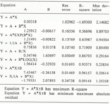
Nixon (1982) discussed the model by Konrad and Morgenstern and showed some field evidences. Using frost heave test plates at various sites, he measured the heaving rates and temperature gradient in the frozen fringe. One of the results of the measurements is summarized in Figure 4, which was drawn by the present authors using his data (Table 1, in Nixon (1982)). As both the values of the temperature gradient in the frozen fringe (grad T) and the heaving rate on various elapsed days were known, the simple regression between grad T vs. time and heaving rate vs. time were calculated. Best fits examinations were performed in each case and shown in Tables 1 and 2.

Fig. 3. Time variation of temperature profile during the freezing period in the tested soil layers.
In both cases, y = A-tB performed the best fit as the simple regression.
According to Konrad and Morgenstern, there is a simple relxtionship between grad T and V.

Fig. 4. Time variation of heave rate and temperature gradient near the frozen fringe (after Nixon 1982).
Table 1. Simple Regression Performed Between Elapsed Time (X: Days) And Temperature Gradient (Y: °C/Mm).

Equation Y = A*XtB has maximum R-square Equation Y m A*XîB has minimum maximum residual
Table 2. Simple Regressions Performed Between Elapsed Time (X: Days) And Heave Rate (Y: Mm/Day).
where SP (mm2 /s °C) is a parameter called segregation potential, which depends on soil type, and overburden pressure. If equations 3 and 4 are substituted into equation 2, then we obtain the following equation:
According to the definition, SP is constant. We assume t4x10-4 = 1 for 0 ≼ t ≼ 200 (days). Then we obtained SP value as 9 x 10⁻⁴ mm2/sec. °C. This value coincides with that estimated by Nixon (1982).
At the test site in Tomakomai, frost susceptible Tomakomai silt was used as the test soil sample. A typical result of the heaving and freezing process in winter at the site is shown in Figure 5. We had about 700 C days of freezing index at the site. Maximum heave amounts exceeded 25 cm in every winter. Temperature alternations in the layers at every 10 cm depth were recorded every 3 hours during the freezing period. The locations of 0°C isotherm and the temperature profile in the frozen fringe were estimated by the recorded data. In the early period of soil freezing, the freezing process of the soil was disturbed for a few days by warm air temperature. Thus, the temperature gradients in the frozen fringe were not stable. We observed daily freeze-thaw cycles on the surface of the ground in this period. Thus, temperature gradients in the frozen fringe (grad T) were calculated from the 1st of January. The relationship between grad T and the elapsed time from 1 January yielded grad T = A tB as the best fit among the simple regressions (Figure 6).

Fig. 5. Heave amount and frost penetration changes during freezing in the tested soil layers.

Fig. 6. The relationship between the temperature gradient near the frozen fringe and elapsed days observed at the test site. Case I.
As mentioned above, in the early period of soil freezing, heave rate alternations were not stable due to freeze-thaw cycles in the warm period. The observed heave rate alternations recorded by a displacement detector mounted on the ground surface are shown in Figure 7. Data for the calculation of simple regressions were selected from the end of December to the middle of March. Then simple regressions between heave rate and elapsed days performed v = A eB.t as the best fit.

Fig. 7. The relationship between heave rate and elapsed days at the test site. Case I.
Substituting two equations into Equation 2, SP yielded the following equation in the case of the field measurement at the site,

where SP is a parameter of Equation 2 (mm2/day-°C), t is elapsed time (day) and A, B, A’ B’ are constants. In spite of Equation 5, SP is not constant for elapsed time in Equation 6. The plot of Sp vs. time is drawn (Figure 8). According to the definition of SP, this parameter must be constant to the given soil type and the applied overburden pressure. However, in the field experiment, temperature conditions on the ground surface were not stable. These unsteady freezing conditions gave considerable effects to both the temperature and the water content profiles in the soil layers. As a result, the estimated SP parameters hold such unsteady conditions and are not constant to elapsed time.
Assuming Sp as constant, we employ two values, SP = 800 and SP = 600 (mm2/day °C). As grad T was expressed as a simple equation of time function, heaving amounts at each time might be given as follows:


Fig. 8. Time dependency of SP parameter determined by Equation 5. Case I. (Unit of SP value: mm2/day °C).

Fig. 9. Predicted and observed heave amount at the test site with two SP values. Case I.

Fig. 10. Time dependency of SP parameter in Case ?Γ. (Unit of SP value: mm2/day °C).
broken line indicates the observed heave amounts. In the case of SP = (500 (7 x 10⁻³ mm2/sec. °C), the predicted heave amount alternation conincided with the observed one.
Data from a different test site in the field were used to estimate the SP parameter ?Γ Tomakomai silt without overburden pressure (Figure 10). the equation for prediction of heave amount has a different function form from Equation 7

Substituting SP values and constants, the equation is integrated and the heaving amount curves are drawn (Figure 11). In the case of SP = 300 (mm2/day.°C), the predicted heaving amount also coincided with the observed one.
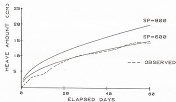
Fig. 11. Predicted and observed heave amounts at the test site with two SP values. Case II.
CONCLUSIONS
Frost heave is due to water migration toward the freezing front and accumulations in partically frozen layers forming ice-lenses. The process of water migration in soils during freezing was monitored by measurements of water content using the neutron scattering method. Water suction causes a decrease in the water content of the unforzen layers below freezing front, or 0°C isotherm, and an increase in the water content of the partially frozen layer behind the freezing front. This discontinuity of the water content profile indicates the existence of a frozen fringe, ia which ice segregations in the pores of soil take place.
The flux of water toward the frozen fringe is expressed as a simple equation (2), as proposed by Konrad and Morgenstern. The flux of water is proportional to the temperature gradients under the unsteady state condition, where the freezing front descends successively. The parameter called segregation potential (SP) is used for the prediction of heave amount based upon this concept. For the field measurements at the Tomakomai site, two SP values were estimated: one is 3.5 x 10-s mm/sec °C, and the other is 7 x 10⁻³ mm2/sec °C without overburden pressure. According to Nixon’s data, the SP value of Calgary silt was estimated as 9 x 10⁻⁴ mm2/sec °C with 100 kpa overburden pressure.
Substituting the estimated SP value into Equation 2, the field frost heaving amounts were predicted. The calculated heaving amounts coincided with the observed results. The frost heaving model based on the concept of frozen fringe was verified by the field observations.


