


INTRODUCTION
At subduction zones around the world, we see apparent mismatch between subsidence related to megathrust earthquakes and Pleistocene uplift. In a common conceptual model, interseismic strain accumulation resulting from plate locking at the subduction interface uplifts the overriding plate; a subsequent earthquake releases the strain, causing subsidence (e.g., Hyndman and Wang, Reference Hyndman and Wang1995; Clague, Reference Clague1997). Although most interseismic strain is thought to be released elastically (i.e., elastic rebound; Reid, Reference Reid1910; Whipple, Reference Whipple1936), observations indicate some strain may result in permanent deformation. For example, more than a meter of coseismic and preseismic subsidence accompanied the 2011 Tohoku-Oki megathrust earthquake (Nishimura, Reference Nishimura2014), but terraces preserved above sea level in northeast Japan record late Pleistocene uplift at rates between 0.2 and 0.46 mm/yr (Matsu'ura et al., Reference Matsu'ura, Kimura, Komatsubara, Goto, Yanagida, Ichikawa and Furusawa2015, Reference Matsu'ura, Komatsubara and Changjiang2019). In Chiloe, south-central Chile, buried soil sequences indicate coseismic subsidence (Atwater et al., Reference Atwater, Nuñez and Vita-Finzi1992; Garrett et al., Reference Garrett, Shennan, Woodroffe, Cisternas, Hocking and Gullier2015), but coastal marine terraces record Pleistocene uplift rates between 0.1 and 2 mm/yr (Melnick et al., Reference Melnick, Bookhagen, Echtler and Strecker2006; Saillard et al., Reference Saillard, Hall, Audin, Farber, Herail, Martinod, Regard, Finkel and Bondoux2009). For uplift to occur, some portion of the interseismic strain must be converted to permanent deformation. Permanent deformation may be accommodated by crustal folding or faulting or by processes related to subduction, such as sediment underplating of the overriding plate (Delph et al., Reference Delph, Thomas and Levander2021), subduction of bathymetric anomalies (e.g., Freisleben et al., Reference Freisleben, Jara-Muñoz, Melnick, Martínez and Strecker2021), mantle buoyancy (Bodmer et al., Reference Bodmer, Toomey, Roering and Karlstrom2020), or postseismic slip (e.g., Sawai et al., Reference Sawai, Satake, Kamataki, Nasu, Shishikura, Atwater, Horton, Kelsey, Nagumo and Yamaguchi2004; Kelsey et al., Reference Kelsey, Satake, Sawai, Sherrod, Shimokawa and Shishikura2006). Measurements of uplift along subduction zones on the timescale of tens to hundreds of thousands years are crucial to understanding how and why this longer-term strain accommodation departs from the elastic rebound model.
The Cascadia subduction zone (CSZ or Cascadia), located off the coast of Oregon, Washington, and northern California, USA, and British Columbia, Canada, hosts convergence between the Juan de Fuca and the North America plates (Fig. 1A). The Holocene geologic record from Washington and Oregon indicates coastal subsidence associated with Cascadia megathrust earthquakes (e.g., Atwater, Reference Atwater1987, Reference Atwater1992; Atwater and Yamaguchi, Reference Atwater and Yamaguchi1991; Witter et al., Reference Witter, Kelsey and Hemphill-Haley2003), yet, long-term coastal uplift is observed at many locations along Cascadia in the form of uplifted marine sediments and coastal topography (e.g., Palmer, Reference Palmer1967; Kelsey, Reference Kelsey1990; Kelsey et al., Reference Kelsey, Engebretson, Mitchell and Ticknor1994, 1996; Thackray, Reference Thackray1996, Reference Thackray, Stewart and Vita-Finzi1998; Padgett et al., Reference Padgett, Kelsey and Lamphear2019). Constraining the Pleistocene uplift and uplift rates along Cascadia is a first step for evaluating permanent deformation in the framework of the elastic rebound model. While other studies have documented Pleistocene coastal uplift rates in northern Washington, Oregon, and northern California, lack of detailed Quaternary mapping in southwestern Washington left a gap in our understanding.

Figure 1. Location of field area with respect to the Cascadia subduction zone (CSZ) margin. (A) The Juan de Fuca plate subducts beneath North America at about 4 cm/yr toward the northeast. Blue dashed line shows extent of the Cordilleran Ice Sheet during the last glacial maximum. Red box indicates location of B. JF, Juan de Fuca plate; NA, North America plate; OM, Olympic Mountains; QR, Quinault River; CR, Columbia River. (B) The field area is south of Grays Harbor and along Willapa Bay. Circled numbers are state highways. CHR, Chehalis River; JR, Johns River; SB, South Bend; BC, Bay Center; GP, Goose Point; PC, Pickernell Creek. Map base layer credits: Esri, Garmin, GEBCO, NOAA, NGDC, and others.
Uplifted coastal marine terraces have yielded information on deformation rates and fault activity in active tectonic settings around the world, including New Zealand (e.g., Berryman, Reference Berryman1993; Clark et al., Reference Clark, Berryman, Litchfield, Cochran and Little2010), California (e.g., Merritts and Bull, Reference Merritts and Bull1989; Lajoie et al., Reference Lajoie, Ponti, Powell, Mathieson, Sarna-Wojcicki and Morrison1991; Hanson et al., Reference Hanson, Wesling, Lettis, Kelson, Mezger, Alterman, McMullen, Cluff and Slemmons1994), and Alaska (e.g., Plafker and Rubin, Reference Plafker and Rubin1978). A marine terrace typically forms during a sea-level high stand, with the inner edge (also called the shoreline angle) of the terrace representing the former shoreline (Bradley and Griggs, Reference Bradley and Griggs1976). The inner edge serves as a horizontal datum for recording the magnitude and rate of coastal uplift (Bradley and Griggs, Reference Bradley and Griggs1976; Lajoie, Reference Lajoie and Wallace1986). Shallow crustal deformation can be measured and constrained in time if uplifted inner edges are mapped and assigned an age (e.g., Kelsey, Reference Kelsey1990; Berryman, Reference Berryman1993). Southwestern Washington is one of the few areas in Cascadia where estuarine deposits are preserved as marine terraces and therefore offers an ideal location for examining long-term sediment accumulation along an active margin for evidence of permanent deformation. The sedimentary deposits south of Grays Harbor and east of Willapa Bay (Fig. 1B) were previously mapped as a single unit (Quaternary terrace deposits, Qt) and were inferred to be Pleistocene estuarine sediments resting on marine terraces, in some locations over 160 m above sea level (asl) (Wagner, Reference Wagner1967a, Reference Wagner1967b; Kvenvolden et al., Reference Kvenvolden, Blunt and Clifton1979; Wells, Reference Wells1981; Clifton, Reference Clifton1983). This elevation for Pleistocene coastal deposits implies potentially rapid uplift rates, possibly related to regional faults (McCrory, Reference McCrory1997; McCrory et al., Reference McCrory, Foster, Danforth and Hamer2002; McCrory and Wilson, Reference McCrory and Wilson2019; Steely et al., Reference Steely, Anderson, von Dassow, Reedy, Lau, Horst and Amaral2021). The terraces offer a record of sedimentation and possible deformation that extends into the Pleistocene, but dense vegetation and limited access prevented previous workers from documenting uplift magnitude and rates.
Here, we present detailed mapping and luminescence ages to evaluate the extent and rate of Pleistocene uplift of estuarine deposits south of Grays Harbor and along Willapa Bay (Fig. 1B). Our analysis incorporates other recent luminescence dating (Steely et al., Reference Steely, Anderson, von Dassow, Reedy, Lau, Horst and Amaral2021) and previous fossil shell dating (Kennedy, Reference Kennedy1978; Kvenvolden et al., Reference Kvenvolden, Blunt and Clifton1979; Kennedy et al., Reference Kennedy, Lajoie and Wehmiller1982). The resulting uplift rate is consistent with long-term uplift rates from other studies along Cascadia. In contrast to the elastic model of earthquake cycles, we find that a small fraction of permanent uplift is permitted in the total budget for vertical land-level change, given published estimates of interseismic uplift and coseismic subsidence during subduction zone earthquakes, and this is sufficient to resolve the apparent discrepancy in short- and long-term records.
REGIONAL GEOLOGY AND TECTONICS
Washington State is situated above the Cascadia subduction zone, with the subducting margin ~100 km west of the coast (Atwater, Reference Atwater1970; Clague, Reference Clague1997; Fig. 1A). Northern Washington coastal topography is dominated by the Olympic Mountain range, an accretionary complex comprised of Eocene–Pliocene rocks that began exhumation around 16 Ma with continued active deformation to the present, shown by long-term exhumation rates for the Olympic Peninsula of ~0.3 mm/yr (Brandon and Vance, Reference Brandon and Vance1992; Brandon et al., Reference Brandon, Roden-Tice and Garver1998; Pazzaglia and Brandon, Reference Pazzaglia and Brandon2001). Along the Olympic coastline in northwestern Washington, Miocene–Pliocene nearshore and shallow-marine sedimentary units are overlain by late Pleistocene alpine glacial till and outwash. The Miocene–Pliocene nearshore and shallow-marine sedimentary units are several hundred meters above sea level (Campbell and Nesbitt, Reference Campbell and Nesbitt2000), implying uplift rates since the late Neogene of ~0.1 mm/yr or less (Pazzaglia and Brandon, Reference Pazzaglia and Brandon2001). The Quaternary sediments are broadly folded and uplifted, with uplift rates between −0.03 and 0.5 mm/yr (Thackray, Reference Thackray, Stewart and Vita-Finzi1998).
Southwestern Washington and the Willapa Hills were not glaciated in the Pleistocene, although the Olympic Mountains, north of the field area, hosted alpine glaciations throughout the Pleistocene and were a topographic high confining multiple advances of the Puget Lobe of the Cordilleran Ice Sheet to the Puget Lowlands (Booth, Reference Booth, Ruddiman and Wright1987). During the last glacial maximum, the Vashon advance, and likely during the Double Bluff advance of Marine Isotope Stage (MIS) 6, the Puget Lobe terminated south of Olympia, WA, but did not extend west around the southern side of the Olympic Mountains (Booth, Reference Booth, Ruddiman and Wright1987; Booth et al., Reference Booth, Troost, Clague and Waitt2003; Fig. 1A). Coastal southwestern Washington remained free of both continental and alpine ice throughout the Pleistocene.
Coastal topography south of the Quinault River is less pronounced than in the Olympic Mountains. Modern estuarine systems are found in Grays Harbor and Willapa Bay (Fig. 1), with highlands south of Grays Harbor and east of Willapa Bay. Regional bedrock includes basalts of the Eocene Crescent Formation (Armentrout, Reference Armentrout1987), part of the Siletzia igneous province, and associated sedimentary units that accreted to North America approximately 51 Ma (Snavely and MacLeod, Reference Snavely and MacLeod1974; Wells et al., Reference Wells, Bukry, Friedman, Pyle, Duncan, Haeussler and Wooden2014). The Crescent Formation has been folded and faulted, with folded and faulted Oligocene–Miocene sedimentary rocks in both conformable and unconformable contact with the basalts (Snavely and Wagner, Reference Snavely and Wagner1982; Armentrout, Reference Armentrout1987). Miocene basalts of the Columbia River Basalt Group are also found regionally (Armentrout, Reference Armentrout1987).
Quaternary sediment deposits at elevations up to 160 m asl are mapped onshore, proximal to the Grays Harbor and Willapa Bay estuaries. As early as 1854, Gibbs described the nearshore sediments as recording “recent” elevation change due to the presence of shell layers within the sea-cliffs (Gibbs, Reference Gibbs1854). Wagner (Reference Wagner1967a, Reference Wagner1967b) identified the sediments as undifferentiated terrace deposits (Qt) consisting of “relatively unconsolidated” clay to gravel, and with “ancient bay-fill deposits” at elevations over 100 m. Although later mapping differentiated some deposits in the southern part of Willapa Bay (Wells, Reference Wells1979, Reference Wells1981), maps continued to show the region directly south of Grays Harbor and around Willapa Bay as a single unit (Walsh et al., Reference Walsh, Korosec, Phillips, Logan and Schasse1987). The 1:250,000 scale map describes the unit as “silt, sand, and gravel of diverse composition and origins, such as … uplifted marine and estuarine deposits” (Walsh et al., Reference Walsh, Korosec, Phillips, Logan and Schasse1987).
Clifton (Reference Clifton1983) identified and described subtidal and intertidal sediment at Willapa Bay and documented that the late Pleistocene sediment exposed in sea cliffs consists of subtidal and intertidal sediment similar to what is being deposited in Willapa Bay today. These deposits were dated to the late Pleistocene based on amino acid racemization ages from bivalve shells (Kvenvolden et al., Reference Kvenvolden, Blunt and Clifton1979). Clifton (Reference Clifton1983) describes the exposed sediments as estuarine deposits of past sea-level high stands that have been uplifted since deposition. He notes that higher-elevation deposits are likely older terraces. Due to poor access, Clifton did not describe these deposits.
As part of a geotechnical study to address erosion of State Route 105, the Washington State Department of Transportation (WSDOT) used drilling and geophysical surveys to characterize shallow subsurface geology at the northwestern part of Willapa Bay, near the main tidal channel. Its work indicates dense to very dense silts and sands at depths around 20 m below sea level, underlying looser sand and Holocene sediments near sea level. WSDOT (1997) also describes a laterally extensive offshore bench (terrace) of dense sands and silts at around 9 m below sea level. They interpret these dense sediments to be the same Pleistocene terrace deposits that form cliffs along northern Willapa Bay (WSDOT, 1997), what Clifton (Reference Clifton1983) called “older terraces.”
Although regional bedrock is folded and faulted (Pease and Hoover, Reference Pease and Hoover1957; Wagner, Reference Wagner1967a, Reference Wagner1967b; Wells, Reference Wells1979, Reference Wells1981; Walsh et al., Reference Walsh, Korosec, Phillips, Logan and Schasse1987; Moothart, Reference Moothart1992), previous mapping did not indicate deformation of Quaternary deposits near Willapa Bay. Offshore studies by McCrory et al. (Reference McCrory, Foster, Danforth and Hamer2002) show faults in Willapa Bay offsetting late Pleistocene sediments, while recent mapping east of Willapa Bay shows faults that may project into the coastal Quaternary deposits (Steely et al., Reference Steely, Anderson, von Dassow, Reedy, Lau, Horst and Amaral2021).
METHODOLOGY
Geologic mapping
We revisited regions previously mapped at 1:62,000 scale as a single Quaternary terrace unit (Qt), with our mapping at approximately 1:24,000 scale (Fig. 2). Our complete geologic map, geomorphic maps, topographic profiles, stratigraphic sections, and accompanying pamphlet can be found at the University of Washington ResearchWorks archive (Stanton, Reference Stanton2021). Geomorphic analyses of slope angle and topographic smoothness on 1-m- and 10-m-resolution digital elevation models (DEMs) aided field identification of terraces (Washington State Department of Natural Resources, n.d.; U.S. Geological Survey, n.d.). We also used DEMs to identify terrace back-edge traces. Terrace mapping was supported by observations at outcrops and hand-dug pits (Fig. 3). These included hand sample and stratigraphic descriptions, gravel point counts, and where possible, depth measurements to the oxidated C-horizon (Cox horizon) in soil profiles. The Cox horizon is the location in a soil column where oxidized parent materials are encountered and represents the depth where soil-forming processes are minimal (Birkeland, Reference Birkeland1984). In the case where other soil-forming factors (relief, climate, vegetation, and parent material) are constant, time for soil development is a useful variable to discern the relative age of soils. Specifically, in the case of marine terraces on the Pacific coast, Bockheim et al. (Reference Bockheim, Kelsey and Marshall1992, Reference Bockheim, Marshall and Kelsey1996) show that depth to the Cox horizon is a useful criterion to distinguish soils of different ages. We use depth to the Cox horizon as a proxy for soil maturity and, thus, for relative age between units with similar lithologies. Twenty-three field locations provided suitable outcrop to measure the depth to the Cox horizon, with 14 of those sites within estuarine units (Qt1, Qt2, and Qss in Supplementary Table S1).

Figure 2. Geologic map of region previously mapped as Quaternary terraces. The newest mapping, done at a 1:25,000 scale, overlies geologic mapping at 1:100,000 scale (Washington Division of Geology and Earth Resources, 2016), shown here in lighter colors. Base map is 10 m digital elevation model (DEM) hill shade. See Stanton (Reference Stanton2021) for additional maps and unit descriptions. “Likely bedrock” indicates locations previously mapped as Quaternary terrace deposits that are probably bedrock. “Not accessed” indicates locations not mapped because landowners did not grant permission or because of limited road access.

Figure 3. Quaternary sediments mapped near Willapa Bay and Grays Harbor. (A) Dense, compacted silts, clays, and fine sands in unit TQss near Bruceport County Park, meter stick for scale. (B) Blue-gray silts within unit Qt2 near Bruceport County Park. Tool handle is approximately 12.5 cm long. (C) Layer of broken shells within unit Qt1 near Bay Center. Silts and fine sand layers above and below the shells. Red-handled tool from B is visible at the base of the shell layer. (D) Fine sands with silt lag deposits in unit Qss near South Bend. Secondary oxidation likely from ground water or soil processes. All photos by KMS.
Luminescence dating
Luminescence dating using feldspar grains is commonly used for deposits up to and older than 200 ka, because feldspars do not become saturated with absorbed energy at low doses, unlike quartz (Preusser et al., Reference Preusser, Degering, Fuchs, Hilgers, Kadereit, Klasen, Krbetschek, Richter and Spencer2008). Kvenvolden et al. (Reference Kvenvolden, Blunt and Clifton1979) suggest the sediments near Willapa Bay could be 120 ka or older, so we use feldspars for our luminescence dating. In our experience, quartz also tends to have low luminescence sensitivity in western Washington.
Feldspars are dated using infrared stimulated luminescence (IRSL). Although feldspar grains become saturated at much higher radioactive energy doses than quartz grains, feldspars are subject to athermal loss of the accumulated energy. This is called anomalous fading and has been explained as the leak of electrons from the traps through quantum tunneling, even when the grain has not been exposed to light. Some traps are more likely to fade than others, and the fading results in an underestimation of age. Measuring fading from laboratory-induced irradiation and extrapolating to long time periods can be used to correct for natural fading, but this works best for samples younger than 50 ka (Huntley and Lamothe, Reference Huntley and Lamothe2001).
A technique called post-infrared infrared stimulated luminescence (pIRIR; e.g., Buylaert et al., Reference Buylaert, Jain, Murray, Thomsen, Theil and Sohbati2012; Li et al., Reference Li, Jacobs, Roberts and Li2014) attempts to reduce the effect of fading by first applying a high preheat and a low-temperature IR stimulation to empty the traps more prone to fading, followed by a higher-temperature IR stimulation to tap the traps with lower fading rates (Thomsen et al., Reference Thomsen, Murray, Jain and Bøtter-Jensen2008; Jain and Ankjaergaard, Reference Jain and Ankjaergaard2011). However, these traps are also less likely to be bleached (zeroed) in nature, so pIRIR measurements can overestimate the age due to preburial partial bleaching. A new method, called post-isothermal infrared luminescence (pIt-IR; Lamothe et al., Reference Lamothe, Brisson and Hardy2020) seeks to circumvent anomalous fading without depending on hard-to-bleach traps. The technique measures low- and high-temperature IRSL after isothermal treatments that mimic natural fading until an isothermal treatment is found where the low- and high-temperature IRSL both produce the same amount of absorbed radiation, called the equivalent dose. The procedure does not eliminate fading, but rather, ensures that the density of electrons in traps is the same for both naturally irradiated and artificially irradiated feldspars, so that the true equivalent dose can be obtained (Lamothe et al., Reference Lamothe, Brisson and Hardy2020). Because the pIt-IR method avoids relying on hard-to-bleach traps, it provides a test of overestimation of age by pIRIR. If the sample is not partially bleached or contains grains of mixed ages, then the pIt-IR age should be the same as the pIRIR age. We compare dates from low-temperature IRSL with fading correction, pIRIR, and pIt-IR to see whether fading can be circumvented, as well as to detect any overestimation of age due to an unbleached residual signal from partial bleaching.
We dated eight samples to obtain sediment ages at deposits well representative of Quaternary geologic units determined from mapping (Fig. 4). Samples were collected by driving light-tight cylinders into exposed profiles. Samples collected at the mouth of the Johns River (21GW0819.5 and 20GW0713.5) were from sands within units Qt1 and Qt2, respectively (Stanton, Reference Stanton2021). Although representative of these units at these locations, their proximity to the river means these sediments may have been reworked since deposition. Samples collected near Bay Center (19GW826.1, 21GW0819.9, and 21GW0819.10) were from very fine sands within unit Qt1 (Stanton, Reference Stanton2021). In addition to dates on estuarine sediments, we also report feldspar luminescence ages from sediments collected in fluvial sands and gravels (sample 19GW827.1 in unit Qgs; Stanton, Reference Stanton2021), for sands related to the Nemah River (sample 19GW826.2 in unit Qrt; Stanton, Reference Stanton2021), and for sands and gravels near Elma, WA, mapped as undifferentiated, pre–Fraser glaciation continental glacial drift (Qgp) from the 1:250,000 regional geologic map (sample 21|GW0819.4; Walsh et al., 1987).

Figure 4. Map of luminescence sample locations with lithologic unit codes from Fig. 2 listed. Samples from this study have labels starting with 19GW, 20GW, and 21GW. Samples collected by Washington Geological Survey (Steely et al., Reference Steely, Anderson, von Dassow, Reedy, Lau, Horst and Amaral2021) are CB-OSL-561 and CB-OSL-010. Map base layer credits: Esri, Garmin, GEBCO, NOAA, NGDC, and others.
To determine the natural radiation dose rate, sample radioactivity was measured on bulk samples by alpha counting and flame photometry, as well as by beta counting. Radioactivity concentrations were translated into dose rates following Guérin et al. (Reference Guérin, Mercier and Adamiec2011). Cosmic radiation was determined after Prescott and Hutton (Reference Prescott and Hutton1988). Measured moisture contents ranged from 8 to 27%, but samples were collected in the summer (dry season), so the smaller values may underestimate typical moisture content. We used 20 ± 5% moisture content for all samples in the age calculation. Luminescence was measured on potassium feldspars, so some of the natural dose rate will arise from 40K internal to the grains. This was not measured but was estimated to be 10 ± 3%, which was recommended by Smedley et al. (Reference Smedley, Duller, Pearce and Roberts2012), although we used a slightly larger error term.
The target particles for dating were fine sand-sized single-grain (180–212 μm) potassium feldspars, because this grain size best fits the single-grain disks used for measurement. pIt-IR requires lengthy machine time, so most of those measurements were made on multi-grain aliquots, although a limited number of single-grain measurements were also made. Single-grain analysis allows an age to be computed for each grain to produce a distribution of ages for a sediment sample. An overdispersion value, a measure of spread beyond what can be accounted for by differences in precision, can be determined from this distribution of ages. The overdispersion can be accounted for by many things, such as intrinsic differences in luminescence properties among grains, differences in dose rates to individual grains, or differential fading in grains. Once these differences are accounted for, a significant spread in ages indicates mixture of ages, either because of partial bleaching of grains or postdepositional movement of grains, such as by sediment reworking by streams or tides.
We made initial low-temperature IRSL measurements at 50°C following a preheat of 250°C for 60 s. For pIRIR, we set the low-temperature stimulation at 50°C and the high-temperature stimulation at 290°C with a preheat of 320°C for 60 s. This combination has been shown to considerably reduce fading (Buylaert et al., Reference Buylaert, Jain, Murray, Thomsen, Theil and Sohbati2012). For pIt-IR measurements, we used 50 and 225°C stimulations, a 250°C, 60 s preheat, and isothermal measurements at 270°C. Single-grain measurements were made using a Risø TL/OSL DA-20 reader with an IR single-grain attachment. Stimulation used a 150 mW, 830 nm IR laser, set at 30% power and passed through an RG 780 filter. Emission was collected by the photomultiplier through a blue-filter pack, allowing transmission in the 350–450 nm range. Multi-grain single aliquots were measured on a TL.OSL DA-15 reader, using 830 nm IR diodes for stimulation. For single grains, equivalent dose (D e) was determined using the single-aliquot regenerative dose (SAR) protocol (Murray and Wintle, Reference Murray and Wintle2000), as applied to feldspars by Auclair et al. (Reference Auclair, Lamothe and Huot2003). The SAR method measures the natural signal and the signal from a series of regenerative doses on a single aliquot and uses a test dose to correct for sensitivity changes that occur during this procedure.
An advantage of single-grain dating is the opportunity to remove from analysis any grains with unsuitable characteristics by establishing a set of criteria grains must meet. Grains are eliminated from analysis if they (1) had poor signals (as judged from errors on the test dose greater than 30% or from net natural signals not at least three times above the background standard deviation); (2) did not produce, within 20%, the same signal ratio (often called recycle ratio) from identical regenerative doses given at the beginning and end of the SAR sequence, suggesting inaccurate sensitivity correction; (3) yielded natural signals that did not intersect saturating growth curves; or (4) had a signal larger than 10% of the natural signal after a zero dose and showed a visible decay.
A dose-recovery test was performed on some single grains. The luminescence was first removed by exposure to 100 s of 875 nm diodes (122 mW/cm2) and to 1 s of the laser, both at 50°C. A dose of known magnitude was then administered. The SAR procedure was then applied to see whether the known dose could be obtained. Successful recovery, shown by ratios near 1 of average derived dose to given dose, is an indication that the procedures are appropriate. The dose-recovery test also provides an overdispersion value that represents the expected overdispersion from intrinsic differences of grains in a single-age sample.
Anomalous fading (g-value) was measured using the procedures of Auclair et al. (Reference Auclair, Lamothe and Huot2003) on single grains. Ages were determined based on Aitken (Reference Aitken1985) and were corrected following Huntley and Lamothe (Reference Huntley and Lamothe2001). For pIRIR, both an uncorrected age and a fading-corrected age were obtained for each suitable grain. Even if all grains are the same true age, an identical age value is not obtained for each grain because of varying precision and other factors, including fading. Instead, as noted, a distribution is produced. The central age model (CAM) of Galbraith and Roberts (Reference Galbraith and Roberts2012) is a statistical tool used to determine the central tendency from the single-grain dates, assuming a natural distribution of estimated age values. It also computes an overdispersion parameter that can be compared to the overdispersion value of the dose-recovery test. An overdispersion value that is higher than the dose-recovery test overdispersion value may indicate partial bleaching or postdepositional mixing of grains. Similar overdispersion values from uncorrected and fading-corrected ages indicate differential fading is not causing high overdispersion.
For single-grain distributions with high overdispersion values, we employed a finite mixture model (FMM) to study the structure of the distribution. This model (Galbraith and Roberts, Reference Galbraith and Roberts2012) uses maximum likelihood to separate the grains into single-aged components based on the input of an overdispersion value thought to be typical of a single-aged sample and the assumption of a log-normal distribution for each component. We use the overdispersion values from the dose-recovery tests, which by definition are single-aged samples, to guide the selection of an appropriate overdispersion value for the FMM input. Differential within-grain K content can also increase overdispersion, but we tried to take that into account by using a higher error term on internal K than what was recommended by Smedley et al. (Reference Smedley, Duller, Pearce and Roberts2012). The FMM estimates the number of components, the weighted average of each component, and the proportion of grains assigned to each component. The FMM is most useful for samples that have discrete, rather than continuous, age populations due to mixing, although the most abundant component does not necessarily represent the most likely depositional age. Further, we assume that any mixing has occurred vertically within a stratigraphic column with similar radioactivity or between grains with a similar source. FMM can be misleading if grains from sources with a very different radioactivity are mixed. In any case, the FMM provides a structure to the age distribution, which is useful for evaluating the depositional age in a geologic context. The FMM is most usefully employed with radial graphs that visually graph the distribution of components, which we have included as Supplementary Figure S1.
RESULTS
Geology of marine deposits
Our new mapping identifies nine units within what was previously mapped only as Qt (Stanton, Reference Stanton2021; Fig. 2). Units range from shallow-marine or estuarine sands and silts, to tidal channel sands and gravels, to cross-bedded fluvial gravels and sands with occasional silt interbeds. The marine/estuarine units (units Qt1, Qt2, Qss, and TQss; Fig. 2) are found along the southern margin of Grays Harbor and along Willapa Bay (Fig. 1).
Unit TQss (late Pliocene to mid-Pleistocene shallow-marine to nearshore deposits) consists of laterally extensive, indurated, stiff, thinly bedded silts and fine sands (Fig. 3A) and massive to cross-bedded, fine to medium sands cut by oxidized, cross-bedded medium to fine sand to cobbles with silt rip-up clasts (Stanton, Reference Stanton2021). This unit forms cliffs along northern Willapa Bay. Near Bruceport, where TQss forms the sea cliffs, less indurated marine terrace sediments of unit Qt2 sit stratigraphically on top of TQss and fill embayments and channels cut into TQss. Based on geotechnical borings and seismic surveys by WSDOT (1997), we infer a bathymetric bench at approximately 9 m below sea level at northwestern Willapa Bay to be cut into unit TQss, which underlies the marine terrace deposits of unit Qt1. A wave/tide-cut bench cut into unit TQss is thus the eroded surface that younger estuarine sediments (units Qt2 and Qt1) were deposited atop.
Unit Qt2 (marine terrace deposits, MIS 5c) consists of thinly bedded, blue-gray to brown silts and fine sands and massive to cross-bedded, fine to medium sands (Fig. 3B) that form a geomorphically smooth surface between 35 and 48 m asl at numerous locations around the field area. Soils forming in unit Qt2 are orange to brown, with a depth to the Cox horizon between 1 and 2 m (Stanton, Reference Stanton2021).
We map sediments on a lower geomorphically smooth surface at between 13 and 22 m asl as unit Qt1 (marine terrace deposits, MIS 5a). Unit Qt1 consists of thinly bedded silts and fine sands with minor clay and massive to cross-bedded, fine to medium sands with silt rip-up clasts. Channel deposits, several meters to tens of meters wide, cut the finer sediments and consist of cross-bedded, medium to coarse sand to cobbles with rip-up clasts of silt and clay. The depth to the Cox horizon in soils forming in unit Qt1 is between 0.5 and 0.75 m, shallower than in unit Qt2. Based on soil maturity and elevation, unit Qt1 is presumably younger than unit Qt2. Unit Qt1 is found throughout the field area and is fossil bearing, with shell layers visible along eastern Willapa Bay within the low sea cliff (Kennedy, Reference Kennedy1978; Kvenvolden et al., Reference Kvenvolden, Blunt and Clifton1979; Stanton, Reference Stanton2021; Fig. 3C). The basal contact is not exposed, but exposures at Bay Center are up to 13 m high.
Unit Qss (silt and sand near South Bend, MIS 5e) is found only in northeastern Willapa Bay (Fig. 2) at elevations approximately 35–140 m asl. Although its total thickness cannot be estimated because basal contacts are not exposed, it is found along road cuts and within a small quarry at exposures between 6 and 8 m high. It does not form a geomorphically smooth surface, and the relationship of unit Qss to units Qt1, Qt2, and TQss is not obvious in the field. Unit Qss consists of thinly bedded, blue-gray to tan silts and clays, to bedded to massive, slightly oxidized fine sands with silt lag deposits (Fig. 3D). The silt lag deposits, or drapes, suggest a tidal environment, where tidal slack-water deposits fine grain sediments between sand ripples (e.g., Dalrymple and Choi, Reference Dalrymple and Choi2007). Depth to the Cox horizon in soils on Qss is between 1 and 1.5 m (Stanton, Reference Stanton2021). The soil maturity of Qss suggests it is older than unit Qt1, although its relative age compared with unit Qt2 cannot be determined based solely on soil maturity.
Luminescence ages
Table 1 shows concentrations of relevant radioactive elements used to calculate the total natural dose rate. Three methods for determining equivalent dose were used in this study: fading-corrected IRSL, pIRIR, and pIt-IT.
Table 1. Concentrations of elements in parts per million (ppm) or percentage (%) used to calculate natural dose and dose rate (Gy/ka).

Fading-corrected IRSL at 50°C
This procedure was only done on 19GW826.1, 19GW826.2, 19GW827.1, and 20GW0713.5. Table 2 shows the number of grains measured, the number of accepted grains, the average equivalent dose, and the average g-value (fading rate). Average fading rates range from 4 to 7%/decade. Table 3 shows the age using the CAM as well as the overdispersion value. The ratio of average derived dose to given dose in the dose-recovery test was 1.02 ± 0.3, indicating the procedure was appropriate. The overdispersion of the dose-recovery test was 13.2 ± 2.9%. The overdispersion of the samples is between 28 and 79%, much higher than the overdispersion of the dose recovery, which by design is a single-aged sample. This suggests the samples could be of mixed age.
Table 2. Grains measured, the number accepted for dating, the average equivalent dose (Gy) from the central age model (CAM) and the average g-value (fading rate).

a IRSL, infrared stimulated luminescence.
b pIRIR, post-infrared infrared stimulated luminescence.
c A decade is a power of 10. By convention, the g-value is standardized to a time constant of 2 days, so that successive decades are 2, 20, 200, 2000 days, etc.
d Long dash (—) indicates no data were collected.
e A weighted average for this value is 2.3 ± 1.1%.
f A weighted average for this value is 0.02 ± 3.9%.
Table 3. Ages and overdispersion values for infrared stimulated luminescence (IRSL) at 50°C and for post-infrared infrared stimulated luminescence (pIRIR) at 290°C using the central age model (CAM).a

a Ages are either corrected for anomalous faded or uncorrected, and are quoted with 1-sigma errors, using 2021 as the reference for before present designations.
b Long dash (—) indicates no data were collected.
Post-IRIR at 290°C
Table 2 shows the grains measured and accepted, as well as the average equivalent dose and the average fading rate. Average fading rates range between 0.6 and 6%/decade. No fading test was conducted on 20GW0713.5. Only two samples, 19GW826.1 and 21GW0819.5, show fading rates significantly above 1.5%/decade, but weighted averages for those two samples are not significantly above that value. Buylaert et al. (Reference Buylaert, Jain, Murray, Thomsen, Theil and Sohbati2012) consider fading rates that low to be artifacts of measurement. Table 3 gives the age using the CAM as well as the overdispersion value for the pIRIR at 290°C signal, using both fading-corrected and uncorrected data. The overdispersion values for corrected data and uncorrected data are similar, suggesting that the fading correction did not reduce the age scatter. Similarity in ages between corrected and uncorrected data also show that fading in the pIRIR signal is likely not significant, and only the uncorrected ages are considered further. Radial graphs (Supplementary Fig. S1), explained in the caption, show the distribution of single-age grains for the uncorrected ages from pIRIR at 290°C measurements. A dose-recovery test was performed on 100 grains from 19GW826.1. The ratio of average derived dose to administered dose was 1.10 ± 0.05, which is satisfactory at 2-sigma, but not as good as the dose recovery in the IRSL dose-recovery test. The overestimation for the pIRIR at 290°C dose-recovery test may reflect the greater difficulty in bleaching for that signal, which may not have been completely zeroed before the dose was administered. Overdispersion for the pIRIR at 290°C dose-recovery test was 14.4 ± 4.3%, nearly the same as for the IRSL dose-recovery test. As with the IRSL, the high overdispersion values of the samples (Table 3) compared with the dose-recovery test overdispersion value suggests the samples could be of mixed ages, so the age distributions for the pIRIR at 290°C were evaluated using an FMM. The FMM divides the distribution into single-aged components assuming a normal distribution and inputting overdispersion values thought to be typical of a single-aged sample. The overdispersion used was 15%, just slightly higher than what was obtained from the dose-recovery test. Table 4 shows the results from the FMM. Sample 19GW826.1 resolved in a single component for the corrected data, and 76% of the grains were consistent with one component in the uncorrected data. About 70–75% of the grains were consistent with one component for both corrected and uncorrected data for 19GW826.2. All other samples resolved into multiple component mixtures.
Table 4. Finite mixture model ages for post-infrared infrared stimulated luminescence (pIRIR) at 290°C.a

a Ages are either corrected or uncorrected for anomalous fading, and are quoted with 1-sigma errors, using 2021 as the reference for before present designations.
pIt-IR
The pIt-IR procedure was run on multi-grain aliquots for samples 19GW826.1, 20GW0713.5, 21GW0819.4, 21GW0819.5, and 21GW0819.9. The procedure was done on two to three aliquots for each sample. A limited number of single-grain pIt-IR measurements were made on 19GW826.2 and 19GW827.1, but the analysis showed that only a handful of grains from each sample were acceptable. This was not enough to do a distributional analysis of their ages, so the single-grain pIt-IR analysis was abandoned. No pIt-IR measurements were done on 21GW0819.10 because of limited material.
The pIt-IR ages are given in Table 5 along with the uncorrected pIRIR at 225°C ages, which were done in conjunction with pIt-IR. In samples 21GW0819.4 and 21GW0819.9, the pIt-IR age is much older than the pIRIR at 225°C age. This may be an indication that the samples were not well bleached before burial. It is believed that pIt-IR will badly overestimate the age if the sample is poorly bleached (Lamothe et al., Reference Lamothe, Brisson and Hardy2020), although the exact effect of poor bleaching is still under study. For samples 19GW826.1, 20GW0713.5, and 21GW0819.5, there is agreement between the pIt-IR age and the pIRIR at 225°C age. This indicates that these samples are well bleached.
Table 5. Ages averaged from two or three multi-grain aliquots for post-isothermal infrared luminescence (pIt-IR) and for post-infrared infrared stimulated luminescence (pIRIR) at 225°C collected in conjunction with pIt-IR.a

a Ages are quoted with 1-sigma errors, using 2021 as the reference for before present designations.
b pIRIR at 225°C ages are not corrected for anomalous fading.
DISCUSSION
Age
In the Willapa Bay and Grays Harbor region, estuarine units (Qt1 and Qt2) are deposited on benches cut into the older unit TQss. Wave-cut or tide-cut benches and the associated back edges are assumed to form during sea-level high stands (Bradley and Griggs, Reference Bradley and Griggs1976; Lajoie, Reference Lajoie and Wallace1986), which during the Quaternary correlate to odd-numbered MIS determined from benthic δ18O records (Lisiecki and Raymo, Reference Lisiecki and Raymo2005). Even-numbered MIS are sea-level low stands associated with continental ice-sheet advances. We discuss relative soil maturity, luminescence ages, and previous dating based on fossil shells to determine the most likely MIS (and thus depositional age) for each estuarine unit (Qt1, Qt2, and Qss).
Soil development with elevation
Silts and sands make up the estuarine units (Qt1, Qt2, and Qss). Numerous studies use the depth to the Cox horizon as proxy for soil maturity and, thus, to assess the relative age between similar sediments experiencing the same climatic conditions (e.g., Birkeland, Reference Birkeland1984; Kelsey, Reference Kelsey1990; Padgett et al., Reference Padgett, Kelsey and Lamphear2019). For this study, the depth to the Cox horizon in unit Qt1 (n = 3), the lowest-elevation deposit, ranges between 0.5 and 0.75 m, with the depth to the Cox horizon in unit Qt2 (n = 6), the next highest elevation deposit, ranging between 1 and 2 m, and in unit Qss, the highest-elevation deposit, between 1 and 1.5 m (n = 5). The relative age of units Qt2 and Qss cannot be determined from soil development alone, but both are likely older than unit Qt1.
Luminescence
In our single-grain analyses for both fading-corrected IRSL and pIRIR, most of the samples show a large overdispersion of ages when compared with a dose-recovery test, suggesting that mixing may have occurred, either by partial bleaching of grains before deposition or by postdepositional movement of grains. We evaluate the ages of the samples using the results of the CAM and FMM for pIRIR and using the ages from the IRSL and pIt-IR techniques. The fading rates (g-values) are relatively small, and we do not have fading-corrected data for all samples. We use the ages from uncorrected data in our discussion. Table 6 presents the most likely ages for pIRIR at 290°C for all samples. We focus on the estuarine samples (19GW826.1, 20GW0713.5, 21GW0819.5, 21GW0819.9, 21GW0819.10) here. The non-estuarine samples are from fluvial and glacial units and not pertinent to the Pleistocene uplift in the field area, although dating the samples contributed to the new Quaternary map (Stanton, Reference Stanton2021). For a discussion of the ages of the non-estuarine samples (19GW827.1, 19GW826.2, 21GW0819.4), please see the Supplementary Text. We also include in Table 6 dates from optically stimulated luminescence (OSL; using quartz) samples (CB-OSL-561, CB-OSL-101) collected by the Washington Geological Survey (WGS) and dated at Utah State University (Steely et al., Reference Steely, Anderson, von Dassow, Reedy, Lau, Horst and Amaral2021) from sites that we have correlated to our newly mapped estuarine units.
Table 6. Summary of luminescence ages.a

a Post-infrared infrared stimulated luminescence (pIRIR) ages quoted with 1-sigma errors, using 2021 as the reference for before present designations. Single-grain ages evaluated using a finite mixture model (FMM; Galbraith and Roberts, Reference Galbraith and Roberts2012). Mixture model component ages (e.g., FMM 2nd) provide constraint on the most likely depositional ages as assessed by the likelihood of partial bleaching and sediment reworking, listing two where there were bimodal age distributions. Ages are uncorrected for fading. Long dash (—) indicates no data were collected. CAM, central age model; OSL, optically stimulated luminescence.
b All samples with labels starting with 19GW, 20GW, and 21GW were dated using pIRIR at 290°. Washington Geological Surveys samples (samples CB-OSL-561 and CB-OSL-010) were dated using OSL at Utah State University. See Steely et al. (Reference Steely, Anderson, von Dassow, Reedy, Lau, Horst and Amaral2021) for details.
c Sample collected outside field area from sand and gravels near Elma, WA, mapped as Qgp, undifferentiated pre–Fraser glaciation continental glacial drift from 1:250,000 regional geologic map (Walsh et al., Reference Walsh, Korosec, Phillips, Logan and Schasse1987).
Samples 19GW826.1 and 21GW0819.10 are from the same stratigraphic section just above the beach at Bay Center in unit Qt1 marine terrace sediments. Sample 19GW826.1 is above and sample 21GW0819.10 is below a layer of shells. The FMM (Table 4) suggests that 19GW826.1 conforms to a single-aged sample with no evidence of partial bleaching or postdepositional movement. The agreement in age between pIRIR and pIt-IR supports this. The CAM (Table 3) should therefore give a good estimate of the age. The uncorrected value is 74.8 ± 3.21 ka, in good agreement with the pIt-IR age (Table 5). This agreement also suggests that the pIRIR signal is well bleached. The fading-corrected age of the 50°C IRSL measurement is substantially lower than all other ages, suggesting that the Huntley-Lamothe fading correction is not effective for this aged sample. We do not consider the fading-corrected IRSL measurements for further samples. The CAM date for 19GW826.1 anchors our interpretation of FMM results for other samples.
Sample 21GW0819.10 suffers from small sample size because of limited material available. It also seemed to have been contaminated with younger grains. The FMM (Table 4) suggests a large portion of grains, about a third, is in the 18–14 ka range. This does not agree with the data from sample 19GW826.1 and could represent contamination, possibly during sampling. The second FMM component in the uncorrected data suggests that the age could be 70.2 ± 7.35 ka if the sample was poorly bleached before burial so that the second component represents the true youngest grains. This age is within error range of sample 19GW826.1 and would represent rapid deposition. Given the high overdispersion values, partial bleaching is probably the best interpretation, making the ~70 ka age the best estimate and explaining the presence of older grains (third FMM component).
Sample 21GW0819.9 is from the east side of Willapa Bay, also from a section mapped as unit Qt1 marine terrace sediments. The pIt-IR analysis (Table 5) suggests partial bleaching, giving a likely overestimated age of 188 ± 23 ka compared with the pIRIR analyses (at 225°C and 290°C). The youngest component of the FMM (Table 4) suggests a small portion of very young grains, probably contamination. The second component gives an age of 74.5 ± 7.61 ka. This is consistent with the ages from samples 19GW826.1 and 21GW0819.10. There are older grains within the sample, which supports the partial bleaching interpretation.
We correlated our luminescence ages to MIS (Lisiecki and Raymo, Reference Lisiecki and Raymo2005) for the mapped estuarine units near Willapa Bay (Table 7). Within error, each luminescence sample date could correspond to one of several different MIS. For example, samples 19GW826.1, 21GW0819.10, and 21GW0819.9 could have formed during MIS 4 or MIS 5a. MIS 4 was a sea-level low stand, and estuarine sediments were unlikely to have been deposited in Willapa Bay at that time, leaving the MIS 5a age as the most likely.
Table 7. Age determinations for uplifted estuarine units correlated to marine isotope stages (MIS), with ages quoted with 1-sigma errors, using 2021 as the reference for before present designations.a

a Long dash (—) indicates no data were collected. OSL, optically stimulated luminescence; pIRIR, post-infrared infrared stimulated luminescence.
b Within error, some samples correlate to several MIS.
c See Steely et al. (Reference Steely, Anderson, von Dassow, Reedy, Lau, Horst and Amaral2021) for details.
The ages are not as straightforward for sample 20GW0713.5 in unit Qt2 and sample 21GW0819.5 in unit Qt1, both obtained from the mouth of the Johns River where it empties into Grays Harbor. The very large overdispersion values suggest mixing. The youngest FMM component (Table 4) of sample 21GW0819.5 (component 1 of uncorrected data) represents a small percentage of grains at a very young age and likely represents contamination. Disregarding this contaminated age, the ages from the youngest FMM components in uncorrected data are 49.1 ± 10.8 ka for 20GW0713.5 and 20.8 ± 1.63 ka for 21GW0819.5. The oldest FMM components in uncorrected data give ages of 162.4 ± 13.4 ka for 20GW0713.5 and 129 ± 11.4 ka for 21GW0819.5. These mixtures could result from older sediments being partially reset sometime after deposition to give some younger-aged grains. In this case, the deposit sampled would be the older age, with later, partial reworking or bleaching of sediments. Alternatively, the samples could be from sediment deposited more recently, but with most grains retaining a residual charge resulting from incomplete bleaching before burial. The pIt-IR ages (Table 5) are 162 ± 13.4 ka for 20GW0713.5 and 124 ± 15.6 ka for 21GW0819.5, in agreement with the oldest FMM components in the pIRIR uncorrected data. The agreement between pIt-IR and pIRIR ages might suggest the samples were not partially bleached at all, but if that is the case, then the origin of the younger component needs explaining. It is also possible that the river has continually reworked the sediments. In that case, perhaps none of the luminescence ages for these samples represents the depositional age of the sediments forming unit Qt2 and unit Qt1 at this location. Additional dating of the terraces at the Johns River would be required to say something more concrete about the depositional ages and processes at work.
We use the ages of the OSL samples collected by the WGS (Steely et al., Reference Steely, Anderson, von Dassow, Reedy, Lau, Horst and Amaral2021) in our age interpretation of Quaternary units (Table 6). Based on the sample location, sample CB-OSL-561 (95.42 ± 15.02 ka) is from silts and fine sands within an embayment near Bruceport (Fig. 4). We interpret the sediments to be part of unit Qt2, deposited within a drainage or embayment cut into unit TQss. The WGS location for sample CB-OSL-101 (119.64 ± 23.91 ka) places it within sands in a small sand quarry near South Bend (Fig. 4) that we correlate to unit Qss. The OSL dates provide a depositional age of MIS 5a, 5c, or 5d for unit Qt2 and a depositional age of MIS 5c, 5e, or 6 for unit Qss (Table 7). Despite the larger error compared with our IRSL dates, the OSL dates suggest that units Qt2 and Qss at eastern Willapa Bay are likely older than the MIS 5a unit Qt1.
Taken together, luminescence ages from all samples suggest an increasing age for sediments found at increasing elevations. With the exception of dates for the samples near the Johns River that may indicate reworking, the ages of progressively higher estuarine deposits are also sequential, as would be expected from estuarine sediments deposited during different sea-level high stands that have been uplifted through time.
Fossil shells
Kvenvolden et al. (Reference Kvenvolden, Blunt and Clifton1979) used amino acid racemization to date fossil shell fragments from low cliffs near Bay Center in eastern Willapa Bay (unit Qt1). They obtained a mean d/l leucine ratio of 0.31 (n = 48) and a calculated date of 120 ± 40 ka. They admit that their date is highly dependent on both the actual temperature of Willapa Bay through time and the actual age of the calibration location in California.
Kennedy (Reference Kennedy1978) and Kennedy et al. (Reference Kennedy, Lajoie and Wehmiller1982), using a combination of dating methods, provided probable ages for Pleistocene fauna along the West Coast from Washington to central California. They note that southern extralimital species (i.e., warm water) are found on independently dated MIS 5e terraces, while northern extralimital species (i.e., cool water) are found on independently dated MIS 5c and 5a terraces. They then correlate species type and amino acid racemization d/l leucine ratios from poorly dated locations to those from independently dated terraces. Amino acid racemization d/l leucine ratios on two whole bivalve shells from the low cliffs at Bay Center (unit Qt1) are 0.29 and 0.317, which they correlate to MIS 5a (or about 84 ka).
The age obtained by Kvenvolden et al. (Reference Kvenvolden, Blunt and Clifton1979) corresponds to MIS 5e but overlaps within error to an MIS 5a age. Kennedy (Reference Kennedy1978) and Kennedy et al. (Reference Kennedy, Lajoie and Wehmiller1982) reject an MIS 5e age for these shells, because the d/l leucine ratios from both their study as well as from Kvenvolden et al. (Reference Kvenvolden, Blunt and Clifton1979) are much lower than at other coastal locations that are independently dated to MIS 5e. The presence of a supposed cool-water species in the lower terrace deposits at Willapa Bay supports assignment of this deposit to MIS 5a (Kennedy et al., Reference Kennedy, Lajoie and Wehmiller1982), although Kennedy (Reference Kennedy1978) admits that more southerly conditions (i.e., warm water) is a possibility.
In addition to dating shells in the low cliffs near Bay Center, Kennedy (Reference Kennedy1978) also used amino acid racemization dating on shells collected at cliff exposures along northern Willapa Bay (our unit TQss). Addicott (Reference Addicott1974) provides a late Pliocene to Early Pleistocene age for these deposits based on the correlation of a fossil shallow-marine or estuarine mollusk (Mytilus condoni Dall) to dated deposits in northern California. More recent work on the northern California deposits suggests they may be as young as mid-Pleistocene (Meyer et al., Reference Meyer, Sarna-Wojcicki, Hillhouse, Woodward, Slate and Sorg1991). Kennedy (Reference Kennedy1978) obtains d/l leucine ratios of 0.81, corresponding to an age of around 1.5–1.3 Ma based on age correlations elsewhere along the coast. Kennedy (Reference Kennedy1978) does note that this age is far from exact, but it supports an Early Pleistocene age for unit TQss.
Age summary
Based on soil maturity, units Qt2 and Qss are both older than unit Qt1. Based solely on elevation, Qss is likely also older than unit Qt2, because it is found at a consistently higher elevation than Qt2, thus implying that the sediments have been uplifted for a longer period of time. Fossil shells found in unit Qt1 provide an age either of MIS 5a (Kennedy, Reference Kennedy1978) or MIS 5e (Kvenvolden et al., Reference Kvenvolden, Blunt and Clifton1979). Assuming these preserved marine terrace sediments were deposited during sea-level high stands only, IRSL dating provides an age of 5a for Qt1. OSL dating provides an age of either MIS 5a or 5c for Qt2, and of either MIS 5c or 5e for Qss. Both the luminescence ages and the soil maturity suggest an age progression of youngest sediments at low elevation to oldest sediments at high elevation.
The date for fossil shells in unit Qt1 provided by Kvenvolden et al. (Reference Kvenvolden, Blunt and Clifton1979) has a large error of 40 ka. Within error, their date could be as old as 160 ka (MIS 6) or as young as 80 ka (MIS 5a). If their date of 120 ka (MIS 5e) is correct, then all luminescence ages for all samples are incorrect, because all sediments at higher elevations, with increased soil maturity, must be older than MIS 5e. If, however, their younger date within error is correct (MIS 5a), it correlates to the age determined for unit Qt1 from fossil shells by Kennedy (Reference Kennedy1978) as well with our IRSL dates.
In summary, our age assignments for the late Pleistocene estuarine units are MIS 5a for unit Qt1, MIS 5c for unit Qt2, and MIS 5e for unit Qss. Based on crosscutting relationships and superposition, unit TQss is older, and thus likely Pliocene to mid-Pleistocene, as suggested by fossil shells.
Uplift and uplift rates
The sediments (units Qt1 and Qt2) underlying the geomorphically smooth surfaces we have called terraces are estuarine in nature and are therefore deposited in proximity to sea level. Uplift of estuarine or marine deposits is the difference between the modern elevation and the sea-level elevation (compared with modern) at the time of sediment deposition. Uplift calculations for marine terraces typically use the elevation of the inner edge of the terrace, because a terrace inner edge represents the location of the former sea cliff and therefore can be used as a datum approximating mean high water (Bradley and Griggs, Reference Bradley and Griggs1976; Lajoie, Reference Lajoie and Wallace1986; Keller and Pinter, Reference Keller and Pinter2002; Fig. 5). We estimate the inner-edge elevation by subtracting the range of minimum cover-sediment thickness from the terrace back-edge elevation.
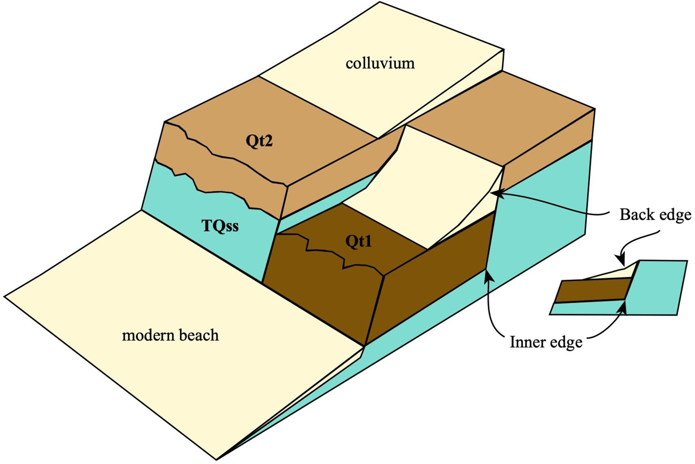
Figure 5. Block diagram illustrating the relationship of estuarine units Qt1 and Qt2 to unit TQss. Unit Qss is also estuarine, but the relationship to other estuarine units could not be determined in the field, and it is not included in this diagram. Also shown are the locations of the back edge and the inner edge of the terrace. The back-edge elevation is determined by the average elevation of remnant back-edge fragments from 1 m digital elevation models (DEMs). The inner-edge elevation is estimated by subtracting the estimated sediment thickness from the back-edge elevation.
We identify the back edge as the position of greatest change in surface slope in the region between two terraces (Fig. 5). In the study area, the terraces have a range of elevations (13–22 m for the lower terrace and 35–48 m for the upper terrace) and are eroded and dissected by streams. Distinct back edges are generally obscured, except as fragments, which we traced on LIDAR and the 10 m DEM for both lower and upper terraces. We used standard GIS tools to determine the elevation and elevation standard deviation of these traces. This provides a mean back-edge elevation for the lower terrace (overlain by unit Qt1) of 21 ± 3 m and of 42 ± 8 m for the back edge of the upper terrace (overlain by unit Qt2).
The estuarine sediment units Qt1 and Qt2 overlie wave-cut or tide-cut strath surfaces eroded into older sediments. Unit Qt2 (marine terrace deposits, MIS 5c) consists of sediments that sit on top of the Early Pleistocene TQss unit. Qt2 also fills embayments and drainages cut into TQss. This implies that the younger Qt2 was deposited on an eroded surface of TQss. Where visible in the modern sea cliff, Qt2 is approximately 2–4 m thick above TQss, but exposures of this contact are limited to the northern part of Willapa Bay, and it is possible that these exposures of the contact between TQss and Qt2 are not representative of the region. For comparison, the exposures of unit Qt1 (marine terrace deposits, MIS 5a) near Bay Center are 8–13 m thick, with no exposures of the wave-cut TQss underlying Qt1. Work by WSDOT identifies the older terrace unit (TQss) as forming a bench at ~9 m below sea level at northwestern Willapa Bay with up to 9 m of dense sand and silt (perhaps Qt1) and several meters of Holocene beach sand above it (WSDOT, 1997). Additionally, exposures of Qt2 near the Johns River in southern Grays Harbor show 6–9 m of sands and silts without exposing a contact with TQss. These exposures may include material deposited from the Johns River, however. We estimate that eroded surfaces in TQss are 9 ± 5 m below the upper surfaces of the terraces, at a minimum. This thickness of sediments for units Qt1 and Qt2 is consistent with sediment thicknesses overlying marine terraces at other places in Cascadia (e.g., Kelsey, Reference Kelsey1990; McInelly and Kelsey, Reference McInelly and Kelsey1990; Polenz and Kelsey, Reference Polenz and Kelsey1999; Kelsey and Bockheim, Reference Kelsey and Bockheim1994; Padgett et al., Reference Padgett, Kelsey and Lamphear2019), although those locations are more exposed to wave processes than the estuarine environment of northern Willapa Bay.
The inner edge (also called the “shoreline angle”) represents sea level as eroded by breaking waves (Bradley and Griggs, Reference Bradley and Griggs1976; Lajoie, Reference Lajoie and Wallace1986; Keller and Pinter, Reference Keller and Pinter2002). In an estuary, erosion may occur from both waves and tidal current. Willapa Bay, a macrotidal estuary, has a tidal range between 1.25 and 3 m (Emmett et al., Reference Emmett, Llanso, Newton, Thom, Hornberger, Morgan, Levings, Copping and Fishman2000; Banas and Hickey, Reference Banas and Hickey2005), and we use the modern mean tidal range for Willapa Bay of ±2 m (6.8 ft; Michalsen et al., Reference Michalsen, Babcock and Lin2010) as a minimum error for inner-edge elevation based on tidal fluctuation. Therefore, the uncertainty in the assigned elevation of the inner edge (e. g., shoreline angle) is ±2 m.
Paleo–sea level high-stand elevations have typically been reported as global mean, or eustatic, sea levels estimated from dated sea-level markers in regions of limited tectonic activity. These can vary widely. For example, studies from Bermuda and the Bahamas estimate MIS 5a eustatic sea level at approximately the same as modern sea level (Vacher and Hearty, Reference Vacher and Hearty1989; Hearty and Kindler, Reference Hearty and Kindler1995), while other estimates place MIS 5a eustatic sea level at ~ −19 ± 5 m (Chappell and Shackleton, Reference Chappell and Shackleton1986). More recently, recognition of the importance of glacial isostatic adjustment (GIA) has led to the development of geodynamic models whereby relative sea level locally can vary from global mean sea level as a response to expansion and contraction of ice sheets (Creveling et al., Reference Creveling, Mitrovica, Hay, Austermann and Kopp2015, 2017; Simms et al., Reference Simms, Rouby and Lambeck2015). Along the West Coast of North America, relative sea level may have varied regionally up to 30 m during MIS 5c and up to 35 m during MIS 5a (Creveling et al., Reference Creveling, Mitrovica, Clark, Waelbroeck and Pico2017). Additionally, relative sea level at a single site may vary over the interval of a particular MIS. Although estimates of an MIS sea-level high stand based on site-specific GIA would provide the most accurate estimate of total uplift, detailed modeling for most of Cascadia is currently unavailable. Similar to other recent uplift studies in Cascadia (e.g., Padgett et al., Reference Padgett, Kelsey and Lamphear2019), our study uses the range of mean sea level for MIS 5a and 5c based on geodynamic modeling at a location close to the field area, in this case, from Coquille, OR (Creveling et al., Reference Creveling, Mitrovica, Clark, Waelbroeck and Pico2017); thus, mean paleo–sea level is −19 ± 7 m for MIS 5a and −10 ± 7 m for MIS 5c.
Given these inputs, we estimate the total uplift for the inner edge of the terraces as:

where PSL is the paleo–sea level and MSL is mean sea level, taken here to be the mean tidal range. To obtain an uncertainty in uplift, we propagate the uncertainty for the variables using addition in quadrature (also called the square root of the sum of the squares; Taylor, Reference Taylor1997). Given these inputs and assigning an MIS 5a age to Qt1 and an MIS 5c age to Qt2, the total uplift for the Qt1 terrace is 31 ± 9 m, and the total uplift for the Qt2 terrace is 43 ± 12 m (Table 8).
Table 8. Uplift rates for terraced estuarine sediments near South Bend, WA.

a Terrace back-edge elevation estimated from eroded traces on digital elevation model (DEM).
b Minimum sediment thickness from Qt2 exposures at modern sea cliffs near Bay Center. Qt1 sediment thickness is at least 14 m, greater than the lowest terrace surface elevation of ~13 m. Sediment thickness is thus 9 ± 5 m.
c Wave-cut benches mark mean sea level, which varies with tides and storms. We use the tidal fluctuation for Willapa Bay of ±2 m (Michalsen et al., 2010).
d Paleo–sea level elevation has not been modeled for the field area, so we used the range of elevations at Coquille, OR, from geodynamic models (Creveling et al., Reference Creveling, Mitrovica, Clark, Waelbroeck and Pico2017).
e Uplift is the difference between the paleo–sea level elevation and the current elevation of the inner edge (back edge minus sediment thickness) ± the sea-level fluctuation.
f Marine Isotope Stage (MIS) peak age, with an uncertainty of ±4 ka (Lisiecki and Raymo, Reference Lisiecki and Raymo2005).
g Uplift rate is the total uplift divided by the age of the terrace surface. Uncertainty calculated using standard error propagation methods.
Unit Qss consists of estuarine sands and silt but does not form a geomorphically smooth surface with a distinct back edge. We do not have evidence of a wave/tide-cut surface that Qss sediments sit on, nor do we have an estimate of the sediment thickness. We thus cannot assess the total uplift of unit Qss.
We calculate the late Pleistocene uplift rates for units Qt1 and Qt2 terraces as

where age is the time since deposition (Table 8). Again, we propagate the uncertainty of these values to obtain uncertainty to the uplift rate (see Supplementary Table S2 for ranges of uplift rates). We are using uplift of the inner edge of the terraces for units Qt1 and Qt2, which presumably formed during peak sea-level high stands, so we use the peak ages for the sea-level high stands based on recent studies of global benthic δ18O records, which have an uncertainty of ±4 ka (Lisiecki and Raymo, Reference Lisiecki and Raymo2005). The preferred ages are 82 ± 4 ka (MIS 5a) for unit Qt1 terrace and 96 ± 4 ka for Qt2 terrace (MIS 5c). Given these ages, the maximum uplift rates are 0.4 ± 0.12 mm/yr for Qt1 and 0.4 ± 0.13 mm/yr for Qt2 (Table 8).
There is significant uncertainty in paleo–sea level elevation, as noted previously, with eustatic estimates and geodynamic models providing different values. For terraces underlying units Qt1 and Qt2, uplift rates are calculated using GIA-adjusted paleo–sea level high-stand elevations from Coquille, OR. For comparison, we calculate uplift rates for the terraces using estimates of global eustatic paleo–sea level elevation (Supplementary Table S3) as well as estimates of GIA-adjusted paleo–sea level elevation near to the field area from Simms et al. (2015; Supplementary Table S4). The uplift rates using global eustatic sea level are 0.1–0.5 mm/yr for unit Qt1 terrace and 0.3–0.5 mm/yr for unit Qt2 terrace, while the uplift rates using sea level from Simms et al. (Reference Simms, Rouby and Lambeck2015) are 0.2–0.6 mm/yr for unit Qt1 terrace and 0.4–0.7 mm/yr for unit Qt2 terrace. The uplift rates using paleo–sea level elevations for Coquille, OR (Creveling et al., Reference Creveling, Mitrovica, Clark, Waelbroeck and Pico2017) are within the range of uplift rate estimates that do not employ GIA-adjusted, paleo–sea level high-stand estimates.
Comparison with other Cascadia Pleistocene uplift rates
Pleistocene uplift rates in Cascadia based on uplifted marine terraces, as well as long-term stream incision rates averaged over >10 ka, range between −0.03 and 1.8 mm/yr, comparable to rates for coastal southwestern Washington from this study (Fig. 6). Deformation of a folded wave-cut surface and glacial outwash sediments at Kalaloch, WA, just north of Grays Harbor, includes uplift rates between −0.03 and 0.5 mm/yr, depending on the age of the wave-cut surface (Thackray, Reference Thackray, Stewart and Vita-Finzi1998; Fig. 6, site 1). If formed during MIS 7, the vertical deformation consists of uplift only. If formed during MIS 5e, vertical deformation may include minor subsidence (Thackray, Reference Thackray, Stewart and Vita-Finzi1998). The Clearwater River in the western Olympic Mountains shows long-term incision rates between 0.1 and 0.9 mm/yr, although the uplift inferred from the incision rates is interpreted as related to growth of the Olympics only, with Pazzaglia and Brandon (Reference Pazzaglia and Brandon2001) noting that Pliocene marine sediments on the coast have elevations near to their formation elevation based on distribution of foraminifera (Pazzaglia and Brandon, Reference Pazzaglia and Brandon2001; Pazzaglia et al., Reference Pazzaglia, Thackray, Brandon, Wegmann, Gosse, McDonald, Garcia, Prothero and Swanson2003; Fig. 6, site 2). Stream incision on the Wynoochee River (north and east of our study area) shows incision rates as high as 1.8 mm/yr associated with a local fault (Delano et al., Reference Delano, Amos, Loveless, Rittenour, Sherrod and Lynch2017; Fig. 6, site 3). Incision of coastal Oregon streams shows rates up to 1.3 mm/yr (Personius, Reference Personius1995; Fig. 6, sites 5–13). Late Pleistocene marine terraces in Oregon show uplift rates between 0 and 1.4 mm/yr, with higher rates associated with folding or faulting (Kelsey, Reference Kelsey1990; Muhs et al., Reference Muhs, Kelsey, Miller, Kennedy, Whelan and McInelly1990, Reference Muhs, Rockwell and Kennedy1992; McInelly and Kelsey, Reference McInelly and Kelsey1990; Ticknor, Reference Ticknor1993; Kelsey et al., Reference Kelsey, Engebretson, Mitchell and Ticknor1994, 1996; Kelsey and Bockheim, Reference Kelsey and Bockheim1994; Fig. 6, sites 14–20). Marine terraces in northern California show uplift rates between 0 and 1.05 mm/yr, associated with regional folding (Polenz and Kelsey, Reference Polenz and Kelsey1999; Padgett et al., Reference Padgett, Kelsey and Lamphear2019; Fig. 6, sites 21, 22). In all studies, uplift rates of ~0.5 mm/yr and greater are associated with local folds or faults (see Supplementary Tables S5–S7 for additional details on rates and studies).

Figure 6. (A) Uplift and incision rates along the Cascadia margin. (B) Uplift and incision study sites. Circles are uplifted marine terraces. Triangles are incision rates. Orange indicates known local structures may affect uplift rate. Blue indicates local structures have not been identified. Rates discussed in more detail in the text. Supplementary Tables S5–S7 provide additional details on studies and uplift rates. Sources: (1) Thackray, Reference Thackray1996, Reference Thackray, Stewart and Vita-Finzi1998; (2) Pazzaglia and Brandon, Reference Pazzaglia and Brandon2001; (3) Delano et al., Reference Delano, Amos, Loveless, Rittenour, Sherrod and Lynch2017; (5–13) Personius, Reference Personius1995; (14–16) Kelsey et al., Reference Kelsey, Ticknor, Bockheim and Mitchell1996; Ticknor, Reference Ticknor1993; (17) McInelly and Kelsey, Reference McInelly and Kelsey1990; Muhs et al., Reference Muhs, Kelsey, Miller, Kennedy, Whelan and McInelly1990, Reference Muhs, Rockwell and Kennedy1992; Kelsey et al., Reference Kelsey, Engebretson, Mitchell and Ticknor1994; (18) Kelsey, Reference Kelsey1990; Muhs et al., Reference Muhs, Kelsey, Miller, Kennedy, Whelan and McInelly1990, Reference Muhs, Rockwell and Kennedy1992; Kelsey et al., Reference Kelsey, Engebretson, Mitchell and Ticknor1994; (19) Kelsey and Bockheim, Reference Kelsey and Bockheim1994; Kelsey et al., Reference Kelsey, Engebretson, Mitchell and Ticknor1994; (20) Kelsey and Bockheim, Reference Kelsey and Bockheim1994; (21) Polenz and Kelsey, Reference Polenz and Kelsey1999; (22) Padgett et al., Reference Padgett, Kelsey and Lamphear2019. Map base layer credits: Esri, Garmin, GEBCO, NOAA, NGDC, and others.
Vertical uplift budget
Interseismic uplift of the overriding plate at a subduction zone denotes strain accumulation, probably as the result of locking of the subduction interface (Hyndman and Wang, Reference Hyndman and Wang1995). A subsequent earthquake releases the strain, causing coseismic subsidence of the overriding plate, which is recorded by buried coastal wetland soils or tsunami deposits (e.g., Atwater and Hemphill-Haley, Reference Atwater and Hemphill-Haley1997; Kelsey et al., Reference Kelsey, Witter and Hemphill-Haley2002; Witter et al., Reference Witter, Kelsey and Hemphill-Haley2003). Although most interseismic strain is thought to be released elastically as coseismic subsidence (i.e., elastic rebound; Reid, Reference Reid1910; Whipple, Reference Whipple1936), some strain may result in permanent deformation (Thatcher, Reference Thatcher1984), manifesting as long-term uplift (e.g., Saillard et al., Reference Saillard, Hall, Audin, Farber, Regard and Herail2011, Reference Saillard, Audin, Rousset, Avouac, Chlieh, Hall, Husson and Farber2017). Accumulation of long-term uplift (i.e., over the Pleistocene) results when not all interseismic uplift is released coseismically. We use the subduction zone earthquake vertical deformation cycle as the premise for a vertical strain budget to assess whether long-term uplift of the marine terrace deposits in southwestern Washington is allowable within the framework of an interseismic uplift estimated using modern geodetic measurements of uplift rate and the observed Holocene coseismic subsidence associated with the 1700 CE CSZ earthquake.
Modern Cascadia uplift rates from geodetic measurements (GPS, continuous global navigation satellite systems, tide data, leveling) are typically assumed to represent interseismic strain related to plate locking on the subduction zone (e.g., Hyndman and Wang, Reference Hyndman and Wang1993, 1995; Wang et al., Reference Wang, Wells, Mazzotti, Hyndman and Sagiya2003; Li et al., Reference Li, Wang, Wang, Jiang and Dosso2018). Southwestern Washington has up to ~2.5 ± 1.5 mm/yr modern uplift rate, with a north–south vertical velocity gradient ranging between 0.6 mm/yr at 49°N and −0.7 mm/yr at 45.5°N that likely represents GIA (Newton et al., Reference Newton, Weldon, Miller, Schmidt, Mauger, Morgan and Grossman2021). Compared with the measured vertical velocity, the GIA signal is relatively small, less than the error range; therefore, we do not consider GIA in this calculation.
The amount of coseismic subsidence varies between earthquake cycles depending on the time between earthquakes. Recent quantitative estimates of coseismic subsidence based on fossil foraminiferal and diatom assemblages use transfer functions to reduce uncertainty (Hawkes et al., Reference Hawkes, Horton, Nelson, Vane and Sawai2011; Wang et al., Reference Wang, Engelhard, Wang, Hawkes, Horton, Nelson and Witter2013; Kemp et al., Reference Kemp, Cahill, Engelhard, Hawkes and Wang2018; Hong et al., Reference Hong, Cahill, Engelhart, Hawkes, Padgett and Horton2021). In southwestern Washington, deposits at both the Niawiakum River and the Willapa River record evidence of subsidence from a series of great earthquakes (Atwater and Hemphill-Haley, Reference Atwater and Hemphill-Haley1997), with estimates of subsidence between 1.41 ± 0.78 m and 2.12 ± 0.83 m for six events over the past 3500 yr (Hong et al., Reference Hong, Cahill, Engelhart, Hawkes, Padgett and Horton2021).
A simple vertical strain budget sums the interseismic uplift and the coseismic subsidence. During an interseismic period of 400–680 yr (Nelson et al., Reference Nelson, DuRoss, Witter, Kelsey, Engelhart, Mahan, Gray, Hawkes, Horton and Padgett2021) leading up to the 1700 CE Cascadia earthquake, southwestern Washington may have experienced 1.4 ± 0.9 m uplift related to interseismic strain at the modern uplift rate of ~2.5 ± ~1.5 mm/yr (Newton et al., Reference Newton, Weldon, Miller, Schmidt, Mauger, Morgan and Grossman2021), assuming interseismic uplift rates are constant over that interval. Hong et al. (Reference Hong, Cahill, Engelhart, Hawkes, Padgett and Horton2021) estimate 1.41 ± 0.78 m of subsidence related to the 1700 CE earthquake at the Niawiakum River in the field area. Although these estimates permit the possibility that the interseismic uplift was fully recovered in that earthquake, uncertainties in these estimates also allow for up to 1.6 m of permanent vertical land motion. Assuming that permanent uplift accumulates at constate rate, our long-term uplift rates of 0.4 ± 0.1 mm/yr for southwestern Washington suggest 0.2 ± 0.1 m of permanent uplift over the interseismic interval before the 1700 CE earthquake, well within the permissible range of permanent uplift. Assuming the observed interseismic rate is representative of the past 100,000 yr, and comparing our long-term uplift rate, we estimate that about one-tenth of the interseismic strain is preserved as permanent deformation.
Within error using the above rates, only a minor portion of the interseismic strain results in permanent uplift that is not easily resolved in the Holocene geologic record. For southwestern Washington, we estimate that the permanent uplift component ranges between ~0.1 and 0.3 m per earthquake cycle, depending on the cycle duration (200–800 yr) and the consistency of the uplift rate (~0.4 mm/yr). Tidal or estuarine processes and active sedimentation may obscure much of the uplift, particularly if it is gradual. A global sea-level elevation fall, such as those related to glacial cycles, is necessary to preserve not only the wave/tide-cut surface formed during sea-level high stands (Fig. 7A), but also to preserve the evidence of permanent uplift over thousands of years. The preserved terrace surface will still fluctuate in elevation according to the earthquake cycle (i.e., interseismic uplift/coseismic subsidence), but once the terrace is above sea level, the depositional environment (marsh to subtidal) no longer changes with each earthquake cycle (Fig. 7B and C). The permanent component of interseismic uplift accumulates through thousands of years so that later sea-level rise does not erode the terrace, resulting in a series or flight of terraces associated with previous late Pleistocene sea-level high stands (Fig. 7D and E). Gradual permanent uplift might be accommodated by one or a combination of several processes related to subduction, such as sediment underplating of the overriding plate (Delph et al., Reference Delph, Thomas and Levander2021), subduction of bathymetric anomalies (e.g., Freisleben et al., Reference Freisleben, Jara-Muñoz, Melnick, Martínez and Strecker2021), mantle buoyancy (Bodmer et al., Reference Bodmer, Toomey, Roering and Karlstrom2020), or postseismic slip (e.g., Sawai et al., Reference Sawai, Satake, Kamataki, Nasu, Shishikura, Atwater, Horton, Kelsey, Nagumo and Yamaguchi2004; Kelsey et al., Reference Kelsey, Satake, Sawai, Sherrod, Shimokawa and Shishikura2006).

Figure 7. Terrace processes at earthquake cycle timescale (i.e., Holocene) and over many earthquake cycles (i.e., Pleistocene). (A) Terraces form during times of high sea-level stands, such as Marine Isotope Stages (MIS) 5a, 5c, and 5e. (B) During sea-level high stands, and in the context of long-term, gradual relative sea-level rise, earthquake cycles of interseismic uplift and coseismic subsidence result in multiple buried soils as uplifted marshes are submerged during an earthquake and subsequently slowly buried by tidal mud during interseismic gradual sea-level rise. (C) Sea level falls during the progression to low stands (MIS 2, 4, 5b, 5d, 6) and preserves the high-stand terrace; the emergent terrace no longer hosts relative sea-level changes related to the earthquake deformation cycle. Soil-forming processes on the emergent terrace obscure evidence of high-stand buried soils in those locales where tidal marshes are preserved. (D) Sea-level curve over the late Pleistocene showing the range in mean global sea level in gray after Rabineau et al. (Reference Rabineau, Berne, Olivet, Aslanian, Guillocheau and Joseph2006) with MIS 5e, 5c, and 5a high stands noted. (E) Long-term uplift over tens of thousands of years results in development of a series or flight of terraces associated with previous sea-level high stands. This model assumes gradual accumulation of permanent uplift.
Alternatively, permanent uplift could be punctuated, occurring only with certain earthquakes, or could be accommodated by folding or faulting in the upper plate. Based on long-term uplift rates elsewhere in Cascadia, the southwestern Washington uplift rates are high enough that they may include some contribution from local folding or faulting. Our Quaternary mapping did not identify faults or folds, although Pliocene–Eocene bedrock shows multiple stages of folding and faulting (e.g., Pease and Hoover, Reference Pease and Hoover1957; Wagner, Reference Wagner1967a, Reference Wagner1967b; Wells, Reference Wells1981; Walsh et al., Reference Walsh, Korosec, Phillips, Logan and Schasse1987; Moothart, Reference Moothart1992; Campbell and Nesbitt, Reference Campbell and Nesbitt2000). Dense vegetation and limited access originally hindered detailed mapping in the region, and although access and recent LIDAR facilitated our new mapping, it is possible that deformation, particularly faulting, was missed even at the 1:24,000 scale. Additionally, faulting could be restricted to blind structures not observable at the surface. Further work is necessary to identify regional faults or folds, especially in the subsurface, and to evaluate regional deformation indicative of uplift, such as knickpoints in stream channel profiles.
Our mapping does reveal a puzzling feature. Unit TQss is a late Pliocene to mid-Pleistocene, shallow-marine to nearshore fluvial deposit. Our work suggests modest late Pleistocene uplift rates (~0.4 mm/yr), yet the older unit TQss remains at elevations relatively close to sea level, with maximum elevations of TQss exposures near 60 m. This elevation for unit TQss implies very low uplift rates (<0.1 mm/yr), regardless of the exact age of the unit (late Pliocene or mid-Pleistocene).
It is possible that the exposures of unit TQss in the field area do not represent the entire original sedimentary package. The Pliocene Quinault Formation on coastal Washington north of the study area is similar to unit TQss, although slightly older, and shows more than 700 m of estuarine and nearshore fluvial sediment, thought to have been deposited over the course of 1.5–2 Ma (Campbell and Nesbitt, Reference Campbell and Nesbitt2000). While we did not observe the upper or lower contacts of TQss, the current thickness of TQss is likely much less than that of the similar Quinault Formation. One possible explanation is that TQss was originally a thicker deposit. The upper, younger portions were eroded, possibly by an ancient Willapa River graded to a lower sea level. Later sea-level rise drowned the terraces created by the river, allowing estuarine sediments such as units Qt2 and Qt1 to be deposited.
CONCLUSIONS
Previous work in southwestern Washington has focused on the spectacular Late Holocene record of paleo–subduction zone earthquakes that occasioned abrupt subsidence events in Cascadia (e.g., Atwater, Reference Atwater1987, Reference Atwater1992; Atwater and Yamaguchi, Reference Atwater and Yamaguchi1991; Witter et al., Reference Witter, Kelsey and Hemphill-Haley2003; Hong et al., Reference Hong, Cahill, Engelhart, Hawkes, Padgett and Horton2021). From a perspective of the last 100,000 yr, however, the landscape shows evidence of long-term permanent rock uplift. Our new mapping subdivides a previously mapped single unit, recognizing nine new units, including estuarine and fluvial sediments. Luminescence dating, relative age based on soil maturity and unit elevation, and evaluation of ages from previous fossil shell dates constrain the probable ages of the late Pleistocene estuarine units to sea-level high stands during MIS 5a, 5c, and 5e, respectively. Given these ages and current elevations of the MIS 5a and 5c marine terrace deposit units, we estimate an average uplift rate of 0.4 ± 0.1 mm/yr over the last ca. 100 ka. These rates are the first rates from southwestern Washington and are consistent with estimates from elsewhere in Cascadia. In southwestern Washington (and Cascadia regionally), the long-term uplift rates are small enough that net uplift over a single seismic cycle may be hidden in the measurement uncertainties of interseismic strain and coseismic subsidence. Therefore, both the observed Holocene coseismic subsidence and uplift over the late Pleistocene can be accommodated within the expected interseismic vertical strain budget.
Supplementary Material
The supplementary material for this article can be found at https://doi.org/10.1017/qua.2023.59
Acknowledgments
Thank you to Lydia Staisch, Ginevra Moore, and Ben Stanton for assistance in the field. We are grateful to Michel Lamothe for thoughtful comments on this work. Reviews by Rob Witter, Gino de Gelder, Barbara Mauz, and Lewis Owen substantially improved the article. This material is based upon work supported by the U.S. Geological Survey under grant no. G20AP00065, by the Earth and Space Sciences Department at University of Washington, by the Geological Society of America, and by the Northwest Scientific Association. The views and conclusions contained in this document are those of the authors and should not be interpreted as representing the opinions or policies of the U.S. Geological Survey. Mention of trade names or commercial products does not constitute their endorsement by the U.S. Geological Survey.


 Open access