


1. Introduction
Turbulent flows in rectangular ducts are frequently encountered in engineering. Depending on the type of application, ducts can be either open or closed at the top. In open ducts the top side is exposed, forming a free-surface in contact with another fluid, typically air, whereas in closed ducts the fluid is bounded by walls at all sides. Closed ducts have several industrial applications in mechanical and aerospace engineering, whereas open ducts are more common in civil engineering and hydraulics, and typical interest resides in the study of sediment transport in rivers and man-made canals (Adrian & Marusic Reference Adrian and Marusic2012), sewage and draining systems (Sakai Reference Sakai2016) and photo-bioreactors for algae growth (Croze et al. Reference Croze, Sardina, Ahmed, Bees and Brandt2013). Perhaps because of its simpler configuration, the flow in closed ducts has been studied considerably more than in open ducts, and over the years, several studies have focused on this type of flow (Gessner & Jones Reference Gessner and Jones1965; Madabhushi & Vanka Reference Madabhushi and Vanka1991; Gavrilakis Reference Gavrilakis1992; Huser & Biringen Reference Huser and Biringen1993; Yang & Lim Reference Yang and Lim1997; Yang, Tan & Wang Reference Yang, Tan and Wang2012; Vinuesa et al. Reference Vinuesa, Noorani, Lozano-Durán, Khoury, Schlatter, Fischer and Nagib2014; Modesti et al. Reference Modesti, Pirozzoli, Orlandi and Grasso2018; Pirozzoli et al. Reference Pirozzoli, Modesti, Orlandi and Grasso2018). The main feature characterizing flows in ducts as compared with canonical wall-bounded flows is the occurrence of Prandtl secondary motions of the second kind in the cross-stream plane (Bradshaw Reference Bradshaw1987; Nezu Reference Nezu2005; Nikitin, Popelenskaya & Stroh Reference Nikitin, Popelenskaya and Stroh2021). In turbulent flow in closed square ducts, secondary motions are organized as eight counter-rotating eddies bringing fluid from the core towards the corners, which are responsible for the typical bending of the mean streamwise velocity isolines (Modesti et al. Reference Modesti, Pirozzoli, Orlandi and Grasso2018). Although secondary flows can modify the mean streamwise velocity and Reynolds stresses, a more in-depth analysis reveals that their contribution to the global skin-friction and heat transfer coefficients is quite small (Modesti et al. Reference Modesti, Pirozzoli, Orlandi and Grasso2018; Pirozzoli et al. Reference Pirozzoli, Modesti, Orlandi and Grasso2018; Modesti & Pirozzoli Reference Modesti and Pirozzoli2022).
The presence of a free surface significantly modifies the characteristics of the secondary motions. Early experimental studies (Grega et al. Reference Grega, Wei, Leighton and Neves1995; Hsu et al. Reference Hsu, Grega, Leighton and Wei2000; Grega, Hsu & Wei Reference Grega, Hsu and Wei2002) found that the cross-stream mean velocity near the free surface is composed of ‘inner’ and ‘outer’ secondary motions. The former is a weak streamwise vortex located at the mixed-boundary corner (i.e. between the solid wall and the free surface), and it scales in viscous units. The latter is a large-scale vortex located beneath the free surface, inducing a large spanwise slip velocity that brings the fluid particles downwards at the duct centre. The same authors reported a maximum cross-stream velocity of approximately  $3$ % the bulk velocity, slightly higher than in closed duct flow. However, these experimental results should be treated with caution as the experimental set-up was intrusive. Broglia, Pascarelli & Piomelli (Reference Broglia, Pascarelli and Piomelli2003) carried out large-eddy simulation (LES) of open square duct flow, and found that the inner secondary circulation spans approximately 40 viscous units from the side wall and approximately 100 viscous units from the free surface. Joung & Choi (Reference Joung and Choi2010) carried out direct numerical simulation (DNS) and confirmed previous studies both in terms of mean flow statistics and topology of the secondary flows. Using conditional averages, those authors pointed out that the production of Reynolds shear stress and secondary motions should be attributed to the directional tendency of the dominant coherent structures. However, these studies used a computational domain with a short streamwise length, which might alter large-scale motions. Sakai (Reference Sakai2016) carried out DNS of open ducts over a wide range of aspect ratios, covering Reynolds numbers from the laminar to the turbulent, and discussed the organization of the secondary motions. That author hypothesized that the mixed-boundary corner acts as a filter, in a statistical sense, letting the emergence of more vortices rotating in a certain direction. An extensive review of different mechanisms for secondary flows in rivers has been performed by Nikora & Roy (Reference Nikora and Roy2012), however, secondary flows at mixed corners are not covered.
A characterizing feature of turbulent flows in open ducts is the so called ‘velocity dip’ phenomenon, namely the fact that, differently from laminar flows, the maximum streamwise velocity does not occur at the free surface, but below it. This phenomenon was already observed by hydraulic engineers in the 19th century (Francis Reference Francis1878; Stearns Reference Stearns1883), and it has been reported in numerous experiments (Nezu, Nakagawa & Tominaga Reference Nezu, Nakagawa and Tominaga1985; Kirkgöz & Ardiçlioğlu Reference Kirkgöz and Ardiçlioğlu1997; Yang, Tan & Lim Reference Yang, Tan and Lim2004; Knight et al. Reference Knight, Hazlewood, Lamb, Samuels and Shiono2018) and more recently also in numerical simulations (Sakai Reference Sakai2016). Nezu et al. (Reference Nezu, Nakagawa and Tominaga1985) showed that this velocity dip is absent in channels with aspect ratio  ${A{\kern-4pt}R} =L_z/L_y>5$, where $L_z$ is the width of the channel and $L_y$ the fluid depth. This finding was later confirmed by several authors (Knight et al. Reference Knight, Hazlewood, Lamb, Samuels and Shiono2018), and led to the idea that the velocity dip is caused by the secondary flows, which remains the most accredited hypothesis up to date. However, spanwise heterogeneous roughness also induces secondary flows, without inducing a velocity dip. For instance, Wang & Cheng (Reference Wang and Cheng2005) performed experiments in wide open-channels with rough bed strips and reported the formation of large-scale secondary flows, but did not observe a velocity dip away from the sidewalls. Similar findings have been reported by other authors for open channel flow (Nikora et al. Reference Nikora, Stoesser, Cameron, Stewart, Papadopoulos, Ouro, McSherry, Zampiron, Marusic and Falconer2019; Zampiron, Cameron & Nikora Reference Zampiron, Cameron and Nikora2020, Reference Zampiron, Cameron and Nikora2021), and the same has been reported for developing turbulent boundary layers over spanwise heterogeneous roughness (Wangsawijaya et al. Reference Wangsawijaya, Baidya, Chung, Marusic and Hutchins2020). In the previous open channel flow experiments, a velocity dip is visible close to the sidewall but not in the central part of the channel, where only the roughness-induced secondary flows are present. This is also consistent with early experiments in open rectangular ducts reviewed by Nezu (Reference Nezu2005), who pointed out that corner-induced secondary flows are only important for ${A{\kern-4pt}R} <5$, and that sidewalls effects are marginal in the central channel region.
A particular case of open duct flow is that of partially filled pipes, which frequently occur in practice. Ng et al. (Reference Ng, Cregan, Dodds, Poole and Dennis2018) carried out experiments of laminar and turbulent flows in partially filled pipes up to  $Re_b=u_b D_h/\nu =30\ 000$, where $u_b$ is the bulk flow velocity, $D_h=4A_c/P_w$ is the hydraulic diameter (where $A_c$ is the cross-sectional area of the duct, and $P_w$ is the wetted perimeter of the duct) and $\nu$ is the kinematic viscosity of the fluid. Also in this study the authors observed the velocity dip phenomenon, and attributed it to the secondary motions. At the top boundary, they found evidence of coherent motions typical of free-surface flows, namely upwellings, downdrafts and whirlpools (Banerjee Reference Banerjee1994), which they attributed to structures originating at the solid wall. Ng et al. (Reference Ng, Cregan, Dodds, Poole and Dennis2018) did not find evidence of the small-scale circulation at the mixed-boundary corners, as reported in open rectangular and square ducts. However, recent LES (Liu, Stoesser & Fang Reference Liu, Stoesser and Fang2022) and DNS (Brosda & Manhart Reference Brosda and Manhart2022) of open pipe flows clearly highlighted the presence of these small-scale vortices, which were not observed in the experiments, perhaps due to lack of sufficient resolution.
Liu et al. (Reference Liu, Stoesser and Fang2022) analysed the transport equation of turbulent kinetic energy and streamwise vorticity. They argued that the secondary motions alleviate the very large-scale motions and reduce the contribution of turbulent shear stress to the skin friction, although their Reynolds number ( $Re_b=35\ 000$) was perhaps too low to appreciate the contribution of the very large-scale motions. Brosda & Manhart (Reference Brosda and Manhart2022) carried out a numerical study of turbulence in semifilled pipe flow up to $Re_b\approx 30\ 000$. The velocity dip, secondary flows and distribution of the Reynolds stresses were found to be qualitatively consistent with previous studies. They also found that the small-sized secondary vortices scale in wall units, whereas the large ones occupy the whole cross-section and scale with the pipe radius. The same authors also found that the friction diagram of semifilled pipe flow matches that of pipe flow when the hydraulic diameter is used for normalization, thus contradicting previous experimental results (Yoon, Sung & Lee Reference Yoon, Sung and Lee2012; Ng et al. Reference Ng, Cregan, Dodds, Poole and Dennis2018) claiming much larger friction factor in the case of free-surface flows.
This literature survey highlights scarcity of detailed investigation of turbulence in square and rectangular open ducts at moderate Reynolds numbers. Most studies on this class of flows have been carried out experimentally, and several open questions remain, for instance regarding the intensity and the topology of the secondary flows and regarding the scaling of the friction factor. To fill this gap we carry out DNS of open rectangular ducts at moderate Reynolds number and for various duct aspect ratios, in the attempt to verify some of the conjectures often quoted in the literature, and to build a more solid fundamental understanding.
2. Methodology
We solve the compressible Navier–Stokes equations, using our in-house flow solver STREAmS (Bernardini et al. Reference Bernardini, Modesti, Salvadore and Pirozzoli2021, Reference Bernardini, Modesti, Salvadore, Sathyanarayana, Posta and Pirozzoli2023) wherein convective terms are discretized using a fourth-order energy-conserving scheme, which allows us to preserve total kinetic energy from convection in the inviscid limit (Pirozzoli Reference Pirozzoli2010). Viscous terms are expanded to Laplacian form and discretized using standard central finite-difference approximations with the same order of accuracy. In order to alleviate the severe time step limitation stemming from the acoustic terms in Navier–Stokes equations, we use a semi-implicit algorithm for time advancement, which allows us to use efficiently our compressible flow solver at low Mach numbers (Modesti & Pirozzoli Reference Modesti and Pirozzoli2018). This strategy allows us to avoid using iterative Poisson solvers, which would be required for solving the incompressible Navier–Stokes equations in a rectangular duct with sidewalls. This numerical approach has been rather successful so far, and allowed the authors to perform DNS of square duct flow at  $Re_b\approx 80\ 000$, the highest so far (Modesti & Pirozzoli Reference Modesti and Pirozzoli2022).
We force the streamwise momentum equation to maintain a constant mass flow rate, and periodicity is exploited in the streamwise direction, whereas isothermal no-slip boundary conditions are enforced at the duct walls (Modesti & Pirozzoli Reference Modesti and Pirozzoli2016). Free-slip boundary conditions are enforced at the free surface, which is a good approximation in the limit of low Froude number (Brosda & Manhart Reference Brosda and Manhart2022). Simulations are initialized with a laminar streamwise velocity profile with superposed cross-stream velocity perturbations, as described in Pirozzoli et al. (Reference Pirozzoli, Modesti, Orlandi and Grasso2018), whereas the density and temperature fields are uniform. Let  $L_z$ be the length of the horizontal side of the duct, and $L_y$ the length of the vertical side, three aspect ratios have been considered, namely ${A{\kern-4pt}R} = L_z/L_y=0.5,1,2$, whereas the streamwise domain size $L_x=6{\rm \pi} h$, with $h$ the half-length of the shortest side. Issues related to size of the computational box, mesh resolution and statistical convergence were discussed in a previous publication on a closed square duct (Pirozzoli et al. Reference Pirozzoli, Modesti, Orlandi and Grasso2018), where we performed simulations in domains with three streamwise sizes $L_x=4{\rm \pi} h$, $6{\rm \pi} h$ and $8{\rm \pi} h$, and found a negligible effect of the box dimension. The velocity components along the streamwise, vertical and horizontal directions are hereafter denoted as $u$,
$u$,  $v$ and $w$, respectively, and the overline symbol is used to indicate statistical averages in the streamwise direction and in time. For normalization purposes we use the local friction velocity, $u_\tau =(\tau _w/\rho )^{1/2}$, with $\tau _w$ the local wall shear stress, and the local viscous length scale, $\delta _v=\nu /u_\tau$. Here $Re_\tau = h u_\tau /\nu$, is then the local friction Reynolds number. We will also consider normalization with global wall units, based on the perimeter averaged wall-shear stress $(\tau _w^*)$, hence $u_\tau ^*=(\tau _w^*/\rho )^{1/2}$, $\delta _v^*=\nu /u_\tau ^*$, with $Re_\tau ^*=hu_\tau ^*/\nu$ the global friction Reynolds number. Quantities normalized with local and global wall-units are denoted as ${({\cdot })}^+$ and ${({\cdot })}^*$, respectively. The DNS are carried out at bulk Mach number $M_b=u_b/c_w=0.2$ (where $c_w$ is the speed of sound at the wall) and friction Reynolds number $Re_\tau ^*\approx 350\unicode{x2013}1200$, for three values of the duct aspect ratios ${A{\kern-4pt}R} =0.5,1,2$, as listed in table 1. Open duct cases are labelled based on their aspect ratio and for each aspect ratio three Reynolds number cases are available, low (L), medium (M) and high (H). Moreover, we have carried out one DNS at bulk Reynolds number $Re_b=6000$, matching one of the low-Reynolds-number cases of Sakai (Reference Sakai2016) (AR1-S), and two DNS to assess the effect of the box dimension (AR1-L-A, AR1-L-B), having domains with streamwise length $(4{\rm \pi} h,8{\rm \pi} h)$. Additionally, we have performed one numerical experiment in which we artificially suppress the secondary flows (AR1-M0). For the sake of comparison, three flow cases for a closed square duct (labelled as SD) have also been computed. The database is representative of incompressible turbulence, as the friction Mach number $M_\tau =u_\tau /c_w$ never exceeds 0.01. In the following we use the overline symbol to indicate Reynolds averaging ( $\bar {{\cdot }}$), whereas uppercase and lowercase letters indicate mean and fluctuating quantities. Flow statistics are averaged in the streamwise direction and in time for approximately ${\rm \Delta} T u_\tau ^*/h \approx 300$.
Table 1. Flow parameters for DNS of open duct flow. Cases labelled as AR $x$ correspond to open ducts with aspect ratio $L_z/L_y=x$. Cases labelled as SD correspond to closed square ducts. The suffix identifies the corresponding Reynolds number (L, low; M, medium; H, high). The length of the computational domain is $L_x=6 {\rm \pi}h$ for all flow cases, with $h$ the half-length of the shortest side. Only flow cases AR1-L-A and AR1-L-B have box length $L_x=4 {\rm \pi}h$ and $L_x=8 {\rm \pi}h$, respectively. Here $Re_b = u_b D_h/\nu$ is the bulk Reynolds number, with $D_h$ the hydraulic diameter, and $Re_{\tau }^* = h u_{\tau }^* / \nu$ is the friction Reynolds number. Here ${\rm \Delta} x$ is the mesh spacing in the streamwise direction, and ${\rm \Delta} y_c$, ${\rm \Delta} y_w$ are the maximum and minimum mesh spacings in the cross-stream direction, all given in global wall units, $\delta _v^*=\nu /u_{\tau }^*$. The mesh in $y$ and $z$ directions is stretched towards the walls using the same hyperbolic tangent function, thus the mesh is the same in both directions, the same mesh spacing is used at the free surface and at the solid walls. Here $N_x$, $N_y$ and $N_z$ are the number of grid points in the coordinate directions. Here $U_{{max}}$ is the maximum mean velocity, and $d$ is the distance from the free-surface at which it is attained. Here $K_{yz}$ is the cross-stream kinetic energy averaged over the duct cross-section.

3. General flow features
Figure 1 shows contours of the instantaneous streamwise velocity at similar Reynolds number ( $Re_\tau ^*\approx 500$), for various duct aspect ratios. For clarity we specify that the top plane corresponds to the free surface, whereas the planes on the lateral and bottom walls are extracted at a distance of $y^*=15$. In the proximity of the duct walls the flow is organized into low- and high-speed streaks elongated in the streamwise direction corresponding to sweep and ejections in the cross-stream plane, which are the typical hallmark of wall turbulence. At the free surface, the streamwise velocity increases approaching the duct bisector, but its maximum is located somehow underneath, although the boundary condition allows the fluid to slip. This feature, also noted in previous studies (Yoon et al. Reference Yoon, Sung and Lee2012; Sakai Reference Sakai2016; Brosda & Manhart Reference Brosda and Manhart2022), is typically attributed to secondary motions bringing low-speed fluid from the corners towards the free surface bisector, and then downwards; this is further discussed below. The DNS have been performed to assess the effect of the box dimension on the mean flow statistics, by considering three flow cases at the lowest Reynolds number for A=1, with duct length $L_x=\{4{\rm \pi} h, 6{\rm \pi} h, 8{\rm \pi} h\}$. Figure 2 shows the mean streamwise velocity component $U$ and the cross-stream velocity component $V$ for those three cases, which highlights minor differences, comparable with those found in closed square ducts (Pirozzoli et al. Reference Pirozzoli, Modesti, Orlandi and Grasso2018). Hence, all DNS have been performed in ducts with streamwise length $L_x=6{\rm \pi} h$. The DNS data are further validated by comparing with other references available in the literature.

Figure 1. Instantaneous streamwise velocity  $u/u_b$ for flow cases (a) AR1-M, (b) AR2-M, (c) AR05-M. Planes parallel to the duct walls are taken at a distance of fifteen wall units, whereas the top plane is the free surface.

Figure 2. Sensitivity to duct length: mean streamwise velocity  $U$ (left-hand side) and mean wall-normal velocity $V$ (right-hand side). Line colours indicate $L_x=4{\rm \pi} h$ (cyan), $L_x=6{\rm \pi} h$ (black) and $L_x=8{\rm \pi} h$ (red). Ten contour levels are shown in the range $0< U/u_b<1.18$, $-0.025< V/u_b<0.025$.
A comparison of the  ${A{\kern-4pt}R} =1$ case with the DNS data of Joung & Choi (Reference Joung and Choi2010) at lower Reynolds number ( $Re_{\tau }^* \approx 150$) is reported in figure 3. Specifically, we show profiles of the mean velocity and of the turbulence intensities along the bisector of the bottom wall. The mean velocity shows features typical of canonical wall-bounded turbulence, with the emergence of a logarithmic layer at increasing Reynolds number, with slope and intercept similar to the case of pipe and channel flow. In the outer layer, the mean velocities reach a maximum, before dropping to a slightly lower value, which is a clear indication of the presence of a velocity dip. Deviations from the data of Joung & Choi (Reference Joung and Choi2010) are clearly due in this case to low-Reynolds-number effects. The velocity fluctuations are shown in figure 3(b–d). For all the components, the profiles in the lower half of the duct follow the typical trends of canonical wall-bounded flows, with a near-wall peak of the streamwise velocity fluctuations located at $y^+ \approx 15$, hence its outer-scaled distance from the wall decreases at increasing Reynolds number. In the upper part of the duct centre the profiles are nearly flat, and the root-mean-square of the three velocity components have similar intensity, which points to isotropization of the large scales of motion far from walls. Near the free surface turbulence changes towards a two-component state, with streamwise and wall-parallel velocity fluctuations similar in magnitude, and vertical fluctuations obviously inhibited on account of the assumed flatness of the free surface. This is consistent with the turbulent structures adjacent to the free-surface of the semifilled pipes presented by Brosda & Manhart (Reference Brosda and Manhart2022).

Figure 3. Flow in open duct with  ${A{\kern-4pt}R} =1$: mean velocity (a) $U^+$ and root-mean-square velocity fluctuations; (b) $u^+_{rms}$; (c) $v^+_{rms}$; (d) $w^+_{rms}$ along the bottom-wall bisector ( $z=0$). Results from present DNS at different Reynolds numbers, AR1-L – - – - – (blue), AR1-M – – – – (red) and AR1-H ——–, are compared with reference DNS data of Joung & Choi (Reference Joung and Choi2010)
 ![]() (green). The grey line in panel (a) denotes the logarithmic fit
(green). The grey line in panel (a) denotes the logarithmic fit  $U^+ = 2.44 \log y^+ + 4.2$.
The distributions of the mean wall shear stress along the lateral and bottom walls are presented in figure 4, and compared with low-Reynolds-number data from Sakai (Reference Sakai2016). At the bottom walls, the wall shear stress closely resembles that observed in closed square ducts (Pirozzoli et al. Reference Pirozzoli, Modesti, Orlandi and Grasso2018). Specifically, we find that the distributions tend to become flatter away from the sidewalls as Reynolds number grows, as proposed by Spalart, Garbaruk & Stabnikov (Reference Spalart, Garbaruk and Stabnikov2018). The prominent peaks which are present at low Reynolds number tend to become confined to the corner vicinity as the Reynolds number increases. These peaks are the signature of the corner circulation (Pirozzoli et al. Reference Pirozzoli, Modesti, Orlandi and Grasso2018), whose size scales in wall units, and which becomes progressively distinct from the main secondary motions at high enough  $Re_\tau$. Along the sidewalls, the wall shear stress near the bottom corner resembles that of the closed duct, whereas near the free surface, the wall shear stress jumps to very high values, also hinting at the presence of a secondary circulation bringing high-speed fluid towards the corner, whose direction would be opposite to the main circulation. As the Reynolds number increases, the increase of the wall shear stress becomes confined to a narrower region. The maximum wall shear stress at the side walls shows a non-monotonic trend with the Reynolds number. At low Reynolds number the value peak increases with $Re_b$ up to $\bar \tau (y)/\tau _{w,y}\approx 1.6$, whereas further increasing the Reynolds number the peak value decreases. This behaviour was not observed in the work of Sakai (Reference Sakai2016), as the switch occurs at $Re_\tau \approx 400$, hence higher than they considered.

Figure 4. Flow in open duct with  ${A{\kern-4pt}R} =1$: distributions of local wall shear stress along the bottom wall (a); and along the sidewalls (b). Here $\tau _{w,z}$ and $\tau _{w,y}$ denote the average shear stress along the bottom and sidewalls, respectively. Results from present DNS at different Reynolds numbers, AR1-S – - - – - - – (purple), AR1-L – - – - – (blue), AR1-M – – – – (red) and AR1-H ——–; symbols are DNS data of Sakai (Reference Sakai2016), $Re_b = 4000$ ( $\blacktriangledown$, green), $Re_b=6666$ $\blacklozenge$ (pink).
4. Mean flow structure
The secondary flows are visualized in terms of mean stream function isolines and mean streamwise vorticity contours in figure 5. In the case of a closed duct, the time-averaged secondary motions are made up of eight counter-rotating eddies conveying flow towards the duct corners. Secondary motions in open duct flows with  ${A{\kern-4pt}R} =1$ are quite different. Whereas the eddies near the bottom wall are similar to the case of a closed duct, in the upper part of the duct we have two large counter-rotating vortices which bring momentum from the sidewalls towards the bisector of the free surface, and which merge with those from the bottom walls yielding a large global circulation that includes downdraft from the centre of the free surfaces towards the interior of the duct. Near the mixed-boundary corners, some inner secondary motions are visible whose circulations are opposite to the main flow, which were discussed and explained by Grega et al. (Reference Grega, Wei, Leighton and Neves1995). Although these inner secondary motions become smaller as the Reynolds number increases, we note that at the highest $Re_b$ under scrutiny they seem in turn to include two distinct circulations, one scaling in inner units, and the other in outer units. This is in line with observations made by Broglia et al. (Reference Broglia, Pascarelli and Piomelli2003), whose LES indicated the formation of a second ‘outer’ anticlockwise vortical region near the sidewall, directly below the ‘inner’ one. This is especially visible in figure 5( f), in which the presence of these additional vortices causes the bending of the primary stream function isolines. This effect of the Reynolds number is rather interesting in our opinion, and it suggests that perhaps in the limit of very high Reynolds number the circulation will eventually result being be symmetric in the $y$ direction, as comparison of figure 5(c) and figure 5( f) would seem to indicate. A similar trend was reported in the experiments of Demiral, Boes & Albayrak (Reference Demiral, Boes and Albayrak2020) and the Reynolds-averaged Navier–Stokes (RANS) simulations of Kadia et al. (Reference Kadia, Rüther, Albayrak and Pummer2022), who showed that secondary motions in open ducts have a topology similarity to those in closed ducts, although both studies featured flow in ducts with free surface in the supercritical regime, which is rather different from our flow case with a flat top surface. Additionally, RANS simulations should be taken with caution, as the prediction of secondary flows is not always accurate.

Figure 5. Visualization of mean cross-stream motions: lines, stream function (solid, positive; dashed, negative); contours, streamwise vorticity (red, positive; blue, negative); (a) SD-L; (b) SD-M; (c) SD-H; (d) AR1-L; (e) AR1-M; ( f) AR1-H; (g) AR2-L; (h) AR2-M; (i) AR2-H; (j) AR05-L; (k) AR05-M; (l) AR05-H. The top-right corner of each panel (d–l) shows a close-up view of the near-corner region.
The structure of the flow is similar in ducts with non-unit aspect ratio; however, the interaction between the bottom wall and the free-surfaces eddies is quite different. In fact, at  ${A{\kern-4pt}R} =2$, the large-scale eddies from the free surface reach down to the bottom wall, encasing and weakening the resident secondary eddies, see figure 5(g–i). On the other hand, for ${A{\kern-4pt}R} =0.5$ interaction between the duct bottom and the free surface is less significant, and the relative secondary eddies essentially constitute two separate circulations, see figure 5(j–l). In order to assess the strength of the secondary flows we use the mean kinetic energy of the secondary flow averaged over the duct cross-section,
 \begin{equation} K_{yz}=\frac{1}{2A_c}\int_{A_c} (V^2 + W^2)\,\mathrm{d}A_c, \end{equation}
which shows significant increase with the Reynolds number when scaled by the friction velocity, both for closed and open ducts, as shown in table 1. However, a different trend is found between open ducts and closed ducts when  $K_{yz}$ is scaled with the bulk flow velocity, as it increases with the Reynolds number in closed ducts, and it slightly decreases for open ducts. This different trend may be due to the fact that the energy of the secondary motions in open ducts is dominated by eddies close to the free surface, which are more energetic (Nikitin et al. Reference Nikitin, Popelenskaya and Stroh2021).
To further address this point in figure 6 we present the maximum of the mean stream function  $\bar \psi _{max}$ near the free-surface and at the mixing corner. We again note that in open ducts, the circulation close to the free-surface seems to decrease slightly with Reynolds number, whereas it increases slightly for closed ducts, although they both seem to tend to a similar asymptotic value. Instead, the mixed-corner circulation decreases significantly with the Reynolds number, indicating increasing relevance of the primary circulation for increasing $Re_\tau$.

Figure 6. Maximum value of the mean stream function  $\bar \psi _{max}/(u_b h)$. Symbols denote different flow cases: closed square ducts ( $\blacksquare$, blue); open square ducts ${A{\kern-4pt}R}=1$ ( $\bullet$, red), ${A{\kern-4pt}R}=2$ ( $\blacktriangle$, orange), ${A{\kern-4pt}R}=0.5$ ( $\blacktriangledown$, pink); solid, near the free-surface; dashed, at the mixing-corner.
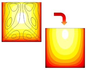
The mean streamwise velocity distributions are shown in figure 7. Due to geometrical symmetry, the maximum mean velocity in closed ducts is always located at the centre. As observed by Pirozzoli et al. (Reference Pirozzoli, Modesti, Orlandi and Grasso2018), the velocity isolines in that case tend to be parallel to the duct walls owing to the effect of the secondary motions. For the open duct cases with  ${A{\kern-4pt}R} =1$ (figure 7d–f), the presence of the free surface breaks the symmetry, making the velocity isocontours no longer closed, and shifting the maximum velocity farther from the bottom wall. In laminar open duct flows, the maximum streamwise velocity is located at the free surface, whereas in the turbulent case it dips below it, as first observed by Francis (Reference Francis1878) and Stearns (Reference Stearns1883). The mean streamwise velocity in open ducts with ${A{\kern-4pt}R} =2$, shows similar velocity dip as in the ${A{\kern-4pt}R} =1$ case (figure 7g–i). Interestingly, the mean streamwise velocity at the bottom wall in this case is rather different from the open and closed duct cases with unit aspect ratio, as the velocity isolines around the bottom wall bisector tend to bulge in opposite directions. This effect is probably due to the downwelling current from the free surface which reaches down to the bottom wall as a result of a widened free-surface as compared with the ${A{\kern-4pt}R} =1$ cases. In open ducts with ${A{\kern-4pt}R} =0.5$ (figure 7j–l) the mean streamwise velocity reaches a maximum at the deepest location amongst all cases here considered, and at the highest Reynolds number the maximum velocity is reached at approximately a distance $h$ underneath the free surface. In this case, the bulging of the velocity isolines at the bottom wall follow the typical trend found in closed ducts and for open ducts with ${A{\kern-4pt}R} =1$.

Figure 7. Mean velocity distributions  $U/u_b$, for flow cases (a) SD-L, (b) SD-M, (c) SD-H, (d) AR1-L, (e) AR1-M, ( f) AR1-H, (g) AR2-L, (h) AR2-M, (i) AR2-H, (j) AR05-L, (k) AR05-M, (l) AR05-H. The white cross denotes the position where maximum velocity is attained.
Quantitative information about the velocity maximum  $U_{max}$ is reported in table 1. The maximum velocity $U_{max}/u_b$ decreases slightly with the Reynolds number, whereas it increases when normalized in viscous units, as typical of wall turbulence. A minor difference between the various aspect ratios is that for A=2.0 the drop of $U_{max}/u_b$ seems slightly weaker for increasing Reynolds number, when compared with flow cases with ${A{\kern-4pt}R} =1$ and ${A{\kern-4pt}R} =0.5$. We note that at the highest Reynolds number the maximum velocity of the open duct case is less than for the closed duct in outer units, suggesting more efficient turbulent mixing, associated with additional momentum transfer from the secondary flows. In addition, the maximum location dips down off the free surface at increasing Reynolds number. This is in agreement with the findings of half-filled pipes by Brosda & Manhart (Reference Brosda and Manhart2022), that maximum location moves away from the free surface as the Reynolds number increases.
The mean velocity profiles taken normal to the bottom wall are shown in figure 8, at various  $z$ locations. For ducts with ${A{\kern-4pt}R} =0.5$, the velocity profiles exhibit two local maxima, the first at $y\approx h$, and the second at $y\approx 3h$, which are particularly visible at the duct centreline. The former corresponds to the maximum velocity at the edge of the bottom-wall boundary layer, whereas the second is the velocity dip near the free surface. In between these two maxima, the streamwise velocity profile shows a plateau, which becomes more evident at increasing Reynolds number. Deviations from the equilibrium law-of-the-wall (channel and pipe flow data are reported for reference) become evident towards the sidewalls, although the double peak organization is also visible away from the duct centreline. In general, agreement with the canonical law-of-the-wall is rather poor, and large deviations are observed as the sidewalls are approached. Similar result are found for ducts with different aspect ratio, the main difference being that ducts with ${A{\kern-4pt}R} =1$ and ${A{\kern-4pt}R} =2$ only have one velocity maximum near the free surface.

Figure 8. Mean velocity profiles at various  $z/h$ locations (with the increment of $0.1h$, grey lines) for flow cases with AR05-H (a,b), AR1-H (c,d), AR2-H (e, f), normalized by local viscous units (a,c,e) and global viscous units (b,d, f). Profiles at selected stations are highlighted: $z=0.25h{A{\kern-4pt}R}$ (- - - - -, blue); $z=0.5h{A{\kern-4pt}R}$ (– - – - –, green); $z=0.75h{A{\kern-4pt}R}$ (– – – –, red); $z=h{A{\kern-4pt}R}$ (——–). Symbols denote turbulent channel flow by Bernardini, Pirozzoli & Orlandi (Reference Bernardini, Pirozzoli and Orlandi2014) ( $\blacklozenge$) and turbulent pipe flow by Pirozzoli et al. (Reference Pirozzoli, Romero, Fatica, Verzicco and Orlandi2021) ( $\blacktriangle$, red) at $Re_\tau \approx 500$. The log law $u^+ = 2.44 \log (y^+)+5.2$ is shown with magenta lines (——–, pink).
In the attempt to find a simpler description of the mean velocity distribution, we build on ideas of Keulegan (Reference Keulegan1938) and Pirozzoli et al. (Reference Pirozzoli, Modesti, Orlandi and Grasso2018), who showed that velocity profiles in closed square ducts are controlled by the closest wall. In the framework of open ducts, a similar idea was advanced by Yang & Lim (Reference Yang and Lim1997) and Yang et al. (Reference Yang, Tan and Wang2012). According to those studies, flow in square and rectangular ducts features distinct flow regions, which are controlled by nearest wall, as shown in figure 9.

Figure 9. Illustration of flow regions controlled from the bottom wall (zone 1) and from the side wall (zone 2), for  ${A{\kern-4pt}R} =1$ (a), for ${A{\kern-4pt}R} =2$ (b), for ${A{\kern-4pt}R} =0.5$ (c). The dash–dotted line denotes the bottom wall bisector, whereas the dashed line denotes the corner bisector. Dotted lines indicate representative locations along which mean velocity profiles are extracted.
In figures 10 and 11 we show the velocity profiles in the two regions, as a function of the distance from the closest wall, limited to the flow cases at higher  $Re$. When plotted in this fashion, the velocity profiles close to the bottom wall (figure 10) show close similarity with the classical law-of-the-wall. The mean velocity profiles reported in this fashion agree well with the reference DNS data of plane channel flow and circular pipe flow, with a small scatter among profiles at different spanwise locations. This agreement is very good both when profiles are reported in local and in global viscous units, although the former scaling brings close universality in the vicinity of the wall, and the latter in the outer region. All the profiles show a similar logarithmic slope, although profiles in ducts with lower aspect ratio are shifted downwards, indicating reduced flow rate close to the bottom wall at matched pressure drop, which was also clear in the mean velocity contours of figure 7. Figure 11 shows the mean velocity profiles in the flow region controlled by the sidewall, at various $y/h$ locations, including at the free surface. Also in this case we find that all profiles follow the canonical law of the wall with good accuracy, the only exception being the limit profile at the free surface, probably because the wall shear stress at the mixed corner largely overshoots the mean value, which is otherwise fairly constant along the sidewall (see figure 4). Local and global wall scaling yield similar universality, although the latter yields slightly smaller scatter across the velocity profiles in the outer region.

Figure 10. Mean velocity profiles at various  $z/h$ locations ( with the increment of $0.1h$, grey lines) in the flow region controlled by the bottom wall, as a function of the wall distance (see figure 9), for flow cases AR05-H (a,b), AR1-H (c,d) and AR2-H (e, f). The profiles are scaled in local viscous units (a,c,e) and in global viscous units (b,d, f) Profiles at selected stations are highlighted: $z=0.25h{A{\kern-4pt}R}$ (- - - - -, blue); $z=0.5h{A{\kern-4pt}R}$ (– - – - –, green); $z=0.75h{A{\kern-4pt}R}$ (– – – –, red); $z=h{A{\kern-4pt}R}$ (——–). Symbols denote turbulent channel flow by Bernardini et al. (Reference Bernardini, Pirozzoli and Orlandi2014) ( $\blacklozenge$) and turbulent pipe flow by Pirozzoli et al. (Reference Pirozzoli, Romero, Fatica, Verzicco and Orlandi2021) ( $\blacktriangle$, red) at $Re_\tau \approx 500$.

Figure 11. Mean velocity profiles at various  $y/h$ locations (with the increment of $0.1h$, grey lines) in the flow region controlled by the sidewall, as a function of the wall distance (see figure 9), for flow cases AR05-H (a,b), AR1-H (c,d) and AR2-H (e, f). The velocity profiles are scaled in local viscous units (a,c,e) and in global viscous units (b,d, f). Profiles at selected stations are highlighted: $y=0.25h{A{\kern-4pt}R}$ (- - - - - -, blue); $y=0.5h{A{\kern-4pt}R}$ (– - – - –, green); $y=0.75h{A{\kern-4pt}R}$ (– – – –, red); $y=h{A{\kern-4pt}R}$ (——–); and at the free surface (– - - – - - –, orange). Symbols denote turbulent channel flow by Bernardini et al. (Reference Bernardini, Pirozzoli and Orlandi2014) ( $\blacklozenge$) and turbulent pipe flow by Pirozzoli et al. (Reference Pirozzoli, Romero, Fatica, Verzicco and Orlandi2021) ( $\blacktriangle$, red) at $Re_\tau \approx 500$.
Based on all previous observations, in figure 12 we sketch a tentative model for the structure of the secondary motions and related organization and streamwise velocity for increasing Reynolds number. The mean streamwise velocity profiles show that, with good accuracy, the flow can be regarded as made up of three nearly independent regions, controlled by the nearest wall, and the maximum velocity dips towards the duct centre at increasing Reynolds number. Therefore, in the limit of infinite Reynolds number we expect that the velocity isolines of open ducts become indistinguishable from those in a closed duct, and in both cases the asymptotic state is plug flow. Of course, close to the free-surface the flow will remain different compared with the solid walls, at any finite Reynolds number, but in an outer-units representation, such as the one of figure 7, the free-surface boundary will become visibly indistinguishable from the solid walls. This is also supported by the asymptotic boundary layer theory of Pullin, Inoue & Saito (Reference Pullin, Inoue and Saito2013), according to which in the asymptotic state of the wall layer is slip-flow with a singularity at the wall to account for the boundary condition. In open ducts the direct consequence is that the mean streamwise velocity should become symmetric, with the maximum velocity attained at the duct centre. As for the secondary flows, the Reynolds number of the present dataset is not high enough to extrapolate an asymptotic state; however, we find hints that the core circulation in open ducts will eventually become symmetric as well, with a pair of counter-rotating eddies in each corner, whose intensity saturates to a fraction of the bulk flow velocity, whereas the corner circulations become progressively more confined towards the wall.

Figure 12. Sketch of the flow organization in the cross-stream plane: (a) mean streamwise velocity and (b) stream function.
4.1. Friction
A key quantity in the design of open ducts is the friction factor. It is generally assumed (Keulegan Reference Keulegan1938; Knight et al. Reference Knight, Hazlewood, Lamb, Samuels and Shiono2018) that for the purpose of estimating the friction factor ( $\,f=8 \tau _w^*/(\rho u_b^2)$) in ducts with cross-sectional shape other than circular, the same friction formulae developed for pipe flow can be used, upon substitution of the pipe diameter with the hydraulic diameter $D_h$. Assuming that the law-of-the-wall applies at all points in the normal direction to the nearest solid wall, Pirozzoli (Reference Pirozzoli2018) found that better universality of the friction factor distribution can be achieved by using an effective hydraulic diameter $D_e$, whose general definition is
 \begin{equation} D_e = 2 y_m e^{3/2+\mathcal{C}}, \quad \mathcal{C} = \frac {y_m}A \int_0^1 P(\eta y_m) \log{\eta} \, \mathrm{d}\eta, \end{equation}
where  $\eta =y/y_m$, $y_m$ is the apothem of the duct, and $P(d)$ is the length of the locus of points at distance $d$ from the nearest wall. Equation (4.2a,b) is based on the idea that the distance from the closest wall is the controlling parameter determining the streamwise velocity and it is derived by assuming that log-law applies along a locus of points $P(d)$. In the present case of rectangular open ducts, the classical definition yields
 \begin{equation} D_h = \frac {4 L_z}{2+{A{\kern-4pt}R}}, \end{equation}
whereas (4.2a,b) yields
 \begin{align} D_e = \left\{\begin{array}{@{}ll@{}} {L_z} \, {\rm e}^{1/2-{A{\kern-4pt}R}/4} & {A{\kern-4pt}R} \le 2,\\ \dfrac{2 L_z}{{A{\kern-4pt}R}} \, {\rm e}^{1/2-1/{A{\kern-4pt}R}} & {A{\kern-4pt}R} > 2. \end{array} \right. \end{align}
Differences between the two length scales are shown in figure 13. It is clear that differences are quite small for  ${A{\kern-4pt}R} \approx 1$ ducts, whereas they become significant for shallow or tall ducts. In the flow cases under consideration, differences are at most $10$ %, for the ${A{\kern-4pt}R} =0.5$ case.

Figure 13. Variation of hydraulic diameter ( $D_h$, ——–), and effective diameter ( $D_e$, – – – –), with duct aspect ratio.
Not many data regarding the friction factor of open ducts are available in the literature, which also show some contradictory results. Experiments of open pipe flow (Ng et al. Reference Ng, Cregan, Dodds, Poole and Dennis2018) show much higher friction factor than for a filled pipe, even when the hydraulic diameter is used, whereas DNS results show good universality (Brosda & Manhart Reference Brosda and Manhart2022).
In figure 14 we plot the friction factor and the friction Reynolds number against  $Re_b$ (figure 14a,b) and $Re_{D_e}$ (figure 14c,d), for open and closed ducts (Pirozzoli et al. Reference Pirozzoli, Modesti, Orlandi and Grasso2018), along with the results of open ducts by Sakai (Reference Sakai2016), and consider Prandtl's friction formula for smooth pipes as reference,
 \begin{equation} 1/{f}^{1/2} = A \log_{10} (Re_{b} {f}^{1/2}) - B, \end{equation}
with constants  $A=2.0$, $B=0.8$. We find that DNS data for open ducts at various aspect ratios have good universality when reported in terms of $Re_b$ based on either $D_h$ or $D_e$ (namely $Re_{D_h} = u_b D_h/\nu$, $Re_{D_e} = u_b D_e/\nu$) , although some small improvement is visible when results are reported using the effective hydraulic diameter, especially for flow cases with ${A{\kern-4pt}R} =0.5$, as expected. The reference DNS data of Sakai (Reference Sakai2016) do not seem to follow Prandtl friction law well, because of the limited Reynolds number of those cases. Similar conclusions can be drawn for the friction Reynolds number.

Figure 14. Friction factor (a,c), and friction Reynolds number (b,d), as a function of bulk Reynolds number based on the hydraulic diameter (a,b), and on the effective diameter (c,d) (Pirozzoli Reference Pirozzoli2018). Symbols denote different flow cases: closed square ducts ( $\blacksquare$, blue); open square ducts ${A{\kern-4pt}R}=1$ ( $\bullet$, red); open ducts with ${A{\kern-4pt}R}=2$ ( $\blacktriangle$, orange); open ducts with ${A{\kern-4pt}R}=0.5$ ( $\blacktriangledown$, pink); open duct with ${A{\kern-4pt}R}=1$ from Sakai (Reference Sakai2016) ( $\blacklozenge$, green). Lines refer to the Kármán–Prandtl friction law.
4.2. Reynolds stresses
Spatial inhomogeneity of the flow in the  $y$ and $z$ directions gives rise to a complex distribution of the Reynolds stress tensor, $\tau _{ij}=\rho \overline {u_i u_j}$, whose components are shown in figures 15, 16 and 17 for flow cases AR1-H, AR2-H and AR05-H, respectively. The streamwise normal component $\tau _{11}$ peaks in the buffer layer near the solid walls, excluding the corner region. The minimum is instead located near the position of the maximum velocity, where production of turbulence kinetic energy is zero. As for the other two normal stresses $\tau _{22}$ and $\tau _{33}$, the intensities are stronger along the corresponding wall-normal directions, and weaker in the corresponding wall-parallel directions. At the free surface, $\tau _{22}$ is zero due to the non-penetration boundary condition, whereas the intensity of the $\tau _{33}$ component is high, especially near the bisector, which indicates intense turbulent activity right below the free surface. The turbulent shear stresses $\tau _{12}$ and $\tau _{13}$ are strong near the bottom and sidewalls, respectively, whereas the secondary shear stress $\tau _{23}$ is in comparison much weaker. The secondary shear stress is nearly negligible on the bottom and sidewalls, although it has a comparable intensity with the other components at the bottom and top corners, suggesting that its mixing action is limited to the corner regions, whereas it is not relevant close to the side and bottom walls. Similar distributions of the Reynolds stresses $\tau _{11}$, $\tau _{22}$ and $\tau _{12}$ have also been observed in the studies of Demiral et al. (Reference Demiral, Boes and Albayrak2020) and Kadia et al. (Reference Kadia, Rüther, Albayrak and Pummer2022). This general organization is found regardless of the duct aspect ratio, although characterizing differences are visible, which are due to the imprint of the secondary flows. A notable difference is for instance the bulging of the Reynolds stresses isolines for ${A{\kern-4pt}R} =2$ (figure 16) at the bottom wall, which are moulded by the strong downwelling mean motions.

Figure 15. Components of the Reynolds stress tensor in the cross-stream plane for case AR1-H: (a)  $\tau ^+_{11}$, (b) $\tau ^+_{22}$, (c) $\tau ^+_{33}$, (d) $\tau ^+_{12}$, (e) $\tau ^+_{13}$, (d) $\tau ^+_{23}$.

Figure 16. Components of the Reynolds stress tensor in the cross-stream plane for case AR2-H: (a)  $\tau ^+_{11}$, (b) $\tau ^+_{22}$, (c) $\tau ^+_{33}$, (d) $\tau ^+_{12}$, (e) $\tau ^+_{13}$, (d) $\tau ^+_{23}$.

Figure 17. Components of the Reynolds stress tensor in the cross-stream plane for case AR05-H: (a)  $\tau ^+_{11}$, (b) $\tau ^+_{22}$, (c) $\tau ^+_{33}$, (d) $\tau ^+_{12}$, (e) $\tau ^+_{13}$, (d) $\tau ^+_{23}$.
For flow cases with  ${A{\kern-4pt}R} =0.5$ we note that $\tau _{23}$ is weaker than for the other aspect ratios, and confined very close to the corners, suggesting weaker interaction among the duct walls. In this case, the distribution of $\tau _{23}$ and of the secondary flows in figure 5(h) also suggest less influence of the free surface on the turbulence organization.
These observations are consistent with our model for the mean streamwise velocity (figure 9), and we conclude that the relative importance of the free surface is determined by its relative extension compared with fluid depth, hence the influence is higher for increasing aspect ratio A. Hence it is not surprising that the flow case with  ${A{\kern-4pt}R} =0.5$, which has the smallest share of free surface compared with the overall perimeter, shows secondary flows which are quite similar to the case of a closed duct.
In figures 18 and 19 we show the normal Reynolds stress component  $\tau _{11}$ as a function of the distance from the closest wall, as in figure 9, normalized both in local and global viscous units. Both in the region close to the bottom and the sidewall, local scaling successfully yields universality of the peak streamwise velocity variance, which well matches that in pipe and channel flow. Local wall scaling also seems to yield closer similarity with pipe and channel flow in the outer region, possibly because of the interaction of the outer layer with the wall. Overall, the Reynolds stress profiles follow quite closely the data of turbulent channel and pipe flow, with the only exception of the profiles taken at the free surface, where differences are expected due to the large variation of the wall-stress at the mixed corner. Such discrepancies of the Reynolds stress at the free-surface appear to be smaller when normalized by global viscous units.

Figure 18. Streamwise Reynolds stress component at various  $z/h$ locations (with the increment of $0.1h$) in the flow region close to the bottom wall, as a function of the distance from the bottom wall (see figure 9) for flow cases AR05-H (a,b), AR1-H (c,d) and AR2-H (e, f). Profiles are scaled in local viscous units (a,c,e) and in global viscous units (b,d, f). Profiles at selected stations are highlighted: $z=0.25h{A{\kern-4pt}R}$ (- - - - -, blue); $z=0.5h{A{\kern-4pt}R}$ (– - – - –, green); $z=0.75h{A{\kern-4pt}R}$ (– – – –, red); $z=h{A{\kern-4pt}R}$ (——–). Symbols denote turbulent channel flow by Bernardini et al. (Reference Bernardini, Pirozzoli and Orlandi2014) ( $\blacklozenge$) and turbulent pipe flow by Pirozzoli et al. (Reference Pirozzoli, Romero, Fatica, Verzicco and Orlandi2021) ( $\blacktriangle$, red) at $Re_\tau \approx 500$.

Figure 19. Streamwise Reynolds stress component at various  $y/h$ locations (with the increment of $0.1h$) in the flow region close to the sidewall, as a function of the distance from the sidewall (see figure 9) for flow cases AR05-H (a,b), AR1-H (c,d) and AR2-H (e, f). Profiles are scaled in local viscous units (a,c,e) and in global viscous units (b,d, f). Profiles at selected stations are highlighted: $y=0.25h{A{\kern-4pt}R}$ (- - - - -, blue); $y=0.5h{A{\kern-4pt}R}$ (– - – - –, green); $y=0.75h{A{\kern-4pt}R}$ (– – – –, red); $y=h{A{\kern-4pt}R}$ (——–); and at the free surface (– - - – - - –, orange). Symbols denote turbulent channel flow by Bernardini et al. (Reference Bernardini, Pirozzoli and Orlandi2014) ( $\blacklozenge$) and turbulent pipe flow by Pirozzoli et al. (Reference Pirozzoli, Romero, Fatica, Verzicco and Orlandi2021) ( $\blacktriangle$, red) at $Re_\tau \approx 500$.
5. Contributions to velocity and friction
To quantitatively evaluate the role of turbulent fluctuations and secondary motions to the mean streamwise velocity field and to skin friction, we utilize the generalized form of the Fukagata–Iwamoto–Kasagi (FIK) identity introduced by Modesti et al. (Reference Modesti, Pirozzoli, Orlandi and Grasso2018), which is derived from the mean streamwise momentum equation
 \begin{equation} \nu \nabla^2 U = \left( \frac{\partial U V}{\partial y} + \frac{\partial U W}{\partial z} \right) + \left( \frac{\partial \overline{uv}}{\partial y} + \frac{\partial \overline{uw}}{\partial z} \right) - \frac{P_w \tau^*_w}{\rho A_c}, \end{equation}
with the three terms at the right-hand side representing the effects of mean cross-stream convection, turbulent convection and the mean driving pressure gradient. Accordingly, the mean velocity can be split as
 \begin{equation} U = U_C + U_T + U_V, \end{equation}
which will be referred to as the convection, turbulent and viscous velocity contributions, respectively. Due to the linearity of the Laplace operator, these are determined by solving the following Poisson equations:
 \begin{equation} \left.\begin{array}{@{}c@{}} \nu \nabla^2 U_C = \left( \dfrac{\partial U V}{\partial y} + \dfrac{\partial U W}{\partial z} \right),\\ \nu \nabla^2 U_T = \left( \dfrac{\partial \overline{uv}}{\partial y} + \dfrac{\partial \overline{uw}}{\partial z} \right),\\ \nu \nabla^2 U_V ={-} \dfrac{P_w \tau^*_w}{\rho A_c}, \end{array} \right\} \end{equation}
with homogeneous boundary conditions. The bulk velocity in the duct may accordingly be evaluated as
 \begin{equation} u_b=\frac {\tau_w^*P_w}{\rho\nu} {u_b}_1+{u_b}_T+{u_b}_C, \quad {u_b}_X = \frac{1}{A_c} \int_{A_c} U_X\,\mathrm{d}A_c, \end{equation}
where we have introduced the unitary velocity field  $u_1$ defined as solution of ${\nabla ^2 u_1 = -1/A_c}$, which by construction is only a function of the duct geometry. Hence, the viscous velocity field may be expressed as $U_V=\tau _w^*P_w u_1 / (\rho \nu )$. Inserting the friction factor ${f=8 \tau _w^*/(\rho u_b^2)}$ into (5.4a,b) one obtains
 \begin{equation} f=\frac{8}{{u_b}_1 Re_P}\left(1-\frac{{u_b}_T}{u_b}-\frac{{u_b}_C}{u_b}\right)=f_V+f_T+f_C, \end{equation}
where  $Re_P=u_b P_w / \nu$ is the bulk Reynolds number based on the duct perimeter.
The distributions of the viscous and turbulent terms are shown in figure 20, for both open and closed ducts. The viscous contribution shows the typical distribution of Hagen–Poiseuille flows (White Reference White2006). The turbulent velocity contribution is always negative, consistently with the fact that turbulent transport increases drag, and  $U_T$ depends on the Reynolds number. The effect of Reynolds number on the turbulent velocity contribution is more pronounced for the open square duct, in which the minimum velocity was seen to visibly move away from the free surface. In general, as the Reynolds number increases the isolines of $U_T$ tend to close, and the magnitude of turbulence-associated velocity at the free-surface decreases, which is consistent with the description in figure 12.

Figure 20. Contributions to mean streamwise velocity  $U$, each normalized by the corresponding bulk values, (a,c,e,g) viscous $U_V/u_{Vb}$, (b,d, f,h) turbulent $U_T/|u_{Tb}|$, of (a,b) SD, (c,d) AR1, (e, f) AR2, (g,h) AR05; flooded, L; dashed lines, M; solid lines, H. Contour levels from $-$2.0 to 2.0, in intervals of 0.2.
The contribution to the streamwise velocity from mean cross-stream convection is shown in figure 21. Both in closed and open ducts the role of mean cross-stream convection is to redistribute momentum transport across the duct cross-section by depleting the core (in closed ducts) and the free surface (in open ducts), in favour of the corners, where the velocity is lower.

Figure 21. Contribution of mean cross-stream convection term to mean streamwise velocity,  $U_C/|u_{Cb}|$: (a) SD-L, (b) SD-M, (c) SD-H, (d) AR1-L, (e) AR1-M, ( f) AR1-H, (g) AR2-L, (h) AR2-M, (i) AR2-H, (j) AR05-L, (k) AR05-M, (l) AR05-H, contour levels from $-$8.0 to 8.0, in intervals of 0.5.
The contributions of the various terms to the duct friction factor are summarized in table 2. For all cases, the primary contribution to the skin friction comes from turbulence, which increases up to 90 % at the highest Reynolds number, whereas the contribution of viscosity drops to approximately 5 %. Regarding the secondary motions, in closed ducts their contribution to the skin friction is limited to approximately 5 %, and the increment with the Reynolds number is rather slow. Secondary motions seem to play a more significant role in open ducts, as their contribution to skin friction exceeds 10 % in open ducts with  ${A{\kern-4pt}R} =1$ and ${A{\kern-4pt}R} =2$. On a final note, it seems that the contribution of convection increases substantially with the Reynolds number for all cases, supporting the fact that the intensity of the secondary flows scales with the bulk flow velocity, as we also proposed in our previous work (Pirozzoli et al. Reference Pirozzoli, Modesti, Orlandi and Grasso2018).
Table 2. Contribution of viscous, turbulent and mean cross-stream convection terms to friction factor.

6. Suppression of secondary flows
We also carried out a numerical experiment by artificially suppressing the secondary motions. For that purpose we force the streamwise-averaged cross-stream velocity components to have zero mean by setting
 $$\begin{gather} v(x,y,z,t) \rightarrow v(x,y,z,t) - \bar{v}^x(y,z,t), \end{gather}$$
 $$\begin{gather}w(x,y,z,t) \rightarrow w(x,y,z,t) - \bar{w}^x(y,z,t), \end{gather}$$
at each Runge–Kutta substep, where  $\overline {(.)}^x$ denotes the streamwise averaging operator. The method to suppress the secondary flows is rather simple and it is equivalent to adding a body force $f(y,z,t)$ to the Navier–Stokes equations which exactly suppresses the secondary flows. Therefore, the solution does not satisfy the canonical Navier–Stokes equations, but the equations with the addition of the spatial forcing. We first analyse the instantaneous flow field comparing the $u$ and $v$ velocity components for the cases with and without secondary flows, see figure 22.

Figure 22. Streamwise velocity component  $u/u_b$ (a,b) and wall-normal velocity component $v/u_b$ (c,d) in the cross-stream plane and for flow case AR1-M (a–c) and for AR1-M0 (b–d).
For flow case AR1-M, the velocity dip is evident even in the instantaneous streamwise velocity, whereas for flow case AR1-M0 it is more difficult to pinpoint the location of the maximum streamwise velocity from the instantaneous flow. It is evident that the secondary flow is responsible for a fuller streamwise velocity profile, due to the additional momentum transfer which is absent in flow case AR1-M0. We also note that in the instantaneous flow field of AR1-M, high-speed sweeps protruding towards the corner are present, whereas low momentum regions at the corner are evident for AR1-M0.
The intensity of the instantaneous wall-normal velocity component  $v$ does not seem affected by the suppression of the secondary flows, probably because the intensity of the turbulent fluctuations is approximately an order of magnitude higher than the mean cross-stream velocity components. However, we note lower coherence in $v$ for flow case AR1-M0 as a result of suppression of the large-scale structures.
Figure 23(a) shows the mean streamwise velocity in the cross-stream plane for flow case AR1-M, and AR1-M0. In the absence of secondary flows the velocity isolines are rounded, the velocity distribution is less full and the maximum velocity is higher (see table 1) because of the reduced momentum transfer. This is not sufficient to completely cancel the velocity dip, and the maximum velocity still occurs below the free surface, although much closer to it compared with flow case AR1-M. A similar conclusion can be drawn from figure 23, showing the mean velocity profile at the symmetry plane, where it is evident that the maximum velocity for flow case AR1-M0, still occurs below the free surface.

Figure 23. Mean streamwise velocity in the cross-stream plane (a) for flow case AR1-M (isolines) and for AR1-M0 (contours). The associated maximum velocity location is shown with a cross for AR1-M, and a plus for AR1-M0. In panel (b) we show the mean streamwise velocity profiles at  $z/h=0$ for flow case AR1-M (——–) and AR1-M0 (– – – –, red).
The purpose of this numerical experiment was to assess the causality link between the secondary flows and the velocity dip; however, the results are not fully conclusive, and data at much higher Reynolds number would be needed to fully clarify this point.
7. Conclusions
We have carried out DNS of square and rectangular open duct flows with aspect ratios  ${A{\kern-4pt}R} =0.5,1,2$, and up to $Re_\tau \approx 1200$, addressing several open research questions for this flow. Open-duct flow has been so far studied extensively using experiments, whereas previous simulations were limited to low Reynolds number, which left some uncertainty about the structure of the secondary flows. Using the present DNS dataset we have been able to determine precisely the topology of the secondary flows, for different Reynolds numbers and aspect ratios, and compared the results with the case of closed ducts. In agreement with previous studies, we find that secondary flows in open ducts are substantially different from those in closed ducts, featuring only four large-scale eddies instead of eight. However, we find hints of a different flow topology slowly emerging at increasingly high Reynolds number, with a large-scale circulation becoming clearly visible at the mixed-boundary corner, which is a possible hint that in the limit of very high Reynolds number the secondary flows eventually attain double symmetry. This behaviour is supported by the Reynolds number trend observed for the mean streamwise velocity. As the Reynolds number increases, the streamwise velocity peak moves away from the free surface, and the velocity isolines tend to become parallel to it, indicating that the limit state is plug flow. This limit state is consistent with the theory of Pullin et al. (Reference Pullin, Inoue and Saito2013) for high-Reynolds-number boundary layers, and also with the idea that wall turbulence is impervious to the boundary conditions, and the only role of walls is to set the wall shear stress.
The limit state that we are suggesting would imply that the velocity dip phenomenon is not due to the downwelling motion imparted by the secondary flows. To shed light on this issue, we have also carried out numerical experiments in which we have artificially suppressed the secondary flows to understand their role in the formation of the velocity dip. Suppressing the secondary flows indeed yields reduced momentum transport; however, the outcome is not fully conclusive, and data at higher Reynolds number and for different aspect ratios would be required to precisely confirm this causality link.
Friction data accurately follow Prandtl's law for circular pipe when reported with the bulk Reynolds number based on the hydraulic diameter, and slight improvement is visible when the effective diameter is used instead. The success of the hydraulic diameter is justified by the fact that the mean velocity is controlled by the closest wall, therefore the duct can be decomposed into flow regions where the standard law-of-the-wall applies. A friction decomposition based on the popular FIK identity shows that secondary flows are more important than in closed ducts and they contribute up to 15 % of the total friction factor for  ${A{\kern-4pt}R} =2$.
Although this work has shed light on some facets of flows in open ducts, several important research avenues remain open, and we believe that DNS is a powerful tool that could bring important advancement in this respect. Specifically, numerical simulations at higher Reynolds number and different aspect ratios would certainly help in clarifying some of the points we make in the paper. Additionally, flows in open ducts of different cross-section such as trapezoidal, or semicircular would certainly expand our knowledge of the subject. Finally, high-Reynolds-number simulations of more realistic configurations featuring rough walls, particle transport, or both, would contribute to transferring fundamental knowledge towards engineering design.
Acknowledgements
We acknowledge that the results reported in this paper have been achieved using the EuroHPC Research Infrastructure resource LEONARDO based at CINECA, Casalecchio di Reno, Italy, under a LEAP grant.
Funding
This research received no specific grant from any funding agency, commercial or not-for-profit sectors.
Declaration of interests
The authors report no conflict of interest.
Data availability statement
The data that support the findings of this study are openly available at the web page http://newton.dma.uniroma1.it/database/.


 Open access