


Crossref Citations
This article has been cited by the following publications. This list is generated based on data provided by Crossref.
Behera, Abhinna K.
Rivière, Emmanuel D.
Khaykin, Sergey M.
Marécal, Virginie
Ghysels, Mélanie
Burgalat, Jérémie
and
Held, Gerhard
2022.
On the cross-tropopause transport of water by tropical convective overshoots: a mesoscale modelling study constrained by in situ observations during the TRO-Pico field campaign in Brazil.
Atmospheric Chemistry and Physics,
Vol. 22,
Issue. 2,
p.
881.
Lucarini, Valerio
and
Chekroun, Mickaël D.
2023.
Theoretical tools for understanding the climate crisis from Hasselmann’s programme and beyond.
Nature Reviews Physics,
Vol. 5,
Issue. 12,
p.
744.
Cox, Michael R.
Kafiabad, Hossein A.
and
Vanneste, Jacques
2023.
Inertia-gravity-wave diffusion by geostrophic turbulence: the impact of flow time dependence.
Journal of Fluid Mechanics,
Vol. 958,
Issue. ,
Chekroun, Mickaël D
Liu, Honghu
Srinivasan, Kaushik
and
McWilliams, James C
2024.
The high-frequency and rare events barriers to neural closures of atmospheric dynamics.
Journal of Physics: Complexity,
Vol. 5,
Issue. 2,
p.
025004.
Holm, Darryl D.
Hu, Ruiao
and
Street, Oliver D.
2024.
Stochastic Transport in Upper Ocean Dynamics II.
Vol. 11,
Issue. ,
p.
111.
1. Introduction and background
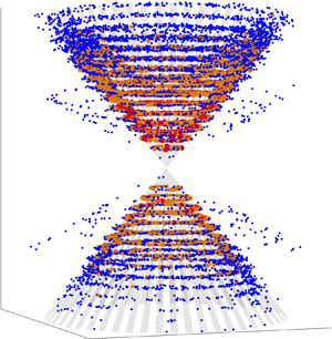
Within the rapidly rotating fluid envelope of the Earth, slow geostrophic turbulence co-exists – not entirely peacefully – with fast inertia-gravity waves (hereafter IGWs): see figure 1. Geostrophic turbulence refers to a form of two-dimensional turbulence with geophysical complications arising from density stratification and the planetary $\beta$-effect (Charney Reference Charney1971). A main departure of geostrophic turbulence from plain and simple two-dimensional turbulence is that horizontal velocities are vertically sheared. Weather systems in the atmosphere, with an evolutionary time scale of several days, are a familiar example of geostrophic turbulence. The IGWs, also known as internal waves, are higher-frequency motions that propagate vertically in a stably stratified fluid and involve a balance between inertia, buoyancy, pressure gradient and Coriolis forces. The IGW time scales are of the order of hours i.e. much shorter than those of geostrophic turbulence.
Figure 1. Co-existence of geostrophic turbulence and IGWs. The figure shows horizontal slices through a three-dimensional solution of the Boussinesq equations. The geostrophic turbulence in the lower panel is visualized by showing vertical vorticity; the IGWs in the upper panel are revealed with vertical velocity. Figure contributed by H. Kafiabad.
The interaction between waves and turbulence, with widely separated time scales, presents meteorologists and oceanographers with a ‘wave–turbulence jigsaw’ (McIntyre Reference McIntyre2008). Within the last decade, several pieces of this sprawling puzzle have quietly dropped into place. This advance has greatly clarified the extent to which there is a separation in length scale between geostrophic turbulence and IGWs. The short answer is that there is not as much separation in length scale as meteorologists and oceanographers expected: IGWs are energetic on surprisingly large scales. Geophysical kinetic energy spectra have a band of wavenumbers within which waves and turbulence are equally energetic. A painful consequence of this length-scale overlap is that the approximation of Wentzel, Kramers and Brillouin (WKB hereafter) does not apply to all scales of interest.
Separating waves from turbulence in geophysical energy spectra has required new statistical tools for the analysis of observations of fluid velocity along the one-dimensional transects made by ships and planes (Bühler, Callies & Ferrari Reference Bühler, Callies and Ferrari2014). Aircraft data show that atmospheric geostrophic turbulence dominates the synoptic range, while IGWs dominate the mesoscale range (Callies, Ferrari & Bühler Reference Callies, Ferrari and Bühler2014; Waite Reference Waite2020). The transition scale between the two ranges is at around 500 km. The oceanic situation is more complicated because the ocean is more spatially inhomogeneous than the atmosphere, and because geostrophic eddies in the ocean are much smaller than their atmospheric cousins. But the broad-brush conclusion is the same: ocean IGWs are energetic on surprisingly large length scales. For instance, Rocha et al. (Reference Rocha, Chereskin, Gille and Menemenlis2016) show that in Drake Passage, with a deformation radius of 16 km, IGWs account for roughly half of the near-surface kinetic energy at scales between 10 and 40 km.
Synthesis of oceanographic IGW data into a seemingly ‘universal spectrum’ (Garrett & Munk Reference Garrett and Munk1972) drove intensive research on nonlinear wave interactions in the seventies and eighties (Müller et al. Reference Müller, Holloway, Henyey and Pomphrey1986). While this effort did not ignore the interaction of IGWs with geostrophic turbulence – see for instance Müller (Reference Müller1976) – the focus was mainly on self-interactions within the IGW field as an explanation of the Garrett–Munk spectrum. A development driving a re-examination of the IGW spectrum is the realization that geostrophic turbulence is the main reservoir of ocean kinetic energy (Ferrari & Wunsch Reference Ferrari and Wunsch2009). The interaction of IGWs with this turbulent reservoir is likely to be an important mechanism for shaping the IGW spectrum – perhaps more important than wave–wave interactions.
2. Overview of Savva, Kafiabad & Vanneste (Reference Savva and Vanneste2021)
The recent paper by Savva et al. (Reference Savva, Kafiabad and Vanneste2021, SKV hereafter) is the first comprehensive and definitive study of IGW scattering by geostrophic turbulence. The crucial assumption of SKV is the weak-current approximation that
Here, $|\boldsymbol {U}|$ denotes the typical speed of geostrophic currents and $c_{{g}}$ is the typical group speed of IGWs. The condition (2.1) ensures that wave packets rapidly propagate through many decorrelation lengths of the turbulent velocity field and that during this passage the turbulence does not evolve significantly. Thus the scattering velocity field is effectively frozen, the Doppler shift is negligible, the intrinsic frequency of the waves is unchanged by the interaction and conservation of action (Bretherton & Garrett Reference Bretherton and Garrett1968) is, to leading order, the same as conservation of IGW energy. Because there is almost no transfer of energy between waves and turbulence the interaction is catalytic i.e. the wave field is modified by turbulence (details below) but the turbulence is unaffected by the waves. Thus SKV treats the turbulence as a random velocity field with a specified kinetic energy spectrum $E_{{K}}(\boldsymbol {k})$, where k is the wavenumber.
SKV avoids the WKB approximation by using the Wigner transform formalism of Ryzhik, Papanicolaou & Keller (Reference Ryzhik, Papanicolaou and Keller1996) and shows that the phase space energy density of the waves, denoted $a(\boldsymbol {k},\boldsymbol {x},t)$, satisfies the kinetic equation
where $\varSigma (\boldsymbol {k}) = \int \sigma (\boldsymbol {k},\boldsymbol {k}') \, \text {d} \boldsymbol {k}'$. Above $\omega (\boldsymbol {k})$ is the IGW dispersion relation
where $N$ is the buoyancy frequency and $f$ is the Coriolis frequency; the wavenumber is decomposed into horizontal and vertical components $\boldsymbol {k} = (\boldsymbol {k}_{h},k_3)$. The surface of constant $\omega$ in $\boldsymbol {k}$-space defined by (2.3) is a double cone.
The scattering cross-section in (2.2) has the form
where $\varXi (\boldsymbol {k},\boldsymbol {k}')= \varXi (\boldsymbol {k}',\boldsymbol {k})$ is given by a formidable expression in SKV. The kinetic equation (2.2) subsumes earlier studies of special cases (Danioux & Vanneste Reference Danioux and Vanneste2016; Savva & Vanneste Reference Savva and Vanneste2018; Kafiabad, Savva & Vanneste Reference Kafiabad, Savva and Vanneste2019).
The $\delta (\omega (\boldsymbol {k}') - \omega (\boldsymbol {k}))$ term in (2.4) ensures that $\omega$ is unchanged by scattering. The interaction can be viewed as a resonant triad between two IGWs and a zero-frequency geostrophic mode. The upshot is that all the IGW energy that starts on a particular constant- $\omega$ double cone stays on that same double cone. If the turbulence is horizontally isotropic then scattering of IGW energy over the surface of the $\boldsymbol {k}$-space double cone involves three processes:
(a) The horizontal rate of strain of geostrophic turbulence results in horizontal isotropization by azimuthal scattering of IGWs around the cone, with $k_h$ and $k_3$ unchanged (Savva & Vanneste Reference Savva and Vanneste2018).
(b) The vertical shear of geostrophic turbulence scatters IGW energy along the $k_3$-axis of the cone and so increases $|\boldsymbol {k}|$.
(c) Energy is weakly transferred between the two halves of the double cone via inelastic scattering (McComas & Bretherton Reference McComas and Bretherton1977).
A main result from SKV is the cascade of IGW energy to high wavenumbers in (b). The special role of vertical shear in enabling turbulent scattering to access the entire constant $\omega$ double cone is notable. This high-wavenumber IGW cascade relies on a peculiar property of the dispersion relation (2.3): the conical constant- $\omega$ surface is not compact so that scattering with constant $\omega$ can access arbitrarily high wavenumbers (The $\omega$-surface for acoustic scattering is a sphere in $\boldsymbol {k}$-space; a sphere is compact and thus turbulence cannot catalyse a cascade of acoustic energy to high wavenumbers).
As IGWs are scattered out to high wavenumbers on the cone, the WKB-based induced diffusion approximation of McComas & Bretherton (Reference McComas and Bretherton1977) becomes applicable and enables a great simplification of (2.2): the non-local transfers on the right-hand side are approximated by $\boldsymbol {k}$-space diffusion along the surface of the cone. Kafiabad et al. (Reference Kafiabad, Savva and Vanneste2019) solve this simplified version of (2.2) with analytic methods. This solution shows that induced diffusion results in a $k_h^{-2}$ spectrum of wave energy. Now $k_h^{-2}$ is a frequently observed energy spectrum in the ocean; for example, Rocha et al. (Reference Rocha, Chereskin, Gille and Menemenlis2016) show that the IGW component of the kinetic energy spectrum is $k_h^{-2}$. In the atmosphere the shallow mesoscale part of the kinetic energy spectrum is traditionally described as a $k_h^{-5/3}$ spectrum (Nastrom & Gage Reference Nastrom and Gage1985). Atmospheric data are, however, also consistent with $k_h^{-2}$. Kafiabad et al. (Reference Kafiabad, Savva and Vanneste2019) speculate that these observations in the ocean and atmosphere could be explained by the $k_h^{-2}$ spectrum resulting from induced diffusion of IGW energy by geostrophic turbulence.
3. Future
The unsteady evolution of geostrophic turbulence results in weak scattering of IGW energy off the constant- $\omega$ double cone. This cross $\omega$-surface diffusion has been demonstrated by Dong, Bühler & Shafer Smith (Reference Dong, Bühler and Shafer Smith2020) using the shallow water equations and the induced diffusion approximation. Diffusion across the $\omega$-surfaces implies an increase in wave energy, so that IGWs act as an effective viscosity on the turbulence (Müller Reference Müller1976). The next step is to investigate this effect in the Boussinesq equations and include it in the kinetic equation (2.2). In principle this can be accomplished by computing the cross- $\omega$-surface scattering as the next term in the expansion that leads to (2.2).
Another frontier is strong multiscale interactions – but not so strong as in stratified turbulence – leading to failure of (2.1). Special examples, such as the strong wave–wave interaction discussed by Broutman & Young (Reference Broutman and Young1986), show large changes in frequency and significant energy transfers. This is also likely the case for strong interactions between IGWs and geostrophic turbulence. Provided that there is a separation in length scales, this frontier problem seems approachable only via WKB and Monte Carlo simulation.
Acknowledgements
Thanks to O. Bühler, P. Cessi, H. Kafiabad and J. Vanneste for comments and discussion.
Funding
This work was supported by the National Science Foundation (award number OCE-2048583) and by the Office of Naval Research (award number N00014-18-1-2803).
Declaration of interest
The author reports no conflict of interest.