In a recent paper, Reference Campbell, Jacobel, Welch and PetterssonCampbell and others (2008) discussed the lack of correlation between the deep (>100 m) cross-flow folds in radar-detected stratigraphy and surface ‘flow stripes’. Their study focused on an area upstream of the now stagnant part of Kamb Ice Stream (KIS), West Antarctica, and they noted the lack of near-surface stratigraphy obtained by higher-frequency radar to help explain the apparent anomaly. Such data do exist and, as we illustrate below, show a good correlation between the flow-stripe image features and the near-surface stratigraphy.
Figure 1 illustrates part of the RADARSAT Antarctic Mapping Mission (AMM) 125 m mosaic and the position of two of the lines (AA’ and BB’ in figure 2 of Reference Campbell, Jacobel, Welch and PetterssonCampbell and others, 2008). These lines were also studied in the fieldwork of Reference Smith, Lord and BentleySmith and others (2002) and Reference Ng and ConwayNg and Conway (2004). The ground-penetrating radar (GPR) data used by Reference Smith, Lord and BentleySmith and others (2002) in the study of buried crevasses in the shear zone of KIS did map near-surface stratigraphy. Lines LL’ and KK’ in their figure 3 were acquired in fieldwork carried out in the 1997/98 austral summer, and correspond to the deep radar lines AA’ and BB’ of Reference Campbell, Jacobel, Welch and PetterssonCampbell and others (2008) and lines XX’and YY’ of Reference Ng and ConwayNg and Conway (2004). The choice of LL’ and KK’ by Reference Smith, Lord and BentleySmith and others (2002) reflected two of the lines used in the pioneering work of Reference Shabtaie and BentleyShabtaie and Bentley (1987).

Fig. 1. Positions of the AA’ and BB’ lines in KIS superimposed on part of the 1997 RADARSAT AMM 125 m mosaic data. The ‘flow stripes’ are typically ∼1 km wide and usually reflect the ice-flow direction.
Fig. 2. Depth to a particular isochrone (∼1951, ±4 years) versus the averaged 5.3 GHz radiometry derived from the AMM 125 m mosaic for lilnes A’A (a) and B’B (b).

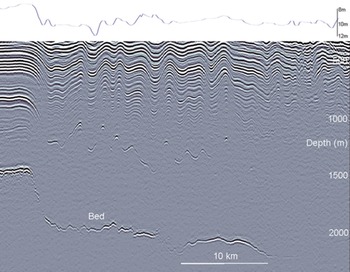
Fig. 3. Comparison of the near-surface stratigraphy (∼1951 isochronal layer, upper blue curve) obtained by Reference Smith, Lord and BentleySmith and others (2002) and the deep radar results of Reference Ng and ConwayNg and Conway (2004) for the A’A line in Figure 1.
Details of the processing of the 80 MHz Geophysical Survey Systems Inc. (GSSI) monopulse GPR are given by Reference Smith, Lord and BentleySmith and others (2002), together with the technique used to date particular layers in the stratigraphy. The depth of the firn layer deposited around 1951 (∼46 ± 4 years prior to the fieldwork) is plotted in Figure 2 for the two test lines and compared with the average 5.3 GHz radiometric variation. Radiometric smoothing of the RADARSAT data was performed primarily along the direction of the flow-stripe feature. First, the orientations of the flow stripes were estimated with respect to the two lines. Then averaging was applied with a smoothing function (∼250 × 800 m) such that the extra averaging was applied in the along-flow-stripe direction. The correlation between the depth of the particular layer and the average radiometry in Figure 2 is remarkable. Some examples of these correlations have been presented at West Antarctic Ice Sheet meetings (Conway and others, http://neptune.gsfc.nasa.gov/wais/pastmeetings/PPT04/Question3/Conway.ppt; Gray and others, http://neptune.gsfc.nasa.gov/wais/pastmeetings/PPT05/Gray.ppt; King and others, http://neptune.gsfc.nasa.gov/wais/pastmeetings/abstracts04/King.htm), including results collected during the 2000/01 British Antarctic Survey–University of Texas radar experiment over parts of Bindschadler Ice Stream and a tributary of KIS. This result appears to be general for cold polar firn in West Antarctica and does not depend on the orientation of the test line with respect to the ice motion, or the magnitude of the ice velocity. However, if the strain rates are high enough for crevasse formation then this relationship breaks down.
Figure 3 illustrates the near-surface stratigraphy studied by Reference Smith, Lord and BentleySmith and others (2002) (top curve) and the deep stratigraphy studied by Reference Ng and ConwayNg and Conway (2004). The weak correlation between the near-surface and deep stratigraphy confirms the conclusion of Reference Campbell, Jacobel, Welch and PetterssonCampbell and others (2008) that there is a weak correlation between flow stripes and deep folds. This is puzzling because, as isochrones, the near-surface stratigraphy should evolve smoothly into the deep stratigraphy.
In Figure 3 the upper 300 m of the deep radar results of line A’A are obscured by the illustration of the depth of the ∼1951 isochronal layer. Note that there is correlation between the bed and the stratigraphy (both deep and near-surface) at the left edge of the figure where the ice moves over what appears to be a subglacial escarpment. Also, there is correspondence between the near-surface and deep folds in the region vertically above the ‘Bed’ label, but otherwise the correlation is poor.
These results prompt two questions: why does the shape of cross-flow isochrones and in particular the positions of folds in the stratigraphy change with near-surface depth in a region such as the KIS? and what is the origin of the strong correlation between the RADARSAT image radiometry and near-surface stratigraphy?
The first question has been discussed in depth by Reference Campbell, Jacobel, Welch and PetterssonCampbell and others (2008), and we make only the following comments: Near-surface stratigraphy (to ∼10 m) is controlled largely by accumulation which varies locally, depending primarily on surface slope and prevailing winds. But the surface slope is itself influenced by forces acting on the ice and firn, including those that reflect movement over the varied basal topography and other conditions. Also, with time (and depth), isochrone separation becomes more a function of the cumulative history of the strain than of the original accumulation. For example, if the firn in a region of creep or tributary flow undergoes a relatively modest horizontal strain of 10−3 a1 in the flow direction, and zero across-flow, then the associated vertical GPR stratigraphy will decrease by ∼10% in only 100 years. Remembering that it takes many hundreds of years to accumulate 100 m of firn in this region of West Antarctica, and that deeper layers originated further and further upstream, the deeper folds reflect the accumulated strain history much more than the original spatial accumulation pattern. We believe this to be particularly true in this region where the forces, and the resulting strain history, may be complex (large changes in ice thickness, basal drag, and ice-flow speed and direction). While any discussion of the origin of the flow stripes is beyond the scope of this correspondence, we do note that they appear to originate in KIS downstream from a relatively large change in bed topography. Also, the increasing amplitude of the folds with depth and the downstream compression of the observed patterns (Reference Ng and ConwayNg and Conway, 2004) imply that lateral compression is a key component in the generation of the folds. Considering the more brittle nature of the cold upper firn layers, it is perhaps not surprising that the shape of the near-surface folds, and the resulting flow-stripe pattern, may not be preserved in the deep folds.
Secondly, why is there such a strong correlation between the RADARSAT image radiometry and near-surface stratigraphy? The first important point is that the 5.3 GHz radiometric variations in interior West Antarctica reflect a strong volume component to the backscatter; radiometric contrast across flow stripes is greater than that which could arise from backscatter variation with surface slope alone. Also, biases between airborne interferometric synthetic aperture radar (InSAR) and laser-derived topography over ice sheets (Reference Dall, Madsen, Keller and ForsbergDall and others, 2001; Reference Rignot, Echelmeyer and KrabillRignot and others, 2001) demonstrate the importance of subsurface volume backscatter in 5.3 GHz SAR data in cold polar firn, and of the effective depth (∼10 m) from which the integrated backscatter originates.
But what physical structures in the upper ∼10 m of the cold polar firn contribute to the modulation in the back-scatter signal? The strong correlation between the 50– 100 MHz near-surface GPR results and the off-nadir 5.3 GHz imagery suggests that the source of the variability may be the same for both radar observations. Reference Arcone, Spikes, Hamilton and MayewskiArcone and others (2004), using a 400 MHz GPR, provide evidence that thin ‘wind-crust’ ice layers (1–2 mm thick, often associated with widespread hoar-frost events) act as reflectors and that the integrated response from these dielectric discontinuities could lead to the stratigraphic modulations in the near-surface GPR results. Note that the link to widespread meteorological conditions satisfies the requirement that the resulting modulation would be isochronal over relatively large distances. During the formation of the thin ice layers they reflect the current shape of the surface and, as such, have a roughness and dielectric constant discontinuity such that the integrated response from many such layers could also contribute significantly to off-nadir 5.3 GHz backscatter. The increased 5.3 GHz radiometric brightness associated with the peaks (shorter delay time) in the GPR stratigraphy could simply reflect the fact that there would be more ice layers per meter of depth in the lower-accumulation regions than in the higher-accumulation areas. If this explanation proves credible then it may also be instrumental in explaining the empirical correlation between accumulation and space-borne scatterometer (e.g. Reference Drinkwater, Long and BinghamDrinkwater and others, 2001) and radiometer signatures (e.g. Reference Arthern, Winebrenner and VaughanArthern and others, 2006).
Acknowledgements
The RADARSATAMM was a joint Canadian Space Agency – NASA project led by K. Jezek, of The Ohio State University, USA. We thank N. Lord and T. Gades for help in the 1997/98 fieldwork. The formation of ‘wind-crust ice layers’ in polar firn and the link to hoar-frost layers was discussed with the late R. Koerner and M. Demuth of the Geological Survey of Canada. Their help is gratefully acknowledged.
12 September 2008