


Upon further examination, we have determined that the streamline patterns in figure 3 of Basu & Stremler (Reference Basu and Stremler2017) are not shown in the co-moving frame as intended; the identical error was also made in figure 4(C–F) of Basu & Stremler (Reference Basu and Stremler2015) and figure 3.3(C–F) of Basu (Reference Basu2014). The vortex positions and strength ratios used in these figures do correctly correspond to equilibrium configurations that translate uniformly without relative motion, but the equations used to generate the corresponding flow patterns contained an error that resulted in streamlines being determined in a frame of reference for which the vortices move uniformly instead of remaining stationary. The equations governing passive particle motion, which were not included in these publications, are shown here for clarity.
The motion of a passive particle at  $z=x +\textrm {i}y$ that is being advected by $N$ point vortices with strengths $\varGamma _{\alpha }$ at positions $z_{\alpha } = x_{\alpha } +\textrm {i}y_{\alpha }$ in a periodic strip of width $L$ is given by
 \begin{equation} \frac{\textrm{d}{z^{\ast}}}{\textrm{d}{t}} = \frac{1}{2L{\textrm{i}}}\sum_{\alpha=1}^{N} \varGamma_{\alpha} \cot\left[\frac{\rm \pi}{L}(z - z_{\alpha})\right], \end{equation}
where the asterisk indicates complex conjugation. The equations of motion for this particle can be written in Hamiltonian form as
 \begin{gather} \frac{\textrm{d}{z^{\ast}}}{\textrm{d}{t}} = \textrm{i} \frac{\partial{\mathcal{H}_p}}{\partial{z}}, \end{gather}
 \begin{gather}\mathcal{H}_p(z,t) = - \frac{1}{2{\rm \pi}} \sum_{\alpha=1}^{N} \varGamma_{\alpha} \ln\left\{ \sin\left[ \frac{\rm \pi}{L} \left( z - z_{\alpha}(t) \right) \right] \right\}, \end{gather}
where  $\mathcal {H}_p$ is the complex continuation of the real-valued Hamiltonian function, $H_p = \textrm {Re}(\mathcal {H}_p)$. If, as is the case in Basu (Reference Basu2014) and Basu & Stremler (Reference Basu and Stremler2015, Reference Basu and Stremler2017), the vortices are positioned such that they form a relative equilibrium configuration translating only in the ${\pm } x$ direction, then they move uniformly with real-valued speed
 \begin{equation} U = \frac{1}{2L{\textrm{i}}}\sideset{}{'}\sum_{\beta=1}^{N} \varGamma_{\beta} \cot\left[\frac{\rm \pi}{L}(z_{\alpha} - z_{\beta})\right] \end{equation}
for every choice of  $\alpha \in \{1,\ldots , N\}$; the prime in (3) indicates that the sum omits the singular term $\alpha =\beta$. One can then consider the fluid motion in the co-moving frame with coordinates $\hat {z} = \hat {x} +\textrm {i} \hat {y}= z- Ut$, in which the vortices remain stationary at positions $\hat {z}_{\alpha } = z_{\alpha } - U t$. Since we are assuming $U$ is real valued, we trivially have $y = \hat {y}$. In this co-moving frame, the Hamiltonian system becomes
 \begin{gather} \frac{\textrm{d}{\hat{z}^{\,\ast}}}{\textrm{d}{t}} = \textrm{i} \frac{\partial{\hat{\mathcal{H}}_p}}{\partial{\hat{z}}}, \end{gather}
 \begin{gather}\hat{\mathcal{H}}_p(\hat{z}) = - \frac{1}{2{\rm \pi}} \sum_{\alpha=1}^{N} \varGamma_{\alpha} \ln\left\{ \sin\left[ \frac{\rm \pi}{L} \left( \hat{z} - \hat{z}_{\alpha} \right) \right] \right\} + \textrm{i} U \hat{z}. \end{gather}
In Basu (Reference Basu2014) and Basu & Stremler (Reference Basu and Stremler2015, Reference Basu and Stremler2017), the coefficient of the first term in (4b) was erroneously taken to be  $-1/4{\rm \pi}$, which effectively caused the streamlines to be given in a frame translating with speed $2U$ instead of $U$. In terms of the Hamiltonian $\hat {H}_p = \textrm {Re} (\hat {\mathcal {H}}_p )$ or the streamfunction $\hat {\psi }$, the velocity at a point in the field of the stationary vortices in the co-moving frame is given by
 \begin{equation} \frac{\textrm{d}{\hat{x}}}{\textrm{d}{t}} = \frac{\partial{\hat{H}_p}}{\partial{\hat{y}}} = \frac{\partial{\hat{\psi}}}{\partial{\hat{y}}}, \quad \frac{\textrm{d}{\hat{y}}}{\textrm{d}{t}} = -\frac{\partial{\hat{H}_p}}{\partial{\hat{x}}} = -\frac{\partial{\hat{\psi}}}{\partial{\hat{x}}}. \end{equation}
The streamfunction  $\hat {\psi }$ in the co-moving frame is equivalent to $\hat {H}_p$ within an additive constant, so level curves of $\hat {H}_p$ give steady streamlines in the field of the stationary vortices located at positions $\hat {z}_{\alpha }$. Representative streamlines in the appropriate co-moving frame for the $N=4$ relative equilibrium configurations considered in Basu (Reference Basu2014) and Basu & Stremler (Reference Basu and Stremler2015, Reference Basu and Stremler2017) are shown in figures 1 and 2; the panels in figure 1 should replace panels (C–F) in figure 3.3 of Basu (Reference Basu2014) and figure 4 of Basu & Stremler (Reference Basu and Stremler2015), and figure 2 should replace figure 3 of Basu & Stremler (Reference Basu and Stremler2017). By taking $\mathbb {S}=\varGamma _1+\varGamma _2 > 0$ as the characteristic vortex strength, the dimensionless translational velocity of these equilibrium configurations (in a fixed frame) can be written as $\mathcal {U}=UL/\mathbb {S}$.

Figure 1. Relative equilibrium vortex configurations with glide-reflective symmetry and representative streamlines on the  $(x,y)$-plane in a reference frame co-moving with the vortices for parameter choices $\gamma =2/5$ and $\mathcal {P} = -1$; panels are labelled as in figure 3.3(C–F) from Basu (Reference Basu2014) and figure 4(C–F) from Basu & Stremler (Reference Basu and Stremler2015). Representative vortices are labelled according to their (relative) strength. Each of these relative equilibrium configurations translates steadily with respect to a fixed frame with speed (C) $\mathcal {U} \approx -0.247$, (D) $\mathcal {U} \approx -0.100$, (E) $\mathcal {U} \approx -0.501$ and (F) $\mathcal {U} \approx -0.165$. The $x$ and $y$ axes are all shown to the same scale.

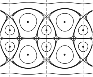
Figure 2. Relative equilibrium vortex configurations with reflective symmetry and representative streamlines on the  $(x,y)$-plane in a reference frame co-moving with the vortices for parameter choices $\gamma =3/7$ and $\mathcal {P} = -1$; panels are labelled as in figure 3 from Basu & Stremler (Reference Basu and Stremler2017). Representative vortices are labelled according to their (relative) strength. Each of these relative equilibrium configurations translates steadily with respect to a fixed frame with speed (C) $\mathcal {U} \approx -0.209$, (D) $\mathcal {U} \approx -0.071$, (E) $\mathcal {U} \approx -0.520$ and (F) $\mathcal {U} \approx -0.377$. The $x$ and $y$ axes are all shown to the same scale.
Declaration of interests
The authors report no conflict of interest.


