


1. INTRODUCTION
Monitoring of mass changes in Antarctica has become an important research topic because melting of the Antarctic ice sheet (AIS) and the resulting discharge contribute significantly to changes in the sea level (Bamber and others, Reference Bamber, Riva, Vermeersen and LeBroq2009b; Cazenave and Llovel, Reference Cazenave and Llovel2010; Shepherd and others, Reference Shepherd2012; Vaughan and others, Reference Vaughan and Stocker2013). The contribution of changes in the polar ice sheet to rising sea levels displays an accelerating trend compared with changes in the other two major contributors: continental glaciers and expansion of seawater caused by higher temperatures (Domingues and others, Reference Domingues2008; Chen and others, Reference Chen, Wilson, Blankenship and Tapley2009; Cazenave and Llovel, Reference Cazenave and Llovel2010; Rignot and others, Reference Rignot, Velicogna, van den Broeke, Monaghan and Lenaerts2011a; Zwally and Giovinetto, Reference Zwally and Giovinetto2011). Both its vast ice mass and its increasing rate of change make observations of the AIS a high priority. Furthermore, the potential instability of the ice sheet due to effects related to accelerated ice flow, subsurface lakes and basal ice-shelf melting may significantly affect the overall rate of change, and the ice sheet needs to be closely monitored and modeled using regional and local observations (Ivins, Reference Ivins2009; Flament and others, Reference Flament, Gurnis and Muller2013; Moholdt and others, Reference Moholdt, Padman and Fricker2014; Liu and others, Reference Liu2015; Paolo and others, Reference Paolo, Fricker and Padman2015).
Analysis of changes in the AIS can be performed using remote-sensing technologies, including among others, mass change measurements from satellite gravimeters and surface elevation measurements from satellite altimeters. Satellite gravimeters quantify the total mass variations produced by variations in all layers underlying the remote-sensing footprint. The major missions providing satellite gravimeter data started with Challenging Mini-satellite Payload (CHAMP) in 2000 (Reigber and others, Reference Reigber, Lühr and Schwintzer2002a), followed by Gravity Recovery and Climate Experiment (GRACE) in 2002 (Tapley and others, Reference Tapley, Bettadpur, Watkins and Reigber2004a) and Gravity Field and Steady State Ocean Circulation Explorer (GOCE) in 2009 (Drinkwater and others, Reference Drinkwater, Floberghagen, Haagmans, Muzi, Popescu and Beutler2003). One major goal of the CHAMP mission was to improve knowledge of the Earth's gravity field (Reigber and others, Reference Reigber2002b). In this mission, the low precision resulted in insufficient data concerning time-variable components of the gravity field. GOCE was specifically designed to measure the static gravity field (geoid and gravity anomalies) with high accuracy and spatial resolution (Rummel and others, Reference Rummel, Balmino, Johannessen, Visser and Woodworth2002). The GRACE mission launched a set of twin satellites on 17 March 2002. These satellites have been collecting detailed monthly measurements of Earth's gravity field at a resolution of ~400 km and an accuracy of ~1.5 cm (1σ) w.e. height at spatial scales >~800 km, and the measurements include those in Antarctica (Wahr and others, Reference Wahr, Swenson, Zlotnicki and Velicogna2004; Chen and others, Reference Chen, Wilson, Blankenship and Tapley2006).
In contrast to gravimeters, satellite altimeters directly measure ice-sheet surface elevations. Radar altimetry technology was realized in European Remote-Sensing (ERS) missions ERS-1 and ERS-2, which completed operations in 2000 and 2011, respectively (Davis, Reference Davis1992). Another radar altimeter aboard the Envisat (Environmental Satellite) mission operated from 2002 to 2010 (Rémy and Parouty, Reference Rémy and Parouty2009; Memin and others, Reference Memin, Flament, Rémy and Llubes2014). The Ice, Cloud and Land Elevation Satellite (ICESat) and Earth Explorer Opportunity Mission-2 (CryoSat-2) missions have been supplying laser and radar altimetric data on the vertical changes in the surface of Antarctica from 2003 to the present (Drinkwater and others, Reference Drinkwater, Francis, Ratier and Wingham2004; Schutz and others, Reference Schutz, Zwally, Shuman, Hancock and DiMarzio2005; Wingham and others, Reference Wingham2006a; McMillan and others, Reference McMillan2014), with a short gap from 2009 to 2010 that can be partially filled with data from NASA's Operation IceBridge (Koenig and others, Reference Koenig, Martin, Studinger and Sonntag2010). The ICESat mission acquired valuable data on elevation changes in the Greenland ice sheet (GIS) and AIS between 2003 and 2009 using its geoscience laser altimeter system (GLAS) (Zwally and others, Reference Zwally2002). The GLAS/ICESat included a 1064 nm laser channel for surface altimetry and was designed for a range measurement precision of 10 cm. It achieved an accuracy (1σ) of 14 cm in its surface elevation measurements (Schutz and others, Reference Schutz, Zwally, Shuman, Hancock and DiMarzio2005; Shuman and others, Reference Shuman2006; Shepherd and others, Reference Shepherd2012). A better accuracy (1σ) of 5 cm was achieved under optimal conditions (Fricker and others, Reference Fricker2005; Moholdt and others, Reference Moholdt, Nuth, Hagen and Kohler2010).
The GRACE and ICESat missions were expected to provide advanced time series data on changes in the AIS. A comparison of the secular mass changes in the AIS derived from the two independent GRACE and ICESat datasets over a period from 2003 to 2007 indicated a correlation between the two (Gunter and others, Reference Gunter2009). Ewert and others (Reference Ewert, Groh and Dietrich2012) presented a similar approach to a comparative study of mass changes in the GIS from 2003 to 2008 that were estimated from GRACE and ICESat data. The derived mass changes indicated a consistent overall rate of change in the GIS when an appropriate firn density was chosen, whereas the change rates in individual basins appear to feature lower degrees of agreement. A similar study on the estimation of Antarctic height and mass change rates was introduced by Memin and others (Reference Memin, Flament, Rémy and Llubes2014) using Envisat radar altimetry data for 2003–2010. A reconciled estimate of the ice-sheet mass balance using a variety of remote sensing and in situ observations, including GRACE and ICESat data, was reported by Shepherd and others (Reference Shepherd2012).
This study focuses on regional ice-sheet changes in the Lambert Glacier/Amery Ice Shelf system (LAS), East Antarctica. As illustrated in Figure 1, the LAS study area (red wedge) is located in the region of 66.5–81°S and 40–95°E, covering an area of 2 427 820 km2. This region was extended from the LAS area (68.5–81°S and 40–95°E) defined by Fricker and others (Reference Fricker, Warner and Allison2000) to include four tributary basins (Basins 2, 3, 5 and the most of Basin 4 in Fig. 1) contributing to the mass balance of the Amery Ice Shelf. The LAS is the largest glacier/ice shelf system in East Antarctica.
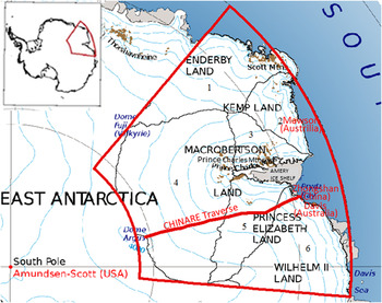
Fig. 1. Study area (red wedge) of LAS, 66.5–81°S and 40–95°E, modified from an Antarctica Overview Map produced by LIMA (2012). The red outline indicates the CHINARE traverse from Zhongshan station to Dome A. Accumulation basins, 1–6 are labeled.
The area of the grounded portion of the LAS is ~16% of the East AIS (Fricker and others, Reference Fricker, Warner and Allison2000). Although change in areal extent is not directly related to change in the mass balance in Antarctica, the two are linked (Foley and others, Reference Foley, Ferrigno, Swithinbank, Williams and Orndorff2013). Table 1 lists published estimates of the trends in mass changes in the LAS from 1992 to 2013 using various data and methods. Certain publications have presented estimated mass changes for all of Antarctica and specific changes at the basin level. Others have used basins defined by various boundaries and presented differences for comparison. We recalculated the mass change rates in the LAS and surroundings in our study area, illustrated in Figure 1, based on published results (Table 1). Our recalculation used an area-based adjustment method that is explained in the Supplementary Material.
Table 1. Trends in the mass change estimates for the LAS from 1992 to 2013 by different authors

The first two estimated trends for the LAS in Table 1 by Zwally and others (Reference Zwally2005) and Wingham and others (Reference Wingham, Shepherd, Muir and Marshall2006b) span the period, 1992–2003 and used the long-term observations of the ERS-1 and -2 radar altimeters. The recalculated trends in the LAS were based on the results for the entire Antarctica. The results reached the opposite trends of −13 ± 7 Gt a−1 for 1992–2001 and 14 ± 1 Gt a−1 for 1992–2003 in the LAS. Zwally and Giovinetto (Reference Zwally and Giovinetto2011) compared the two opposite ERS-based estimates for the entire AIS. Among the differences discussed, the factors that may have caused the different regional estimates in the LAS include the firn density and data coverage in the high slope coastal region. Zwally and others (Reference Zwally2005) considered the mass changes of 1992–2001 as a long-term imbalance and used a density of 900 kg m−3 for the firn/ice column. A firn compaction correction using the firn temperature was also applied. Considerations of the elevation changes in the upper firn layers or the whole firn/ice column were given by Wingham and others (Reference Wingham, Shepherd, Muir and Marshall2006b) to reach a preferred estimate. Corrections for accumulation anomalies in 1992–2001 determined from atmospheric modeling were applied. No conclusive suggestion was given by Zwally and Giovinetto (Reference Zwally and Giovinetto2011) for a choice between the two estimates for the AIS. Although we also cannot favor either estimate, the available in situ density measurements along the CHINARE traverse can be applied to analyze the effect of the density uncertainty on the altimetry-based trend estimation.
Ren and others (Reference Ren, Allison, Xiao and Qin2002) performed a study of the LAS. An increase of 17 Gt a−1 during the period, 1994–1999 was estimated from in situ measurement data of ice flow speed and accumulation. These data were obtained using GPS measurements and bamboo stakes along a Chinese expedition route (CHINARE traverse in Fig. 1) and an Australian ANARE expedition route. No exact study area boundary or error estimate was presented.
Rignot and others (Reference Rignot2008) used InSAR data and snow accumulation data to estimate the Antarctic mass change in 2000, while Yu and others (Reference Yu, Liu, Jezek, Warner and Wen2010) performed another study specifically for the LAS in 2000 based on RADARSAT images, snow accumulation and in situ observations. Again, the two recalculated trends for the LAS in 2000 are opposite, −14 ± 25 Gt a−1 by Rignot and others (Reference Rignot2008) and 42 ± 8 Gt a−1 by Yu and others (Reference Yu, Liu, Jezek, Warner and Wen2010). In this case, the period and the speed information are both from InSAR data. However, one of the important information sources used in the computations is the snow accumulation data. The mass-balance study of Yu and others (Reference Yu, Liu, Jezek, Warner and Wen2010) was specifically for the LAS. The regional accumulation was determined by using the accumulation data interpolated from in situ observations and the tributary sub-basin boundaries that were specifically remapped from ICESat data and satellite images. Its positive trend is also in line with the published estimates of more recent years.
King and others (Reference King2012) estimated an Antarctic mass balance based on GRACE data from 2002 to 2010 using the W12a GIA model (a glacial isostatic adjustment (GIA) model), and we recalculated an estimated regional LAS trend of 36 ± 11 Gt a−1. Furthermore, a positive trend of 35 ± 8 Gt a−1 in the LAS during the period of 2003–2012 was recompiled from Antarctic results from GRACE data published by Sasgen and others (Reference Sasgen2013). These two estimates from the GRACE data during a largely overlapping period are consistent in the LAS.
Based on CryoSat-2 data spanning the period, 2010–2013, a smaller estimated increase of 2 ± 18 Gt a−1 was obtained from the Antarctic results of McMillan and others (Reference McMillan2014).
The first five estimated trends in the LAS in Table 1 are from 1999 to 2003, and were derived from the earlier satellite radar altimetry and InSAR observations and ground measurements. The significant discrepancies may be mainly attributed to the lack of regional knowledge such as the firn density distribution and high-quality accumulation, which are important for the methods based on altimetry data and regional input/output information. The three more recent trends from 2002 to 2013 in Table 1 were estimated from the GRACE and CryoSat-2 data and showed consistently positive trends, which are partly in line with the overall positive trend of 26 ± 36 Gt a−1 in East Antarctica from 2000 to 2011, which was estimated by reconciling results from gravimetry, altimetry and input/output methods (Shepherd and others, Reference Shepherd2012). Furthermore, there seems to be a difference in the positive trend magnitude in the LAS between the longer-term estimate of 36 ± 11 Gt a−1 (2002–2010; GRACE) and the shorter-term estimate of 2 ± 18 Gt a−1 (2010–2013; CryoSat-2). It is valuable to perform a systematic investigation by using overlapping satellite and in situ observations in the LAS to contribute to the understanding of the regional dynamics.
The objectives of this study were: (1) to evaluate and compare the mass change rates in the LAS region based on GRACE and ICESat data from 2004 to 2008, and (2) to use in situ CHINARE observations, in the context of previous studies, to improve the regional estimates and to help resolve discrepancies in LAS mass change estimates. In the following sections, the methodologies used for the GRACE and ICESat regional data processing were introduced. Trend estimates and spatial variations were achieved in both the LAS region and its individual basins. The elevation change rate derived from the ICESat data was compared with the height change (accumulation) rate calculated from the snow-stake data collected along the CHINARE expedition traverse. GIA corrections and the in situ measurements of the firn density of CHINARE were taken into account before the comparative analysis. Discussions and conclusions are drawn in the later sections.
2. MASS CHANGE ESTIMATION FROM GRACE OBSERVATIONS
2.1. GRACE data processing method
The officially released RL05 GRACE monthly gravity field models are available on the website of the International Centre for Global Earth Models (http://icgem.gfz-potsdam.de/ICGEM/). Other contributing GRACE monthly models, including the Tongji-GRACE01 model (Chen and others, Reference Chen2015a, Reference Chen, Shen, Zhang, Chen and Hsub), are also available on the same website. Using elastic loading theory (Farrell, Reference Farrell1972), the Stokes coefficients can be used to calculate a surface mass anomaly Δσ at a location (Wahr and others, Reference Wahr, Molenaar and Bryan1998) using the expression
 $$\eqalign{\Delta \sigma (\theta, \lambda ) & = \displaystyle{{a{\rho _{{\rm ave}}}} \over 3}\sum\limits_{l = 0}^{{N_{\max}}} {\sum\limits_{m = 0}^l {\displaystyle{{2l + 1} \over {1 + {k_l}}}{{\bar P}_{lm}}({\rm cos}\theta )}} \cr & \quad \times (\Delta {C_{lm}}{{\rm \cos} (m\lambda ) + \Delta {S_{lm}}{\rm sin}(m\lambda )),}} $$
where θ and λ are the colatitude and longitude; a is the semimajor radius of the Earth; ρ
ave is the average density of the Earth (5517 kg m−3); ${\bar P_{lm}}({\rm cos}\theta )$
is the normalized associated Legendre function; k
l
is the lth Love number; ΔC
lm
and ΔS
lm
are the time-variable Stokes coefficients with l and m being the degree and order, respectively; and N
max is the maximum degree of the time-variable gravity solution from the GRACE measurements.
${\bar P_{lm}}({\rm cos}\theta )$
is the normalized associated Legendre function; k
l
is the lth Love number; ΔC
lm
and ΔS
lm
are the time-variable Stokes coefficients with l and m being the degree and order, respectively; and N
max is the maximum degree of the time-variable gravity solution from the GRACE measurements.
Estimates of the monthly mass changes are the basic information used to calculate the mass change rate. Suppressing noise in the monthly GRACE data is important for the reliability of the mass change analysis. Much of the spatial noise in the surface mass change fields derived from the GRACE data, which are represented as north/south-oriented stripes, is caused by correlations among estimated spherical harmonics, with extra noise increasing with the spherical harmonic degree (Swenson and Wahr, Reference Swenson and Wahr2006). We eliminated these inter-coefficient correlations using a two-step filtering procedure. The first step involves the method of Chen and others (Reference Chen, Wilson, Tapley and Grand2007, Reference Chen, Wilson, Blankenship and Tapley2009), which removes the correlation noise at spherical harmonic orders of eight or more. This method fits a third-order polynomial to a set of even or odd coefficients corresponding to each order. Then, the polynomial is subtracted from the coefficients. This method is referred to as P3M8 and has been proved to be effective in reducing noise and preserving geophysical signals (Liu, Reference Liu2008; Zhao and others, Reference Zhao2011). The second step involved applying an anisotropic Fan filter with averaging radii of 300 km to both the degree and order (Zhang and others, Reference Zhang, Chao, Lu and Hsu2009; Tang and others, Reference Tang, Cheng and Liu2012) with the goal of suppressing any remaining noise in the monthly anomalies. After the Fan filtering functions W l and W m are introduced, Eqn (1) is rewritten (Wahr and others, Reference Wahr, Molenaar and Bryan1998; Luo and others, Reference Luo, Li, Zhang and Wang2012) as follows:
 $$\eqalign{\Delta \sigma (\theta, \lambda ) & = \displaystyle{{a{\rho _{{\rm ave}}}} \over 3}\sum\limits_{l = 0}^{{N_{\max}}} {\sum\limits_{m = 0}^l {\displaystyle{{2l + 1} \over {1 + {k_l}}}{{\bar P}_{lm}}({\rm cos}\theta ){W_{l,m}}}} \cr & \quad \times (\Delta {C_{lm}}\cos (m\lambda ) + \Delta {S_{lm}}{\rm sin}(m\lambda )),} $$
where W l,m = W l × W m . W l and W m are recursively calculated using the equations W l+1 = −(2l + 1/b)W l + W l−1 and W m+1 = −(2l + 1/b)W m + W m−1 based on the initial values of W 0 = 1, W 1 = −(1 + e −2b /1 − e −2b ) − (1/b) and b = ln(2)/(1 − cos(r/a)). The variable r is the radius of the Fan filtering (Jekeli, Reference Jekeli1981; Zhang and others, Reference Zhang, Chao, Lu and Hsu2009) and was set to a value of 300 km based on the resolution of the Center for Space Research (CSR solutions).
In the CSR RL05 data, SLRF2005/LPOD2005, which is consistent with ITRF2005, was used. The mass density change Δσ(θ, λ) was converted to a change in the equivalent water height (EWH), Δh(θ, λ), by dividing by the density of water. This method for processing the GRACE data can be applied to the entire Earth. However, there are some special considerations when applied to Antarctica. For example, Figure 2 shows the estimated global cumulative mass density anomalies from February 2006 to October 2006, which were estimated using the monthly gravity field solutions (GSM coefficients or GRACE Stokes coefficients as denoted by the GRACE project) with the inserted degree-one coefficients (Fig. 2a) and from the GSM without the degree-one coefficients (Fig. 2b). Adding the degree-one coefficients notably changes the gravity anomaly values, especially in Antarctica. For implementation, the geocenter parameters were obtained from ftp.csr.utexas.edu/pub/slr/geocenter/ (Chen and others, Reference Chen, Wilson, Tapley, Blankenship and Young2008) and the terms were calculated by using equations from Barletta and others (Reference Barletta, Sørensen and Forsberg2013).

Fig. 2. Global cumulative mass density anomalies (EWH) (m) derived from GRACE data from February 2006 to October 2006: (a) estimate using GSM with inserted degree-one coefficients and (b) estimate using GSM without degree-one coefficients.
Figure 3 shows the results of the two-step processing of the inter-coefficient correlation removal and filtering. The annual mass anomaly in Antarctica from February 2004 to February 2005, calculated from the monthly GRACE data solutions via least squares fitting, exhibits meridional stripes in Figure 3a. These stripes were attenuated in Figure 3b after the P3M8 decorrelation. In another example, the residual noise after the application of the P3M8 decorrelation to the mass anomaly from October 2004 to February 2005 remains significant when filtered by a Gaussian filter with a window size of 500 km (Fig. 3c). However, the Fan filter with a window size of 300 km is effective in removing the noise (Fig. 3d).
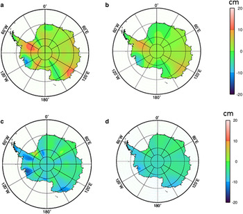
Fig. 3. Effectiveness of inter-coefficient decorrelation and Fan filtering: (a) annual mass anomaly of Antarctica from February 2004 to February 2005 computed from GRACE data, (b) meridional stripes removed by P3M8 decorrelation; (c) mass anomaly (after P3M8 decorrelation) from October 2004 to February 2005 with significant residual noise filtered by a Gaussian filter, and (d) mass anomaly results using a Fan filter instead of a Gaussian filter.
Corrections for atmospheric and oceanic effects are performed by the GRACE Project, and these signals were removed from the level-one data released by the GRACE processing centers (Bettadpur, Reference Bettadpur2007a, Reference Bettadpurb; Swenson and others, Reference Swenson, Chambers and Wahr2008; Velicogna and Wahr, Reference Velicogna and Wahr2013). Velicogna and Wahr (Reference Velicogna and Wahr2013) indicated that the residual errors due to atmospheric effects in the released GRACE data are negligible with regard to mass-balance estimates of the entire ice sheet. We did not perform any additional atmospheric corrections.
A GIA was applied, which corrects for the overall upward rebound movement caused by the post-glacial recovery in Antarctica (Nakada and others, Reference Nakada2000; Ivins and James, Reference Ivins and James2005). GIAs have been used in many applications, such as crustal movement (mainly in the vertical direction), sea-level change, gravity fields, earth rotation and earth stress (Lambeck, Reference Lambeck1977; Sabadini and Vermeersen, Reference Sabadini and Vermeersen2004; Wang and others, Reference Wang, Wu and Xu2009; Yamamoto and others, Reference Yamamoto, Yoichi and Koichiro2010). Three GIA models are used in this study – the Paulson 2007 (Paulson and others, Reference Paulson, Zhong and Wahr2007), W12a (Whitehouse and others, Reference Whitehouse, Bentley, Milne, King and Thomas2012) and IJ05 (Ivins and others, Reference Ivins2013) models – to compare the effects of various GIA models. Finally, a temporal filter involving a moving-window average based on three months of GSM was applied to remove temporal noise (Chen and others, Reference Chen2015a, Reference Chen, Shen, Zhang, Chen and Hsub).
2.2. Mass changes in the LAS estimated from GRACE data
The GRACE gravity data (RL05) used in this study were released by the CSR at the University of Texas. In late 2013, when the study was initiated, the RL05 level-2 data covered the period, 2004–2010. The GRACE observations in this study only cover 2004–2008 so the processed GRACE data will overlap with the available ICESat data. The GRACE observations are presented as Stokes coefficients at monthly intervals up to the spectral degree and order of 60, which translates to a half-wavelength spatial resolution of ~300 km. In level-2 data processing, tidal effects, including those of the ocean, solid earth and solid earth pole tides (rotational deformation), and non-tidal atmospheric and oceanic contributions were removed in the de-aliasing process (Bettadpur, Reference Bettadpur2007a). Compared with previous data releases, the C20 values of RL05 were improved by reducing north/south stripes and east/west banded errors by performing other minor enhancements (Bettadpur and others, Reference Bettadpur2012). The degree-one coefficients, which are related to the geocenter motion, are not captured by GRACE. Therefore, the degree-one harmonic coefficients are calculated from geocenter parameters and are inserted into the gravity field (Chen and others, Reference Chen, Wilson, Tapley, Blankenship and Young2008; Swenson and others, Reference Swenson, Chambers and Wahr2008; Baur and others, Reference Baur, Kuhn and Featherstone2013).
Figure 4 shows the monthly solutions of mass changes in the LAS (denoted by black diamonds) from February 2004 to October 2008 (57 months). The IJ05 R2 GIA model was employed. We fitted the monthly solutions to a model (green curve) containing a linear trend, an acceleration, annual and semiannual terms and a 161 d tide aliasing term (S2) (Chen and others, Reference Chen, Wilson, Blankenship and Tapley2009). The estimated overall trend in the LAS is 7.7 ± 5.9 Gt a−1, and the acceleration is −20.6 ± 2.8 Gt a−2. The annual and semiannual amplitudes are 40.7 ± 11.7 Gt and 30.4 ± 11.8 Gt, respectively. The tide aliasing term was 54.4 ± 11.7 Gt. Thus, the overall mass change in the LAS from February 2004 to October 2008 is 35.8 ± 27.6 Gt, based on the trend of 7.7 ± 5.9 Gt a−1 and the time span.

Fig. 4. Monthly mass solutions (black diamonds) from February 2004 to October 2008 computed from GRACE data and the IJ05 R2 GIA model. They are fitted to a second-order model (green curve) with a linear trend, acceleration, annual and semiannual terms, and a S2 tide aliasing term. The red curve illustrates the combined linear trend and acceleration terms.
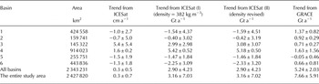
The overall mass change rate in the LAS and the trends at the basin level estimated from the 2004–2008 GRACE data are illustrated in the last column of Table 2. Basins 1, 2 and 3 show positive trends of 1.37 ± 0.82, 0.92 ± 0.29 and 0.71 ± 0.27 Gt a−1. The corresponding spatial pattern is clearly shown in Figure 12b. The other three basins (Basins 4, 5 and 6) have the estimated trends that are indistinguishable from zero. The trends estimated from the GRACE and ICESat data at the basin level are compared below. Note that the entire study area is larger than the sum of all the basin areas.
Table 2. Elevation and mass change rates and uncertainties (1σ) derived from 2004–2008 ICESat and GRACE data at the basin level (Fig. 1)
The observational errors are contained in the monthly GRACE gravity field solutions, which are further propagated to the estimated parameters, such as the trend, acceleration and others. Differences were calculated between the fitted curve in Figure 4 and the 57 monthly mass change solutions (black diamonds in Fig. 4) that were calculated based on the Stokes coefficients. The least-squares method that was used to estimate the parameters used these differences to calculate the variance of unit weight and variances of the estimated parameters through an error propagation law (Wahr and others, Reference Wahr, Swenson and Velicogna2006; Horwath and Dietrich, Reference Horwath and Dietrich2009; Ewert and others, Reference Ewert, Groh and Dietrich2012; Luo and others, Reference Luo, Li, Zhang and Wang2012). Consequently, the estimated linear trend of 7.66 Gt a−1 has an uncertainty of 5.91 Gt a−1. This uncertainty represents the effect of all categories of errors in the gravity field solutions.
The truncation of the spherical harmonic expansion and the filtering of the weight function resulted in so-called leakage errors. Leakage errors can be induced by changes in the storage of liquid water and snow on land beyond the ice sheet, ocean mass variability and ice loss from nearby ice caps. In Antarctica, this error can be as large as 20 Gt a−1 and tends to be greatest in West Antarctica, depending primarily on the weight function and filtering methods (Velicogna and Wahr, Reference Velicogna and Wahr2013). We used a hydrological model, the Global Land Data Assimilation System (GLDAS, version 1), to compute the leakage effect from water and snow on land beyond the ice sheet. The resulting values were then converted to spherical harmonic gravity coefficients and were removed from the GRACE Stokes coefficients (Velicogna and Wahr, Reference Velicogna and Wahr2013). The leakage error in the LAS estimate using GLDAS is 1.59 Gt a−1, and this value was used to correct the gravity field solutions.
The largest uncertainties result from the differences in the GIA corrections based on different models. We calculated corrections using three GIA models, namely the IJ05 R2, Paulson 2007 and W12a models. The resulting trends are 7.66 ± 5.91, 3.25 ± 6.88 and 30.38 ± 7.86 Gt a−1, respectively. The largest difference (between Paulson 2007 and W12a) is 27.13 Gt a−1. We used the result that applied corrections of the IJ05 R2 GIA model because its result is closest to the average of the results from the three GIA models investigated in this study. In addition, it has been used in many Antarctic mass-balance studies and fits well with Antarctic global GPS observations (Shepherd and others, Reference Shepherd2012).
Figure 5 presents the spatial distribution of GIA corrections from the IJ05 model in the forms of the mass correction (integrated at a resolution of 1° × 1°) and elevation correction (uplift). The spatial variation in the mass changes estimated from GRACE data is shown in Figure 12b.

Fig. 5. Spatial distribution of GIA corrections based on the IJ05 R2 model: (a) Mass correction (Gt a−1) integrated at a resolution of 1° × 1°. (b) Elevation correction (uplift) (mm a−1).
3. MASS CHANGE ESTIMATION FROM ICESAT DATA
3.1. ICESat data processing method
Mass changes can also be derived from ICESat observations of ice-sheet surface elevation change (SEC) (Zwally and others, Reference Zwally, Bindschadler, Brenner, Major and Marsh1989; Slobbe and others, Reference Slobbe, Lindenbergh and Ditmar2008). The amount of data and the spatial coverage are generally low when only crossover ICESat points are used. Therefore, we use repeated-track points to improve the spatial and temporal coverage. However, this method introduces uncertainties because the points are not located exactly in the same locations. Earlier methods used slope information in an external digital terrain model (DTM) to project ICESat points from one track to another and then compute elevation corrections. By doing so, errors in the DTM are propagated to the estimated elevation changes. An improved technique is to project the ICESat points of different tracks using the slope information from other ICESat points in the neighborhood instead of from an external DTM. This technique takes advantage of updated elevation/slope information of the same quality as the altimetric data (Schutz and others, Reference Schutz, Zwally, Shuman, Hancock and DiMarzio2005; Howat and others, Reference Howat, Smith, Joughin and Scambos2008; Gunter and others, Reference Gunter2009; Rémy and Parouty, Reference Rémy and Parouty2009; Moholdt and others, Reference Moholdt, Nuth, Hagen and Kohler2010; Liu and others, Reference Liu2012). Ewert and others (Reference Ewert, Groh and Dietrich2012) proposed a sophisticated method for mass-balance study in Greenland that involves estimating the elevation trends using repeated-track points in an area to fit a polynomial function that contains the elevation trend, the topography of the area and an annual term. The annual term was dropped because of the uncertainty that can be induced by only 2–3 campaigns of ICESat data a−1. This methodology was adopted, modified and implemented to perform the comparative study in LAS, East Antarctica.
The track separation was determined by examining the time flag. Repeated-track points were identified first by constraining the distance between the two tracks within 200 m. At a location on a track, we delineated a box measuring ~500 m × 500 m in the along- and across-track directions. All repeated-track points in the box were selected for the trend estimation. We employed a simplified spatial/temporal polynomial model based on Ewert and others (Reference Ewert, Groh and Dietrich2012) and Schenk and Csathó (Reference Schenk and Csathó2012) to characterize the ice surface topography and elevation trend, h′. For the ith repeated-track point (i = 1, 2,…, n) in the box with coordinates (x i , yi ), we have
 $${h_i} = h^{\prime}\,{t_i} + {a_{\rm o}} + {a_1}\,{x_i} + {a_2}\,{y_i},$$
where h i is the elevation; h′ is the trend and is assumed to be constant within the box; and t i is the time when the point was collected, which is referenced to the middle of the study period (1 June, 2006). The first term in Eqn (3) accounts for the temporal change. Because the box size of 500 m × 500 m is relatively small, the topography of the ice-sheet surface inside the box can be characterized as a plane with the first-order parameters a o, a 1 and a 2. Compared with the second-order model with ten unknown parameters in Ewert and others (Reference Ewert, Groh and Dietrich2012), this linear model with four parameters requires a relatively small number of repeated-track points (a minimum of four) in each box. Thus, it avoids a search for additional points in the along-track direction that may cause a biased estimate. This is particularly important for low-latitude areas where the tracks are increasingly separated (Fig. 6a) and the number of repeated-track points in an area is lower (see a later discussion). Once the parameters of h′, a o, a 1 and a 2 are estimated in a box, the process is repeated for the next box shifted 250 m from the previous location in the along-track direction. When this procedure is performed for all repeated tracks, a map of the elevation change trends in the study area based on the ICESat data can be produced.
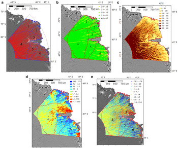
Fig. 6. (a) ICESat tracks in the LAS from February 2004 and October 2008, and major basins in the LAS (Zwally and others, Reference Zwally, Giovinetto, Beckley and Saba2012). (b) Number of years covered by all ICESat points in each box. (c) Number of boxes in each cell (30 km × 30 km) of a grid for computation of the trend in the study area and in each basin. (d) Elevation change trend (cm a−1) in each grid cell and (e) elevation change trend (cm a−1) in each box estimated from ICESat data for 2004–2008 after a GIA correction (IJ05 R2 model).
The ICESat/GLAS product (GLA12 R633) has 18 campaigns from January 2003 to October 2009 (2–4 campaigns a−1). To respond to a sensor problem (Schutz and others, Reference Schutz, Zwally, Shuman, Hancock and DiMarzio2005), the last campaign (Campaign 18) was not completed in accordance with its data acquisition plan. Furthermore, Campaign 17 yielded a significant number of empty data areas, based on our data quality examination. Thus, the data from these last two campaigns in 2009 were excluded from this study. To match the GRACE data of 2004–2010, we used 12 ICESat campaigns from 2004 to 2008 to perform a comparative study with the GRACE data for the LAS. The tracks of the ICESat dataset used in the study are illustrated in Figure 6a.
The ICESat points were selected to meet the following five geophysical requirements as proposed and used by Bamber and others (Reference Bamber, Gomez-Dans and Griggs2009a): (1) their attitude control in the metadata is classified as good, (2) only one waveform is detected, (3) the reflectivity of the surface exceeds 10%, (4) the gain is <200 and (5) the variance in the waveform from the Gaussian distribution is <0.03 V. Then, these selected points were projected from the TOPEX ellipsoid to the WGS84 ellipsoid and then from the WGS84 coordinate system to the Universal Polar Stereographic coordinate system.
Due to the error in the range determination from transmit-pulse reference-point selection during the 18 campaign periods, there are inadvertent range errors (called the Gaussian-centroid or ‘G-C’ offset) between ICESat campaign periods. These inter-campaign biases among the campaigns are reported to have a maximum impact of ± 10 cm a−1 on the elevation change estimates (Borsa and others, Reference Borsa, Moholdt, Fricker and Brunt2014). In this study, we corrected the inter-campaign biases using files provided by the National Snow and Ice Data Center (NSIDC, 2015). The elevation differences of all ICESat points of 2004–2008 in the study area before and after the corrections were calculated. Then the mean differences of each campaign were computed, ranging from ~−4 to 6 cm.
A GIA uplift correction calculated using the IJ05 R2 model compensates for the glacial isostatic rebound, which is of the order of −0.5 to 1.5 mm a−1 in the LAS region (Fig. 5b). This correction was applied to each ICESat point and corresponds to the GIA mass change correction applied in the GRACE data processing.
3.2. Elevation and mass changes in the LAS estimated from ICESat data
Overall, the ICESat data provide high-quality spatial and temporal coverage for estimating the elevation trend from 2004 to 2008. There are 808 517 repeated-track points and 736 092 boxes in the study area, with an average of ten repeated tracks and 29 repeated-track points in each box. The average temporal coverage of the points in each box is 4.7 a (Fig. 6b) and 99.94% of the boxes feature a temporal coverage that exceeds 2.5 a. The remaining 0.06% of the boxes (459 boxes) have a temporal coverage of 2–2.5 a and are in the low-latitude region, where the tracks gradually deviate from one another. Certain ICESat points were eliminated due to the effects of steep slopes in coastal areas. Thus, for the 1166 boxes in the coastal areas (<50 km from the coast) the average number of ICESat points in each box is 21. Overall, the spatial and temporal coverage is sufficient to determine the four parameters in Eqn (3).
Figure 6e shows the elevation change trend (cm a−1) in each box estimated from 2004–2008 ICESat data after the GIA correction. To calculate the overall trend in the entire study area and in each basin, we developed an intermediate-level grid with a cell size of 30 km by 30 km. Figure 6c illustrates the number of boxes in each grid cell. Within each cell (Fig. 6d), we calculated an average of all trend values of the boxes (Fig. 6e) in the cell. The 30 km cell size was determined to ensure more than five boxes in each cell for the average computation. Figure 6c indicates that in the high-latitude inland region, there are sufficient data to calculate the trend in each cell. In the low-latitude coastal areas, the quality of the average trend values may be compromised by the lower number of available original estimates from Eqn (3). We used only cells containing more than five boxes. Finally, we converted each cell's average trend value for elevation change to the corresponding mass change using a firn density of 382 kg m−3, which is an average of observations at 651 stakes along the CHINARE traverse (see description and discussion below).
The coastal region had a high snow accumulation rate during the study period, as evidenced by the snow stake observations along the CHINARE expedition traverse and the reports of Ding and others (Reference Ding2011, Reference Ding2013, Reference Ding2015). As shown in Figure 6e, a concentrated area of significant elevation changes is located on the west side of the Amery ice shelf, and several similar but smaller areas are spread along the coast east of the ice shelf. The upper interior region (Basin 4) receives less precipitation and consequently has lower positive elevation change rates. However, the basin has the largest area and even with low positive elevation change rates of each box in the basin; these cells collectively give Basin 4 the greatest mass change rate of 5.42 ± 0.52 Gt a−1 among the analyzed basins in the column of ‘Trend from ICESat (I)’ in Table 2. The change rates of other basins (Basins 1, 2, 3, 5 and 6) in the same column are not statistically distinguishable from zero. After the estimates of all basins are combined, the overall mass change rate in the LAS estimated from the 2004–2008 ICESat data is 3.16 ± 7.03 Gt a−1, i.e. not indistinguishable from zero.
Within each box used in the trend estimation, the least-squares process uses Eqn (3) and the repeated-track points in the box to estimate the four parameters as well as their uncertainties based on the error propagation law (Leick, Reference Leick2004; Ewert and others, Reference Ewert, Groh and Dietrich2012). The uncertainty (standard deviation (SD)) of the elevation of an ICESat repeated-track point, which is also the unit weight SD, σ o, is also estimated in each box. Its average from all basins is 8 cm with a range of 2–16 cm. Similarly, the uncertainty of the trend h′ in a box, σ h′, can also be calculated. Furthermore, we estimated the uncertainties in the 30 km × 30 km cells and then in the basins by using the scaled median absolute deviation (MAD) adopted from Ewert and others (Reference Ewert, Groh and Dietrich2012), which does not require a normal distribution. The detailed explanation of MAD is given in the Supplementary Materials. The estimated elevation trend uncertainties in the basins range from 0.2 to 5.4 cm a−1, which corresponds to an error in the mass change of 0.52–2.98 Gt a−1 (‘Trend from ICESat (I)’ in Table 2). At the basin level, the high-latitude inland region (Basin 4) has a higher density of ICESat points per estimation box (Fig. 6) and the slopes are generally low. Thus, the uncertainty in the elevation change rate for Basin 4 is the lowest (0.2 cm a−1). In contrast, Basins 2 and 3 are both in lower-latitude areas where the ICESat point density is lower. Furthermore, the steeper slopes in the coastal region of Basin 2 and the steep lateral slope of the Amery ice shelf in Basin 3 are disadvantageous for elevation change estimation. Hence, the uncertainties in the elevation change rates for these two basins are >5 cm a−1. Basins 1, 5 and 6 contain both coastal areas and the interior of the ice sheet, and their uncertainties in the trends are between the two extremes. Finally, the estimated trend for the entire study area is 3.16 Gt a−1, with an error of ± 7.03 Gt a−1 based on the uncertainty estimation.
4. COMPARISON OF THE ICESAT RESULT WITH SNOW STAKE MEASUREMENTS
4.1. Determination of firn density for elevation change to mass change conversion
The in situ observations are along the 1248 km CHINARE traverse route from Zhongshan station to Dome A (Fig. 1). The data available for this study include snow stake observations (surface firn density from 1999 to 2013 and heights from 2005 to 2008) on stakes at an interval of 10 km along the traverse. A dataset of firn depth/density measurements in a snow pit ~520 km from the coast is also available. Although the in situ observations do not represent the entire study area, they do serve limited ground-truth purposes for comparison with the result from the ICESat data. The processing and analysis results of the complete in situ observations from 1997 to 2013, including surface mass balance and snowdrift effects on snow deposition, have been published by Ding and others (Reference Ding2011, Reference Ding2013, Reference Ding2015).
The surface firn density of the upper 0.2 m was measured during the annual expeditions from 1999 to 2013. The density dataset made available to this study includes only one firn density at each of the 651 stakes along the traverse, which were aggregated from the observations from 1999 to 2013. The data were then smoothed using a 30 km moving-window-average filter to remove random noise (Fig. 7). Assuming there were no significant density changes in the study area during the observation period, we used the aggregated firn density data for our study of 2004–2008. The calculated firn density has an average of 382 kg m−3, with a SD of 30 kg m−3, and ranges from ~300 kg m−3 in the Dome A region to 453 kg m−3 close to the coast. Generally, the estimation of a long-term imbalance should use a density for the firn and ice column, such as 900 kg m−3 for the ERS data of 1992–2001 (Zwally and others, Reference Zwally2005). The present study has a relatively short period of 2004–2008 and we applied this average of the surface firn density measurements for conversion of the ICESat elevation trend to the mass trends in the column of ‘Trend from ICESat (I)’ in Table 2.

Fig. 7. Aggregated firn density measurements at snow stakes from 1999–2013 along the CHINARE traverse and smoothed using a 30 km moving-window-average filter. The horizontal axis represents the distance to the coast (km) and the vertical axis shows the firn density (kg m−3).
An experiment was also performed to adjust the firn densities of the basins using the in situ density measurements along the CHINARE traverse to deal with spatial variation. First, a linear regression was carried out between the distance to the coast (x) and the density measurements (y) in Figure 7. A linear function, y = −0.005x + 400.1 is estimated (red line, Fig. 7), with a correlation coefficient of r = 0.6. The density profile shows a decreasing trend from the coast to the high interior.
Second, a centroid for each basin was determined using a GIS (ESRI, 2014) (Fig. 8). In order to facilitate the computation of the distances from the centroids to the coast, a generalized coast line (green; Fig. 8) was produced by the GIS system based on the detailed MODIS Mosaic of Antarctica (MOA) grounding line (Haran and others, Reference Haran, Bohlander, Scambos, Painter and Fahnestock2014). The calculated distances to the coast for all basins and for the study area are listed in Table 3. Based on the distances the firn density for each basin is then computed using the density/distance regression function and is illustrated in Table 3. Finally, the mass change rates of the basins were recalculated using the new density values and presented in the column, ‘Trend from ICESat (II)’ in Table 2.

Fig. 8. Centroids of basin boundaries (red dots) and the generalized coast line (green) which were used to adjust the density of each basin.
Table 3. Firn density recalculated for each basin using an aggregated function from the in situ measurements along the CHINARE traverse

It is observed that the coastal basins (Basins 1, 2, 3 and 6) have their distances to the coast shorter than the half-length of the traverse. Their calculated firn densities are also greater than the average density of 382 kg m−3 (last two columns in Table 3). Correspondingly the magnitude of their adjusted mass trends in column, ‘Trend from ICESat (II)’ increased by 3–6% compared with these in column, ‘Trend from ICESat (I)’ in Table 2. In contrast Basins 4 and 5 are farther away from the coast and thus obtained reduced densities in Table 3. Similarly the magnitude of their adjusted mass trends in the column, ‘Trend from ICESat (II)’ decreased by 5% for Basin 4 and 1% for Basin 5. The overall densities and trends of all basins and the study area remained unchanged. Although the trends of the individual basins were adjusted by <6%, the adjustment was performed based on their proximities to the coast and the in situ density measurements. The adjusted trends in Table 2 were adopted.
4.2. Comparison of ICESat result with snow stake accumulation measurements
Surface snow accumulation rate from the snow stake observations along the CHINARE traverse is illustrated as red dots in Figure 9. The smoothed accumulation rate (light blue curve) was produced by filtering with a 30 km moving-window average, which can be considered as the surface height change (SHC) rate. The mean difference between the raw stake data and the smoothed curve is −0.05 cm a−1 with a SD of 11 cm a−1. A detailed surface mass-balance analysis with respect to local and regional terrain using snow stake observations from a longer period is provided by Ding and others (Reference Ding2011, Reference Ding2015). The rate of SEC from ICESat data after the GIA correction was extracted from the 30 km resolution ICESat 2004–2008 trend map (Fig. 6d) and is represented by the dark curve line in Figure 9. In the inland section of relatively flat, high-elevation terrain located 220–1248 km from the coast, the SHC rate has average, 15 cm a−1 with SD, 6 cm a−1 and the SEC rate from the ICESat data has average, 1 cm a−1 with SD, 2 cm a−1. Thus, their difference is 14 cm a−1. In the coastal section, i.e. from the coast (Zhongshan Station) to 220 km inland, where the topography changes rapidly from near sea level to an elevation of ~2100 m, the SHC rate is highest with average, 37 cm a−1 and SD, 7 cm a−1. The SEC rate from the ICESat data has a significantly contrasting trend, i.e. an average, −6 cm a−1 with SD, 0.85 cm a−1. This results in a difference of 43 cm a−1 in the coastal section and should be investigated further.

Fig. 9. Snow accumulation rate from 2005 to 2008 snow stake observations (red dots), smoothed snow accumulation rate after filtering with a 30 km moving-window average (light blue), SEC rate from 2004 to 2008 ICESat data after GIA correction (dark blue), and elevation profile along the CHINARE traverse from Zhang and others (Reference Zhang, Dongchen, Wang, Li, Jin and Zhou2008).
In general, a relationship exists between the measured SEC and the local mass-balance components (Csatho and others, Reference Csatho2014; Li and Zwally, Reference Li and Zwally2011):
 $${\rm SEC} + {\rm GIA\_Corr} = {\rm SHC} + {\rm Singk\_Corr} + {\rm DVEC}{\rm.} $$
The GIA correction (uplift), GIA_Corr (mm a−1), is shown in Figure 5b. The SHC represents the surface mass balance and is computed from the stake observations, which contain the effects of the summed changes that have occurred above the stake bottom, such as precipitation, sublimation, meltwater, runoff and others. Singk_Corr corrects for the sinkage of the stakes due to snow compaction. Finally, DVEC is the vertical elevation change below the stake bottom that should represent the dynamic thickness change. Equation (4) can be rewritten as
 $${\rm SHC} - {\rm SEC} - {\rm GIA\_Corr} = - {\rm Singk\_Corr} - {\rm DVEC}{\rm.} $$
The vertical surface difference after the GIA correction (SHC − SEC − GIA_Corr) can be calculated from the processed snow stakes and ICESat results in Figure 9 and is illustrated in Figure 10, where the black dots represent the differences between the snow stakes and the ICESat results at the stake locations. The red curve is the 30 km moving-window average of the differences.

Fig. 10. Differences between the 2005–2008 snow stakes and 2004–2008 ICESat results at the stake locations (black dots), the 30 km moving-window average of the differences (red), and the ice flow speeds (blue dots, green triangles and yellow squares) along the CHINARE traverse.
The comparison between the SHC and SEC rates only makes sense if the background sinking of the stakes due to densification below the stake base and vertical flow of the ice, which are expressed on the right-hand side of Eqn (5), are taken into account (Dibb and Fahnestock, Reference Dibb and Fahnestock2004). An effort was made to compute the sinkage corrections according to Takahashi and Kameda (Reference Takahashi and Kameda2007) and Eisen and others (Reference Eisen2008) using the available depth/density data at the only snow pit 520 km from the coast. However, this effort resulted in unreasonable corrections in the Dome A region. Thus, the sinkage correction was not performed in this study. Ding and others (Reference Ding2015) indicated that the uncertainty of surface mass balance caused by densification in this region is ~−1.9% at 296 km from the coast (coastal section), −3.5% at 800 km (inland section) from the coast and 0% at Dome A for a 5 a snow layer. Given the SHC averages and the above uncertainty values, the estimated uncertainty of the average SHC rates may be −0.6 cm a−1 in the coastal section, −0.5 cm a−1 in the inland section and zero at Dome A. Therefore, these values should not play a major role in the differences between the rates derived from the stakes and the ICESat data, which are on average 31 cm a−1 in the coastal section and 12 cm a−1 in the inland section.
We do not have direct information on the dynamic thickness changes along the traverse, i.e. DVEC in Eqn (5). However, two sources of the ice flow speed are available. At each stake location, the horizontal ice flow speed along the traverse (blue dots; Fig. 10) was extracted from an ice flow-speed map of Antarctica from 2007 to 2009, which was estimated from satellite SAR and InSAR observations (Rignot and others, Reference Rignot, Mouginot and Scheuchl2011b). The zero speed dots that are circled in the coastal section appear to be inconsistent with the rest of the entire speed curve based on a visual inspection of the speed map and optical satellite images. A set of GPS points along the same traverse is also available: 19 CHINARE points were measured in 1997–2004 (green triangles; Fig. 10) and 13 ANARE points were measured in 1993–1994 (yellow squares; Fig. 10) (Manson and others, Reference Manson, Coleman, Morgan and King2000; Zhang and others, Reference Zhang, Dongchen, Wang, Li, Jin and Zhou2008). The ice flow-speed values of the GPS points and the speed map agree in the inland section with an average difference, 0.4 m a−1, SD of 1.2 m a−1. A greater difference exists in the coastal section, with average difference, 6.4 m a−1, SD 26.7 m a−1. The complete profile of the ice flow speed consists of the speed data from the InSAR ice flow-speed map and the GPS speed observations of the CHINARE and ANARE expeditions. The combined ice flow-speed profile is also filtered with a 30 km moving-average filter.
In principle, dynamic thickening/thinning of the ice sheet is not directly related to the horizontal ice velocity, but to the acceleration, which is not available in this study. There may be a correlation between horizontal ice velocities and accelerations, and thus between horizontal ice velocities and dynamic thinning. Such a correlation may imply causation. The ice flow-speed profile (horizontal) and the curve of the differences between the stake and ICESat observations in Figure 10 are correlated (r = 0.65). In the coastal section, the location around the highest speeds corresponds with an upstream area of a tributary ice flow into the Amery ice shelf, as shown on the ice flow-speed map (Rignot and others, Reference Rignot, Mouginot and Scheuchl2011b). This relatively high level of correlation indicates that dynamic thinning may explain the significant difference between the high accumulation measurements from the snow stakes and the decreased trend from the ICESat data in the coastal section.
Although there is no in situ measurement coverage of accumulation in the entire coastal section of the study area, a correlation between the ICESat trend and ice flow speed was performed. First, a coastal zone of 250 km from the grounding line/coastline was defined, which is in the grounded portion of the ice sheet in the study area. Then the ICESat trend of 2004–2008 in the 30 km × 30 km grid (Fig. 6d) was clipped using the 250 km coastal zone (Fig. 11a). The ice flow speed in the coastal zone was resampled at 30 km × 30 km cells from the ice speed map in Rignot and others (Reference Rignot, Mouginot and Scheuchl2011b). A correlation coefficient between the ICESat trend and ice flow speed, ${\rho _{{\rm Spee}{{\rm d}_i}}}$
, was calculated using the ice flow-speed cells with values greater than ‘Speed
i
’ and the corresponding ICESat trend cells. Figure 11b plots the correlation coefficients for ice flow speed from 0 to 500 m a−1. There is no significant correlation until Speed
i
= 222 m a−1; after that the correlation coefficient is >0.65 and reached 1 at about 340 m a−1 (Fig. 11b). We can observe that in Figure 11a the negative trend cells (light to dark blue dots) appear mostly near and along the ice flow lines (thin black) where the ice flow speed is high, except for some areas in Basin 3. This spatial correlation pattern may suggest that the dynamic ice thickness changes caused by the ice flows may have exceed the high snow accumulation rates in these places of the coastal section.
${\rho _{{\rm Spee}{{\rm d}_i}}}$
, was calculated using the ice flow-speed cells with values greater than ‘Speed
i
’ and the corresponding ICESat trend cells. Figure 11b plots the correlation coefficients for ice flow speed from 0 to 500 m a−1. There is no significant correlation until Speed
i
= 222 m a−1; after that the correlation coefficient is >0.65 and reached 1 at about 340 m a−1 (Fig. 11b). We can observe that in Figure 11a the negative trend cells (light to dark blue dots) appear mostly near and along the ice flow lines (thin black) where the ice flow speed is high, except for some areas in Basin 3. This spatial correlation pattern may suggest that the dynamic ice thickness changes caused by the ice flows may have exceed the high snow accumulation rates in these places of the coastal section.
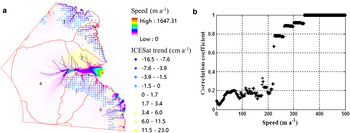
Fig. 11. (a) Three layers of information prepared for correlation analysis: Elevation trend of 2004–2008 in a 30 km × 30 km grid derived from the ICESat data and clipped inside a 250 km coastal zone, ice flow speed by Rignot and others (Reference Rignot, Mouginot and Scheuchl2011b), and generalized ice flow lines (black) from Liu and others (Reference Liu2015). (b) Correlation between the ice speed and ICESat trend estimates.
5. RECONCILED GRACE/ICESAT ESTIMATE AND SPATIAL ANALYSIS
The GIA effect was corrected in both GRACE and ICESat results. The SEC derived from the ICESat data reflect the surface mass balance (SHC), firn compaction (Singk_Corr) and ice dynamic changes (DVEC) in Eqn (4) when it is applied to the entire LAS study area. The rate of firn compaction is associated with elevation changes, but it does not involve changes in mass (Zwally and Li, Reference Zwally and Li2002). As shown in the previous section, the uncertainty caused by firn compaction in this study is not significant (Ding and others, Reference Ding2015). If it is assumed that the vertical ice velocity (ice flow) is in balance with the long-term average accumulation rate, the elevation changes can be attributed to accumulation anomalies over the observed period. Thus, although elevation change rates are significant in some local areas (Figs 6e, 11a), the overall ICESat trend of 0.3 ± 0.7 cm a−1 from 2004 to 2008 in the LAS region (Table 2) is statistically indistinguishable from zero.
The mass change estimated using the GRACE observations represents the overall change, including the surface mass change, changes caused by subglacier activities and mass changes beneath the ice sheet. The mass change rate of 7.66 ± 5.91 Gt a−1 in the LAS from the GRACE data (Table 2) is not significantly different from the rate of 3.16 ± 7.03 Gt a−1 from the ICESat data, given their uncertainties (1σ). We combined the two results from the GRACE and ICESat data to achieve a reconciled trend in the LAS from 2004 to 2008 by using the arithmetic mean, 5.41 Gt yr−1 and the uncertainty of the arithmetic mean (1σ; S3 in the Supplementary Material), 4.59 Gt a−1.
With regard to the recent mass balance in the LAS summarized in Table 1, the estimates of 1992–2003 from the ERS data by Zwally and others (Reference Zwally2005) and Wingham and others (Reference Wingham, Shepherd, Muir and Marshall2006b) are contradictive and we cannot reach a conclusion based on the discussion in the introduction section. The same applies to the opposite estimates of 2000 using the input/output method of Rignot and others (Reference Rignot2008) and Yu and others (Reference Yu, Liu, Jezek, Warner and Wen2010). However, both LAS-specific research efforts using in situ measurements by Ren and others (Reference Ren, Allison, Xiao and Qin2002) (though without an uncertainty specification) and Yu and others (Reference Yu, Liu, Jezek, Warner and Wen2010) resulted in positive estimates. Furthermore, the results of both earlier GRACE studies showed positive trends, 36 ± 11 Gt a−1 from 2002 to 2010 by King and others (Reference King2012) and 35 ± 8 Gt a−1 from 2003 to 2012 by Sasgen and others (Reference Sasgen2013). In comparison with the estimate of 7.66 ± 5.91 Gt a−1 of 2004–2008 from the GRACE data in this study, the difference in the magnitude may be attributed mainly to the different integration lengths (8–10 a vs 4.75 a). The long-term trend is advantageous in eliminating or reducing the effect of multiyear annual changes and short-term anomalies. On the other hand, the GRACE estimate of 2004–2008 is sufficient to capture a shorter term trend of mass changes in the LAS, which agrees with the estimate of the same period from the ICESat data and in situ CHINARE measurements. The reconciled trend in the LAS of 2004–2008 from both GRACE and ICESat estimates, 5.41 ± 4.59 Gt a−1, is also in line with another short-term estimate of 2010–2013 from the CryoSat-2 data, 2 ± 18 Gt a−1, by McMillan and others (Reference McMillan2014).
Overall, we suggest a balanced to slightly positive mass balance in the LAS from 2004 to 2008, given the level of the uncertainty. The LAS may have a positive mass balance since 1994 (Ren and others, Reference Ren, Allison, Xiao and Qin2002); a definite positive trend has existed at least since 2002 (King and others, Reference King2012; Sasgen and others, Reference Sasgen2013); and this positive change rate may have slowed in recent years (this study; McMillan and others, Reference McMillan2014).
To compare the spatial variations, Figure 12 presents the mass change rates of ICESat and GRACE in a grid with a cell size of 30 km × 30 km where the ICESat result was converted from the aggregated elevation trend map (Fig. 6d), whereas the GRACE result was interpolated from a grid with a much larger cell size of 1° × 1°. The ICESat trend map shows a higher level of spatial detail. The GRACE trend map appears to be a highly spatially aliased version of the ICESat trends. The relatively low level of positive rates across the vast high-latitude inland area (Basin 4) is consistently shown in both the ICESat and GRACE results. Correspondingly, Basin 4 has the highest trends from both the ICESat and GRACE data (Table 2). The negative trend of Basin 5 appears also consistently in both maps.

Fig. 12. Trend maps for the LAS from 2004 to 2008 (Gt a−1; resolution 30 km × 30 km): (a) Mass change rate from ICESat data and (b) corresponding rate from GRACE data.
The high change rates in both datasets occur in the coastal areas (Fig. 12). However, these rates are spread broadly across more basins in the GRACE result than in the ICESat result. For example, the red area of the high ICESat positive trend in Basin 6 (Fig. 12a) was detected by relatively densely populated ICESat points (Fig. 6). In the GRACE map (Fig. 12b), the corresponding high positive rates are centered at about the same location, but across a larger region (~300 km × 440 km). Although the original GRACE points were integrated at a resolution of 1° × 1°, which was output at a higher spatial resolution in this high latitude region (Fig. S2; Supplementary Material), at a global level GRACE can resolve features of ~400 km to 600 km (Tapley and others, Reference Tapley, Bettadpur, Ries, Thompson and Watkins2004b). Thus, the area in the GRACE map (~300 km × 440 km) would just be resolvable. The reddish color shades (high positive trend values) of the 30 km × 30 km cells in the expanded area are mainly attributed to the resolution of the GRACE solution and the effect of the interpolation. Furthermore, the high ICESat positive trends in Basin 3 occupy a concentrated area (Fig. 12a). However, its center is shifted by ~400 km to Basin 2 in the GRACE map and the high positive trends spread across a much larger area. The expansion of the area can also be mainly explained by the low resolution of the GRACE solution and the interpolation effect. But the shift of the areal center may indicate that the data are affected by so-called ‘internal leakage errors’ (King and others, Reference King2012; Memin and others, Reference Memin, Flament, Rémy and Llubes2014), which account for effects of the leakage from neighboring basins. A quantitative confirmation and analysis of this effect are beyond the scope of this study and will be our future research. Overall these cross-basin spatial variations may be caused by the resolution difference between the ICESat and GRACE data, the interpolation effect and the internal leakage errors, among others. Combined with the uncertainty in the firn density, these effects further caused the disagreement between the GRACE and ICESat results in Basins 1, 2, 3 and 6 (Table 2).
6. CONCLUSIONS AND DISCUSSIONS
This paper presents the results of a comprehensive study of the regional mass changes from 2004 to 2008 in the LAS, Antarctica, using GRACE, ICESat and in situ CHINARE data. A survey and analysis of the recent research results in the LAS was performed. The present results were achieved by using both satellite remote sensing data and regional in situ measurements, and contribute to the understanding of the long-term mass balance and quantification of the trend in the recent years in the study area. The estimation of the ICESat mass change rates benefitted from the density measurements along the CHINARE traverse and a spatial density adjustment method for reducing the effect of spatial density variations. The CHINARE surface accumulation measurements and surface ice flow-speed data were analyzed jointly with the ICESat elevation changes to investigate the regional mass-balance details. Finally, the mass change rate of 2004–2008 in the LAS was determined by a reconciled GRACE/ICESat estimation. The following are the discussions and conclusions of this study:
-
(1) Uncertainties in the firn density have been one of the major error sources for mass change estimation from altimetry data. The surface firn density measurements along the CHINARE traverse showed a variation from ~300 kg m−3 in the Dome A region to 453 kg m−3 at the coast. The average of 382 kg m−3 was used for the ICESat mass trend estimate during the period of 2004–2008, which was further improved by a spatial density adjustment method for reducing the effect of spatial density variations in the entire study area. The achieved regional ICESat mass trend, 3.16 ± 7.03 Gt a−1, agreed with that derived from the overlapping GRACE data, 7.66 ± 5.91 Gt a−1, given their uncertainties.
-
(2) Along the CHINARE traverse the ICESat elevation change rate was closer to the snow stake surface change rate with an average difference of 14 cm a−1 in the inland section (220–1248 km from the coast). The same difference rose to 43 cm a−1 in the coastal section (0–220 km from the coast). A correlation coefficient of 0.65 is achieved between the ice flow speed and the difference between the snow stake and ICESat results along the traverse. A further analysis investigated the correlation between the ICESat trend and ice flow speed in the coastal region of the entire LAS. The correlation coefficient is >0.65 if the flow speed >222 m a−1 and 1 above ~340 m a−1. The above result suggests that during the study period the dynamic ice flow discharge surpassed the snow accumulation in many high flow-speed glacier areas along the coast.
-
(3) At the basin level, both the ICESat and GRACE results agree in places where significant changes exist and the areas are greater than the feature size that the GRACE solutions can resolve. For example, the vast high-elevation inland region receives less precipitation and, thus, has a low level of positive elevation change rate in each cell. Due to its large area, Basin 4 exhibits the greatest mass change rates from both GRACE and ICESat data among the basins. On the other hand, the GRACE trend map appears to be a highly spatially aliased version of the ICESat trends. The largest positive mass changes occur in the coastal region. But there are differences in their areal sizes and a shift of centers. The difference in areal sizes can be attributed to the different resolutions and effect of interpolation; the shift of the areal centers may be caused by so called ‘internal leakage errors’, which needs to be further researched. These cross-basin discrepancies in spatial variations further caused the basin level disagreements between the GRACE and ICESat estimates in Basins 1, 2, 3 and 6.
-
(4) Overall, the reconciled trend in the LAS of 2004–2008 from both GRACE and ICESat estimates is 5.41 ± 4.59 Gt a−1. With regard to the recent mass balance in the LAS, a positive mass balance may have occurred at a rate of 17 Gt a−1 (no uncertainty given) during the period of 1994–1999 based on an estimate using both CHINARE and ANARE in situ measurements (Ren and others, Reference Ren, Allison, Xiao and Qin2002). The positive trends of 36 ± 11 Gt a−1 from 2002 to 2010 and 35 ± 8 Gt a−1 from 2003 to 2012 in the LAS were derived from the results by King and others (Reference King2012) and Sasgen and others (Reference Sasgen2013) respectively; these estimates showed a long-term trend after removing the effect of multiyear annual changes and short-term anomalies. In this study, the reconciled trend of 5.41 ± 4.59 Gt a−1 from 2004 to 2008 was estimated using the GRACE, ICESat and CHINARE in situ data; this estimate indicated a shorter-term trend of balanced to slightly positive mass changes in the LAS. This positive mass trend in the LAS may have slowed down recently based on another shorter-term estimate of 2 ± 18 Gt a−1 from 2010 to 2013 that was derived from the CryoSat-2 result by McMillan and others (Reference McMillan2014).
SUPPLEMENTARY MATERIAL
The supplementary material for this article can be found at http://dx.doi.org/10.1017/jog.2016.76.
ACKNOWLEDGEMENTS
Constructive comments and suggestions by editors and two reviewers are greatly appreciated. Data from National Snow and Ice Data Center (NSIDC), University of Colorado, Center for Space Research (CSR), University of Texas at Austin, CHINARE and ANARE programs, and Polar Research Institute of China are also greatly appreciated. The work described in the paper was substantially supported by the National Basic Research Program of China – 973 Program (Project Nos 2012CB957701, 2012CB957702), the National Natural Science Foundation of China (Project Nos 41201426, 41325005, 41571407), the Shanghai Rising-Star Program (Project No. 15QA1403700) and the Fundamental Research Funds for the Central Universities.


 Open access