


1 Introduction
Cross-field (across the background magnetic field) transport of charged particles is gaining attention in low temperature plasmas (Curreli & Chen Reference Curreli and Chen2014) in addition to its strong relevance in magnetically confined high temperature plasmas. This is due to, for instance, its relevance to linear plasma generators (Owen et al. Reference Owen, Caneses, Canik, Lore, Corr, Blackwell, Bonnin and Rapp2017), industry applications using magnetrons or helicons (Curreli & Chen Reference Curreli and Chen2014) and Langmuir probe diagnostics of magnetized plasmas (Popov et al. Reference Popov, Dimitrova, Ivanova, Kovačič, Gyergyek, Dejarnac, Stöckel, Pedrosa, López-Bruna and Hidalgo2016). We investigate such cross-field transport in a curved magnetic field geometry including a magnetic X-point. The two-wire model (TWM) is the magnetic configuration generated by the axially flowing two parallel currents which form a magnetic X-point at the centre. The TWM is of research interest as it resembles the magnetic configurations of single-null diverted tokamaks and those of the magnetic reconnections (Auerbach & Boozer Reference Auerbach and Boozer1980). Understanding plasma transport in the TWM configuration, especially in the vicinity of the X-point, can help us to comprehend how plasmas are lost to the divertors as well as their spatial profiles in the scrape-off-layer region in tokamaks, which are active research topics for controlling the heat and particle fluxes associated with fusion-grade hot plasmas (Pitcher & Stangeby Reference Pitcher and Stangeby1997; ITER Divertor Physics Expert Group on Divertor and ITER Physics Expert Group on Divertor Modelling and Database and ITER Physics Basis 1999; Loarte et al. Reference Loarte2007; Soukhanovskii Reference Soukhanovskii2017; Innocente et al. Reference Innocente, Ambrosino, Brezinsek, Calabrò, Castaldo, Crisanti, Dose, Neu and Roccella2022). Furthermore, a collisionless transport phenomenon with the finite Larmor-radius (FLR) effect is deemed significant in a magnetic island with the gyrokinetic approach (Choi & Hahm Reference Choi and Hahm2022; Choi Reference Choi2023).
Numerous studies about the TWM have been performed in the past. Reiman (Reference Reiman1996) identified a set of singular surfaces in the TWM open field line region, which plays a role of rational surfaces and separatrices in toroidal plasmas. Ali, Punjabi & Boozer (Reference Ali, Punjabi and Boozer2009) studied the magnetic field structure in the vicinity of the separatrix of the TWM. Auerbach & Boozer (Reference Auerbach and Boozer1980) studied classical diffusion in the TWM. They superposed axial (toroidal) magnetic fields, making the Larmor radii small enough even at the X-point such that the FLR effects could be neglected.
We are, on the other hand, interested in properties of plasmas in the basic TWM, i.e. no superposed axial magnetic fields, as it intensifies the effects of spatially varying magnetic fields and the FLR on plasma behaviours near the X-point region where the total field strength approaches zero. Only two circular fields produced by the two current carrying wires are combined to make a figure-eight shaped two-dimensional TWM field in this work. Recently, a low temperature plasma device was developed to experimentally investigate plasmas in such fields (Lim et al. Reference Lim, You, Lee, Ahn, Moon, Kim, Woo, Lho, Choe and Ghim2020), where interesting plasma profiles were reported around the X-point.
Owing to its large spatial gradient of the magnetic field and the FLR near the X-point, the study of plasma properties in the TWM configuration with kinetic theory or fluid models can be expensive; thus, we numerically investigate a single particle motion which allows us to understand plasma transport in the collisionless limit and to gain a physical intuition of such plasmas. In fact, there have been several related studies with single particle motions. Sonnerup (Reference Sonnerup1971) studied adiabatic particle orbits in a magnetic null sheet and conserved quantities of interest. Kim & Cary (Reference Kim and Cary1983) analysed charged particle motions near a linear magnetic null. Numata & Yoshida (Reference Numata and Yoshida2002, Reference Numata and Yoshida2003) studied collisionless resistivity in the magnetic null region by analysing chaotic orbits of particles. Chirikov (Reference Chirikov1960) reported resonant effects between the gyro-frequency and the bounce frequency in a magnetic trap that can cause variations of the magnetic moment and subsequent particle loss from a magnetic trap. Büchner & Zelenyi (Reference Büchner and Zelenyi1989) investigated non-adiabatic trapped particle motions in magnetic field reversals and showed how the curvature of the fields determines different types of particle trajectories.
The purpose of this paper is to numerically investigate collisionless transport of charged particles near the X-point in the TWM configuration based on single particle motion. In this study, the term collisionless specifically means single particle motion without considering the influence of electric and magnetic fields induced by other charged particles. Gyrating particles are guided along the corresponding base field line (invariant), which is determined by the axial canonical momentum, one of the two conserved quantities in the TWM. The other conserved quantity is the total kinetic energy. As the particles travel along the base field line, they can enter a region where a spatial gradient of the field is large, i.e. near the X-point, and it causes the first adiabatic invariant, the magnetic moment $\mu =W_\perp /B$ , to change (Stephens, Brzozowski & Jenko Reference Stephens, Brzozowski and Jenko2017), which, then, can lead to collisionless transport. Here, $W_\perp$
 and $B$
 are the perpendicular kinetic energy and the magnetic field magnitude, respectively. Specifically, when the magnetic moment becomes large, resulting in a large Larmor radius, particles probabilistically cross the separatrix to migrate to the opposite side of the TWM configuration.
We find that a seemingly random shift of the magnetic moment near the X-point is, in fact, statistically well behaved and with a property that is completely determined by the two conserved quantities, i.e. the total kinetic energy and the axial canonical momentum or the base field line value. We also find that there exists a threshold energy allowing only particles with a higher energy to cross the separatrix and migrate, where the threshold energy is determined by the base field line value. Note that a migrating particle experiences the reversal of the magnetic field direction, resulting in a betatron orbit, similar to orbits found near null regions of field-reversed-configuration plasmas (Welch et al. Reference Welch, Cohen, Genoni and Glasser2010). The crossing time is found to be exponentially distributed and its average, which we denote as the migration confinement time, is shorter for particles with a base field line closer to the separatrix and a higher energy. The migration confinement time is heuristically formulated with the simulation results so that time scales of the collisionless transport can be readily estimated.
The outline of this paper is as follows. We first introduce the formula, geometry and characteristics of the TWM in detail in § 2. Then, with the equation of motion, invariants that govern the particle motion are explained in § 3 as well as the simulation method and its conditions. With an example, two phenomena of interests, i.e. magnetic moment shift and the migration, are also discussed in this section. In § 4, the statistical property of magnetic moment shift is analysed. In § 5, the migration phenomenon is discussed. The necessary condition for the migration to occur is derived, and the migration confinement times are empirically formulated. Then, the summary and conclusion are given in § 6.
2 Two-wire model
To investigate the single charged particle motion, we first introduce the TWM configuration. The TWM is the one of the simplest analytic geometries that contains the magnetic X-point. In the TWM, we place two axial current carrying wires at the positions of $x=0$ and $y=\pm \ell$
 . The current $I$
 is applied to both wires. Then, the field of the TWM can be expressed as

where $A_0 = I\mu _0/2{\rm \pi}$ is the system magnetic flux, $\mu _0$
 is the vacuum permeability, $y_\pm = y\pm \ell$
 , $r^2 = x^2+y^2$
 and $r_\pm ^2 = x^2+y_\pm ^2$
 .
.
Normalization is performed to make all quantities dimensionless, so that the results of this investigation can be applied to systems with any scale. The normalized TWM field can be written as
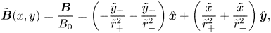
where $B_0 = A_0/\ell$ is the system field magnitude, $\tilde {x} = x/\ell$
 , $\tilde {y} = y/\ell$
 , $\tilde {y}_\pm = y/\ell \pm 1$
 , $\tilde {r}^2 = \tilde {x}^2 + \tilde {y}^2$
 and $\tilde {r}_\pm ^2 = \tilde {x}^2 + \tilde {y}_\pm ^2$
 . In this work, the subscript ‘$0$
 ’ is used to describe system characteristic quantities, whereas the tilde hat, i.e. ‘$\tilde {x}$
 ’, is used to denote normalized dimensionless quantities.
Realizing that we can express the magnetic field as ${\boldsymbol B}={\hat {\boldsymbol z}}\times \boldsymbol {\nabla } \psi$ due to there being no axial magnetic fields, a field line (flux surface) of the TWM can be formulated as


where a constant $s$ or $\psi$
 draws a field line. Notice that (2.4) is the equation for the Cassini oval (see figure 1). The separatrix is at $s=1$
 , or equivalently $\psi =0$
 .
.
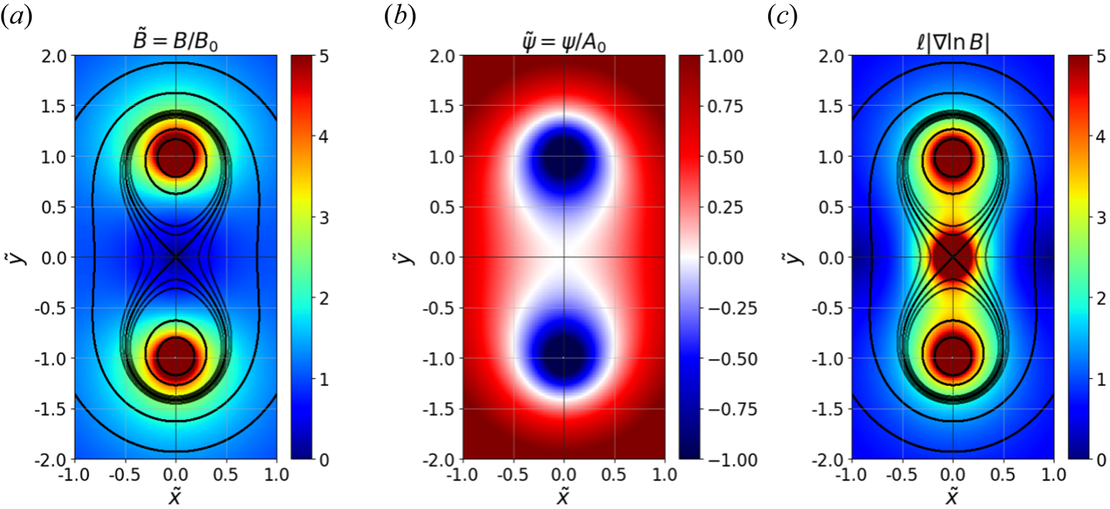
Figure 1. Generated magnetic field with the TWM where the single particle motion is investigated in this work. (a) Normalized magnitudes of the magnetic field $\tilde {B}$ with overlaid $\tilde {\psi }$
 drawn in black lines from $-1$
 to $1$
 ($-1, -0.5, -0.1, -0.05, 0, 0.05, 0.1, 0.5, 1$
 ). The field lines inside the figure-eight shaped separatrix have negative $\tilde {\psi }$
 . (b) Normalized field line values $\tilde {\psi }$
 . It is zero, i.e. white colour, at the separatrix. (c) Normalized gradient scale lengths of the magnetic field $\ell |\boldsymbol {\nabla } \ln B|$
 with the overlaid $\tilde {\psi }$
 drawn in black lines whose values are the same as in (a).
Finally, the normalized magnitude and gradient scale length of the magnetic field in the TWM configuration are, respectively,


Figure 1(a) shows normalized magnitudes of the magnetic field, which becomes infinitely strong at the wires and becomes null at the X-point. Figure 1(b) shows the corresponding normalized field line values $\tilde {\psi }$ , which are negative (positive) inside (outside) the separatrix where the field line value is zero. Figure 1(c) shows normalized gradient scale lengths of the magnetic field, and the gradient becomes infinitely large at the X-point. Since the magnetic field magnitude changes fast in space around the X-point, the magnetic moment $\mu$
 cannot be conserved properly (Stephens et al. Reference Stephens, Brzozowski and Jenko2017). This phenomenon and its consequences are discussed in detail with numerical results in § 4 and § 5.
3 Single particle motion
Single charged particle motion in the TWM configuration is studied numerically at the collisionless limit. At this limit, interactions among particles through induced electric and magnetic fields are neglected. Therefore, only the externally applied TWM field governs the motion of the particles, and the equation of motion is given as

where $\omega _{c0}=qB_0/m$ is the system cyclotron frequency, $q$
 and $m$
 are, respectively, the charge and mass of the particle of interest. In addition, $\tau _0=2{\rm \pi} / |\omega _{c0}|$
 is the system gyro-period, that normalizes temporal quantities in this study; $v_0=qA_0/m=\ell \omega _{c0}$
 and $W_0=mv_0^2/2$
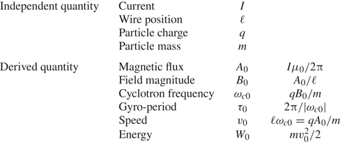
 are the system speed and energy, which normalize speed and energy quantities, respectively. As there are various normalizing quantities in this work, they are summarized in table 1.
Table 1. System quantities used to normalize various physical parameters in the TWM.
3.1 Constants of motion: the total kinetic energy and the base field line value
There are two constants of motion in this system: the total kinetic energy $W_\text {total}$ , and the base field line value $\psi _\text {base}$
 . Since the magnetic field alone does no work, the total energy, $W_\text {total}=mv^2/2$
 , is conserved. The Lagrangian $\mathcal {L}$
 and the axial canonical momentum $p_{z,\text {can}}$
 of the system are

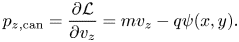
By the Euler–Lagrange equation, i.e. ${\rm d} p_{z,\text {can}}/{\rm d} t=\partial \mathcal {L}/\partial z=0$ , we see that $p_{z,\text {can}}$
 is a constant of motion in this system (Kim & Cary Reference Kim and Cary1983). We define a base field line value $\psi _\text {base}$
 using $p_{z,\text {can}}$
 such that $\psi _\text {base}=p_{z,\text {can}}/(-q)=\psi (x,y)-mv_z/q$
 ; thus, $\psi _\text {base}$
 is a conserved quantity in this system as well.
The two invariant quantities, $W_\text {total}$ and $\psi _\text {base}$
 , are normalized as


The base field line can be treated as the guiding field line that a particle follows and gyrates about. So, $\tilde {\psi }_\text {base}$ determines the field line that the particle follows, and $\tilde {W}_\text {total}$
 governs the travel speed and the Larmor radius of the particle. Hence, these two invariants are used to distinguish particles in the TWM system.
3.2 An example of numerical simulation
To simulate a particle following (3.1), the Boris method is implemented for its algorithmic efficiency (Qin et al. Reference Qin, Zhang, Xiao, Liu, Sun and Tang2013; Wei et al. Reference Wei, Xiao, Kuley and Lin2015). Unless stated otherwise, simulations in this work have the TWM parameters of $I= 1\ {\rm kA}$ and $\ell =0.1\ {\rm m}$
 , resulting in $A_0 = 200\ \mu{\rm Tm}$
 and $B_0=2000\ \mu{\rm T}$
 . Particles are electrons, which give $q/m=-1.76 \times 10^{11}\ {\rm C}\ {\rm kg}^{-1}$
 , $\tau _0=17.86\ {\rm ns}$
 and $W_0=3517.64\ {\rm eV}$
 . Note that our results can be readily applied to any charged particles such as ions since we use normalized quantities. The time step of the simulation is set to $\Delta t=1\ {\rm ps}$
 , which is much smaller than the system gyro-period $\tau _0$
 , in order to minimize numerical errors.
Simulation results are shown in figure 2 as an example. For this case, we have simulated two single particles that follow the base field line of $\tilde {\psi }_\text {base}=-0.05$ (the magenta field line) with a total energy of $\tilde {W}_\text {total}=0.0035$
 , whose corresponding dimensional values are $\psi _\text {base}=-10\ \mu{\rm Tm}$
 and $W_\text {total}=12.31\ {\rm eV}$
 . The two particles start their motions from the top of $\tilde {\psi }=-0.05$
 with $\tan ^{-1}{(v_y/v_x)}=45^\circ$
 (red) and $46^\circ$
 (green), respectively. Figure 2(a,b) shows the traces of the particle motions in the time range of $t=0\text {$-$}250\ {\rm ns}$
 and $t=250\text {$-$}500\ {\rm ns}$
 , respectively. Figure 2(c) shows temporal evolutions of various parameters which are, from the top, $\tilde {y}$
 , $\tilde {\psi}$
 , $\tilde {\psi} _\text {base}$
 , $\tilde {W}_\text {total}$
 , $W_\perp /W_\text {total}$
 , $\tilde {B}$
 and $\tilde {\mu }$
 , where the red and green lines correspond to the red and green particles from figure 2(a,b), respectively. Here, the normalized magnetic moment $\tilde {\mu}$
 is defined as $\tilde {\mu }=(W_\perp /W_\text {total})/\tilde {B}$
 .
.
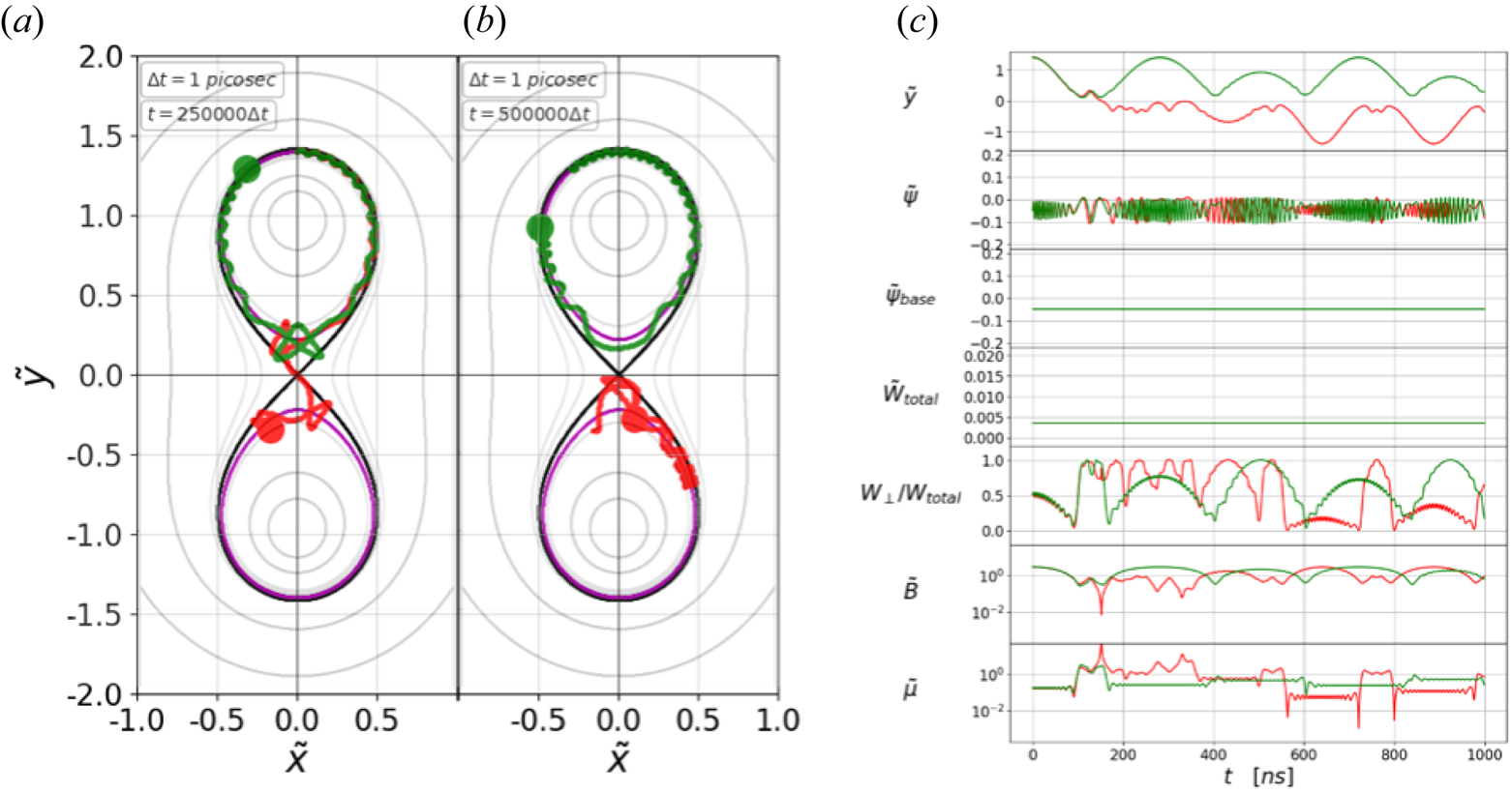
Figure 2. Two particles with the same invariants ($\tilde {\psi }_\text {base}=-0.05, \tilde {W}_\text {total}=0.0035$ ) are simulated in the TWM configuration. These particles start from the top of $\tilde {\psi }=-0.05$
 with $\tan ^{-1}{(v_y/v_x)}=45^\circ$
 (red) and $46^\circ$
 (green). The magenta field line indicates the location of $\tilde {\psi }_\text {base}=-0.05$
 . Traces of the particles are shown in (a) for $t=0\unicode{x2013}250\ {\rm ns}$
 and in (b) for $t=250\unicode{x2013}500\ {\rm ns}$
 . Temporal traces of various physical quantities of interest for the red and the green particles are shown in (c) from $t=0$
 to $1000\ {\rm ns}$
 as red and green lines, respectively.
There are two interesting phenomena to observe in this example, which are the main topics of this study, i.e. the magnetic moment shifts and the associated migrations. First, as can be seen from the last plot of figure 2(c), the particles’ normalized magnetic moments $\tilde {\mu }$ make seemingly random shifts to various values. The $\tilde {\mu }$
 shifts occur whenever the particle travels near the X-point, where the field gradient is large. This observation including its sensitivity to the initial injection angle, i.e. difference in green and red particles, is further detailed in § 4.
Second, a particle may jump to follow other closed field lines. For $\tilde {\psi }_\text {base}<0$ , the base field line is two closed circles separated by the separatrix, as indicated by the magenta lines in figure 2(a,b). A particle typically gyrates about and travels along the closed field line on one side. However, if the Larmor radius becomes large enough, due to occasional magnetic moment shifts, the particle can transport to the other closed field line in the TWM configuration, as can be seen with the red particle in figure 2(a). During this transport, due to the reversal of the magnetic field direction, the particle follows one cycle of the betatron orbit. This transport phenomenon is termed ‘migration’ in this study. The first temporal plot of figure 2(c) shows that the red particle migrates at $t\approx 100\ {\rm ns}$
 , that is, $\tilde {y}$
 becomes negative from positive, and stays on the negative side. Note that the green particle does not migrate, at least up to $t=1000\ {\rm ns}$
 in this example; however, it can eventually migrate to the other side as well for it satisfies the necessary condition for the migration, which is discussed in § 5.
4 Magnetic moment shift
We have observed that the behaviours of the $\tilde {\mu}$ shift are different for different initial injection angles with the same two invariants (see the $\tilde {\mu}$
 traces in figure 2c). This can be explained with an inhomogeneous magnetic field causing chaotic particle orbits (Büchner & Zelenyi Reference Büchner and Zelenyi1989; Numata & Yoshida Reference Numata and Yoshida2002, Reference Numata and Yoshida2003), which result in different realizations of $\tilde {\mu }$
 . Due to its chaotic behaviour, the statistical properties of the $\tilde {\mu }$
 shift are investigated.
4.1 Histogram of the magnetic moment
We first consider the overall consequences of the initial injection angles for the $\tilde {\mu }$ shift. This is done with seven particles whose invariants are the same, i.e. $\tilde {\psi }_\text {base}=-0.05$
 and $\tilde {W}_\text {total}=0.002$
 . All of them start from the top of $\tilde {\psi }=-0.05$
 , but with different initial injection angles from $0^\circ$
 to $30^\circ$
 with an interval of $5^\circ$
 .
.
Figure 3(a) shows histograms of $\tilde {\mu}$ for the seven particles obtained by simulating them up to $t=10\ {\rm ms}$
 . It clearly shows that the different initial injection angles all lead to the same histogram, while their individual realizations are different, as shown in figure 3(b). Although not shown here, many more cases with random positions and injection angles ($0$
 to $2{\rm \pi}$
 ) for the same invariant pair are simulated, and the resultant histograms are found to be identical. The same holds true for cases with different invariant pairs, and the invariant pair is the only factor that determines the shape of the histogram. Therefore, we can infer that the path, which a particle covers in a long time, is independent of the initial condition and distinguished by the invariant pair of the particle.
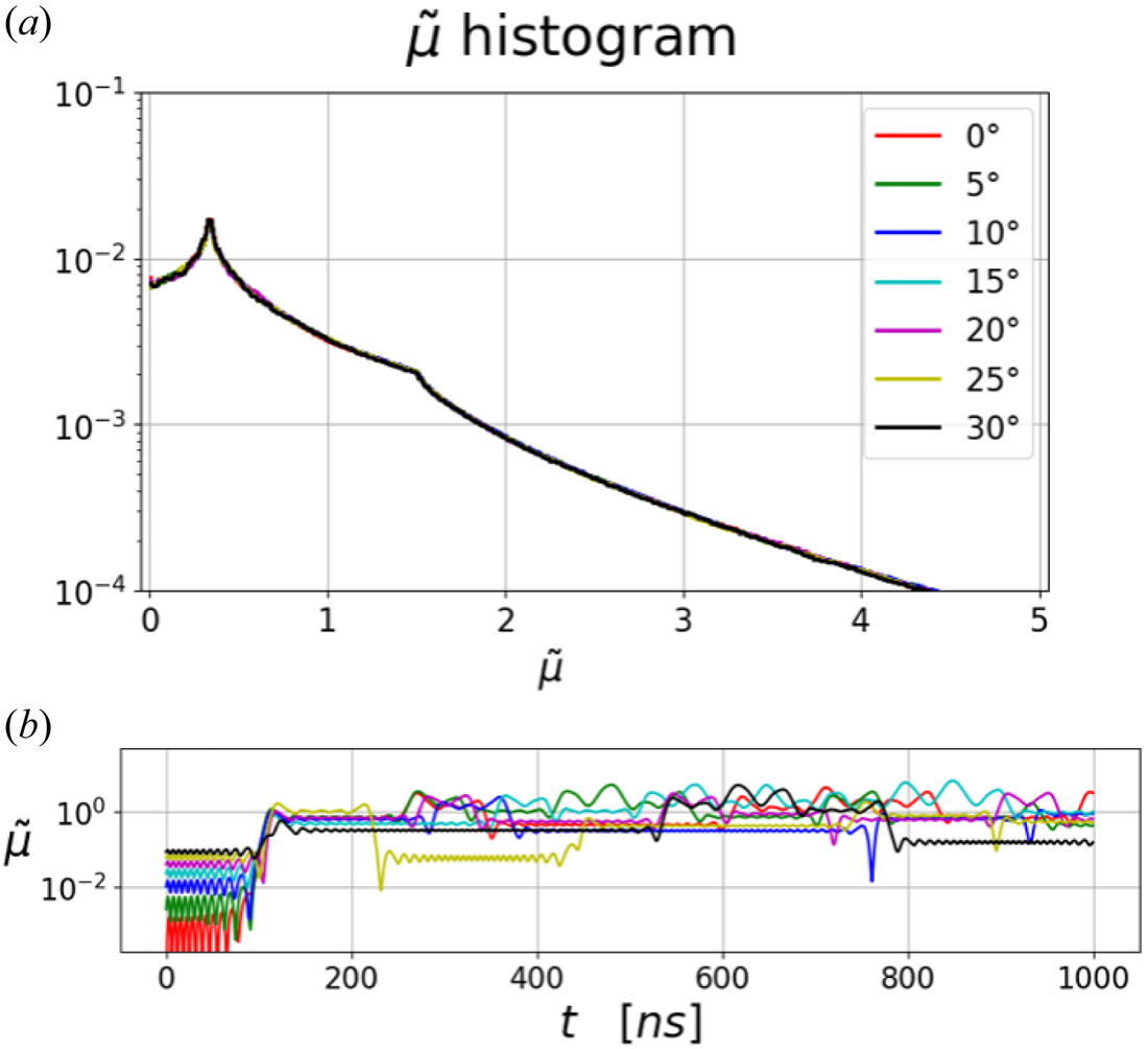
Figure 3. (a) Histograms of $\tilde {\mu }$ for seven particles obtained by simulating them up to $t=10\ {\rm ms}$
 . Invariant pairs of the seven particles are identical, i.e. $\tilde {\psi }_\text {base}=-0.05$
 and $\tilde {W}_\text {total}=0.002$
 . They start from the top of $\tilde {\psi }=-0.05$
 having different initial injection angles from $0^\circ$
 to $30^\circ$
 with a $5^\circ$
 interval. (b) Each realization of $\tilde {\mu}$
 for the seven particles from $t=0$
 to $1000\ {\rm ns}$
 , showing that they are all different while the histograms are the same.
4.2 Correlation between the current and next magnetic moments
Next, we statistically investigate how the current value of $\tilde {\mu}$ is correlated with the next one. Figure 4(a) shows the trajectory (red) of a single particle having the invariant values of $\tilde {\psi }_\text {base}=-0.05$
 (magenta) and $\tilde {W}_\text {total}=0.00225$
 with the initial injection angle of $\tan ^{-1}{(v_y/v_x)}=45^\circ$
 . We find that $\tilde {\mu }$
 shifts abruptly whenever the particle passes near the large gradient region around the X-point, indicated by the blue line in figure 4(a), which is the reference line connecting the positions of the two wires (cf. figure 1c). It can be seen clearly from figure 4(b) that the abrupt shifts of $\tilde {\mu}$
 coincide with the blue vertical lines that indicate the times when the particle passes the reference line. Thus, we define an expectation value of the $\tilde {\mu}$
 , denoted as $\langle \tilde {\mu } \rangle _k$
 , to be the arithmetic average of $\tilde {\mu}$
 values in between two consecutive ($k$
 th and $k+1$
 th) crossings of the reference line.
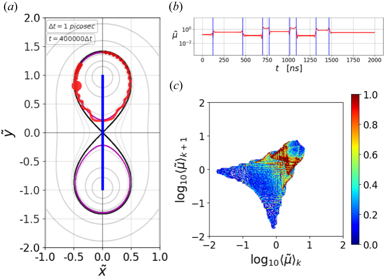
Figure 4. (a) Trajectory (red) of a single particle starting from the top with $\tilde {\psi }_\text {base}=-0.05$ (magenta), $\tilde {W}_\text {total}=0.00225$
 and $\tan ^{-1}{(v_y/v_x)}=45^\circ$
 from $t=0$
 to $400\ {\rm ns}$
 . The vertical reference line (blue) connects the positions of the two wires where the spatial gradient of the magnetic field is large (cf. figure 1c). (b) Temporal evolution of $\tilde {\mu }$
 from $t=0$
 to $2000\ {\rm ns}$
 , and the blue vertical lines indicate when the particles crosses the reference line, and (c) normalized two-dimensional histogram for $\langle \tilde {\mu } \rangle _k$
 (abscissa) and $\langle \tilde {\mu } \rangle _{k+1}$
 (ordinate) indicating the correlation between the two consecutive $\langle \tilde \mu \rangle$
 values.
This single particle is simulated up to $30\ {\rm ms}$ to obtain the correlation between $\langle \tilde {\mu } \rangle _k$
 and $\langle \tilde {\mu } \rangle _{k+1}$
 . This is visualized as a two-dimensional normalized histogram with $400\times 400$
 square bins in figure 4(c). As attested by the histogram, the behaviour of the $\langle \tilde \mu \rangle$
 shifts is not completely random, indicating that the next $\langle \tilde \mu \rangle$
 can be probabilistically predicted given a current $\langle \tilde \mu \rangle$
 , albeit with stochasticity. In addition, multiple simulations with the same pair of invariants are performed to conclude that the resultant histograms are independent of the initial injection positions or angles.
We have also investigated how different sets of the invariants affect the correlation between the current and next $\langle \mu \rangle$ . For this purpose, we introduce a new quantity, the ‘base energy’, defined as $\tilde {W}_\text {base}=\tilde {\psi }_\text {base}^2$
 . Basically, $\tilde {W}_\text {base}$
 is the normalized threshold energy for a particle to cross the separatrix, i.e. only if $\tilde {W}_\text {total}/\tilde {W}_\text {base}$
 is greater than unity can a particle cross the separatrix. Its role as the threshold and the physical meaning of $\tilde {W}_\text {base}$
 are derived and discussed in § 5. From here on, we use $\tilde {\psi }_\text {base}$
 and $\tilde {W}_\text {total}/\tilde {W}_\text {base}$
 as a pair of the two invariants to distinguish a particle.
Figure 5 shows the two-dimensional histograms illustrating correlations between the current and next $\langle \mu \rangle$ for different sets of the invariants. Figure 5(a–d) is of $\tilde {\psi }=-0.05$
 , while figure 5(e–h) is of $\tilde {\psi }=-0.20$
 with different values of $\tilde {W}_\text {total}/\tilde {W}_\text {base}$
 . The particles with a lower energy ($\tilde {W}_\text {total}/\tilde {W}_\text {base}=0.1$
 ) have the sharper histograms (figure 5a,e), meaning that the amounts of $\langle \mu \rangle$
 shifts are relatively small and the shifts are more predictable. This is because the particle travels more slowly, and the magnetic field change it feels is slower. The particles with $\tilde {W}_\text {total}/\tilde {W}_\text {base}=1.0$
 move faster and can reach the X-point. Hence, they can feel more rapid changes of the magnetic field, and so the histograms are wider (figure 5c,g). Therefore, we conclude that, in the TWM configuration, the magnetic moment shift is more stochastic for a higher energy since such particles travel faster and go closer to the large gradient region.
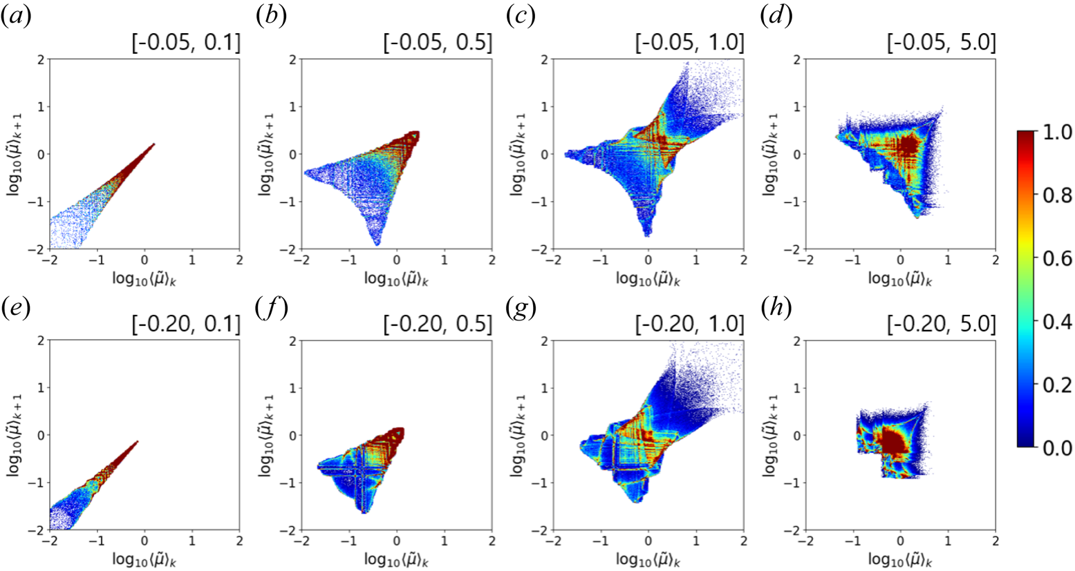
Figure 5. Normalized two-dimensional histograms for $\langle \tilde {\mu } \rangle _k$ (abscissa) and $\langle \tilde {\mu } \rangle _{k+1}$
 (ordinate) indicating the correlation between the two consecutive $\langle \tilde \mu \rangle$
 values with different pairs of the two invariants denoted as $[\tilde {\psi }_\text {base}, \tilde {W}_\text {total}/\tilde {W}_\text {base}]$
 on each plot.
5 Migration
As noted earlier, a normalized field line value $\tilde {\psi }$ less than zero corresponds to two separate closed field lines located above and below the magnetic X-point inside the separatrix (see magenta lines in figure 2a,b). Migration is defined, in this work, as the phenomenon where a particle jumps to follow the other field line, i.e. the sign of the $\tilde {y}$
 -position of a particle flips, with the same $\tilde {\psi }$
 in the TWM configuration.
5.1 Threshold energy for the migration
We find that probability of migration depends on the two invariants, and there is a minimum required energy. These findings can be well explained with a possible particle trajectory described by the effective potential (Kim & Cary Reference Kim and Cary1983). Since there is no $z-$ component of the magnetic field in the TWM configuration, we divide the equation of motion (3.1) into $xy$
 - and $z$
 -components to derive the effective potential as

Then, taking the $xy$ -component, we have

where

Note that the ‘base energy’ was defined earlier (see § 4) as $\tilde {W}_\text {base}=\tilde {\psi} ^2_\text {base}=W_\text {base}/W_0$ .
.
The total energy of a particle is the sum of the kinetic energy in the $xy$ -plane and the effective potential, i.e. $W_\text {total}=W_{xy}(v_x, v_y)+U_\text {eff}(x,y)$
 , which means that $U_\text {eff}$
 cannot exceed $W_\text {total}$
 . Therefore, a particle's trajectory is restricted to be within a certain range of $\tilde {\psi }_\text {base}$
 , where its minimum and maximum bounds, denoted as $\tilde {\psi }_\text {min}$
 and $\tilde {\psi }_\text {max}$
 , are
, are

This tells us that a particle with $\tilde {\psi }_\text {base}<0$ can have a trajectory outside of or on the separatrix only if $\tilde {W}_\text {total}/\tilde {W}_\text {base} \ge 1$
 . Only in this case may the particle cross the separatrix and the X-point. Therefore, this is precisely the necessary condition for migration; in other words, $\tilde {W}_\text {base}$
 is the threshold energy.
Figure 6(a–d) shows contour plots of $U_\text {eff}/W_\text {total}$ for different energies $\tilde {W}_\text {total}/\tilde {W}_\text {base}$
 with the same $\tilde {\psi }_\text {base}=-0.10$
 (magenta lines). This shows the two bounds, i.e. $\tilde {\psi }_\text {min}$
 and $\tilde {\psi }_\text {max}$
 , for the particle motion. It is impossible for a particle to travel into the region of $U_\text {eff}/W_\text {total} > 1$
 , depicted as the grey area. It clearly shows that the accessible area is divided into upper and lower sides, and the two sides are connected when $\tilde {W}_\text {total}/\tilde {W}_\text {base} \ge 1$
 . This means that migration is only possible when this condition is satisfied, which is the same conclusion discussed above.
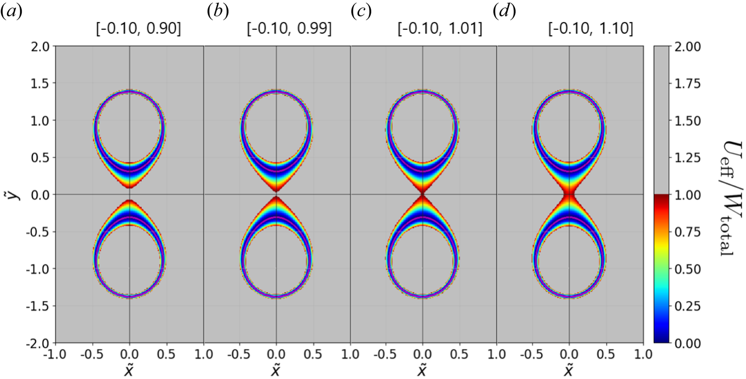
Figure 6. (a–d) Contour plots of $U_\text {eff}/W_\text {total}$ with various pairs of invariants denoted as $[\tilde {\psi }_\text {base}, \tilde {W}_\text {total}/\tilde {W}_\text {base}]$
 on each plot, showing that a particle can migrate to the opposite side of the closed field lines only if $\tilde {W}_\text {total}/\tilde {W}_\text {base} \ge 1$
 . Grey regions indicate inaccessible areas for the particle. Magenta lines correspond to $\tilde {\psi }_\text {base}=-0.10$
 .
.
A particle with $\tilde {W}_\text {total}/\tilde {W}_\text {base} \ge 1$ travels on one side of the TWM configuration, experiences the occasional magnetic moment shifts (discussed in § 4) and, eventually, it can have a Larmor radius large enough to cross the $\tilde {y}=0$
 axis to migrate to the other side. This is how the migration occurs, and it is significant for it represents a possibility of collisionless transport loss of particles that reside inside the separatrix in addition to a turbulence driven collisionless transport (Choi & Hahm Reference Choi and Hahm2022; Choi Reference Choi2023).
5.2 Migration confinement time (collisionless transport time scale)
We have recorded the times a particle spent in between the consecutive migrations, and histograms of such times are shown in figure 7 for $[\tilde {\psi }_\text {base}, \tilde {W}_\text {total}/\tilde {W}_\text {base}]$ equal to (a) $[-0.10, 1.20]$
 and (b) $[-0.10, 1.50]$
 . As attested by the figure, the times are distributed exponentially, indicating that migration is an almost memoryless phenomenon. There exists a sharp outlier in a very short time, which may be caused by the gyrating orbits of a particle very close to the X-point. The average time is termed as the ‘migration confinement time’, $\tau _\text {mig}$
 , and we have $\tau _\text {mig}=594\ {\rm ns}$
 and $275\ {\rm ns}$
 for figure 7(a,b), respectively. This quantity represents how probable migration is for a particle with a certain pair of the invariants. We see that the migration confinement time is shorter for a particle with a higher energy.
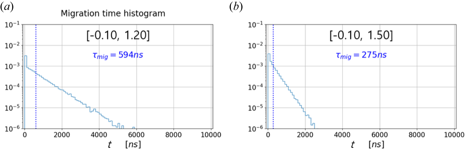
Figure 7. Histograms of time a particle spent in between the consecutive migrations for the invariant pair $[\tilde {\psi }_\text {base}, \tilde {W}_\text {total}/\tilde {W}_\text {base}]$ of (a) $[-0.10, 1.20]$
 and (b) $[-0.10, 1.50]$
 . Migration confinement time, $\tau _\text {mig}$
 , which is the average value from the histogram, is depicted in (a) and (b) with blue vertical dotted lines.
We have seen that collisionless transport is possible due to the magnetic moment shift as a particle with enough energy travels into the region of a large magnetic field gradient, such as around the magnetic X-point. Thus, we have estimated the normalized migration confinement time $\tilde {\tau }_\text {mig}=\tau _\text {mig}/\tau _0$ for 600 different pairs of the invariants such that the overall quantitative behaviour of $\tau _\text {mig}$
 can be empirically formulated. We have simulated a particle with six values of $\tilde {\psi }_\text {base}$
 , which are $-0.005, -0.010, -0.020, -0.050, -0.100$
 and $-0.200$
 . For each $\tilde {\psi }_\text {base}$
 , we have 100 different values of $\tilde {W}_\text {total}$
 from $\tilde {W}_\text {total}-\tilde {W}_\text {base}$
 equal to $0.01\tilde {W}_\text {base}$
 to unity.
Figure 8 shows the estimated $\tilde {\tau }_\text {mig}$ as a function of (a) $\tilde {W}_\text {total}-\tilde {W}_\text {base}$
 , i.e. how much excess energy a particle has, and (b) $\tilde {W}_\text {total}/\tilde {W}_\text {base}-1$
 , i.e. how much fractional excess energy with respect to the base energy $\tilde {W}_\text {base}$
 (or the threshold energy) a particle has. We now construct an empirical expression for $\tilde {\tau }_\text {mig}$
 based on the numerical results. As can be seen from figure 8, the trend follows two different power laws. First of all, there seems to be, from figure 8(a), a converging power law at large $\tilde {W}_\text {total}-\tilde {W}_\text {base}$
 with different values of $\tilde {\psi }_\text {base}$
 ; thus, we introduce a $\alpha (\tilde {W}_\text {total}-\tilde {W}_\text {base})^{\beta }$
 factor in the formula. Second, from figure 8(b) we observe a similar slope for different values of $\tilde {\psi }_\text {base}$
 for small $\tilde {W}_\text {total}/\tilde {W}_\text {base}-1$
 with different offsets. Therefore, we include a $[({\tilde {W}_\text {total}}/{\tilde {W}_\text {base}}-1)^{\gamma } - \tilde {W}_\text {base}^{\delta } + 1]$
 factor in the formula as well. Together, we have

where the fitting parameters $\alpha, \beta, \gamma$ and $\delta$
 are obtained using the numerically obtained $\tilde {\tau }_\textrm {mig}$
 . The black lines in figure 8(a,b) are the fitted lines, which show good agreements.
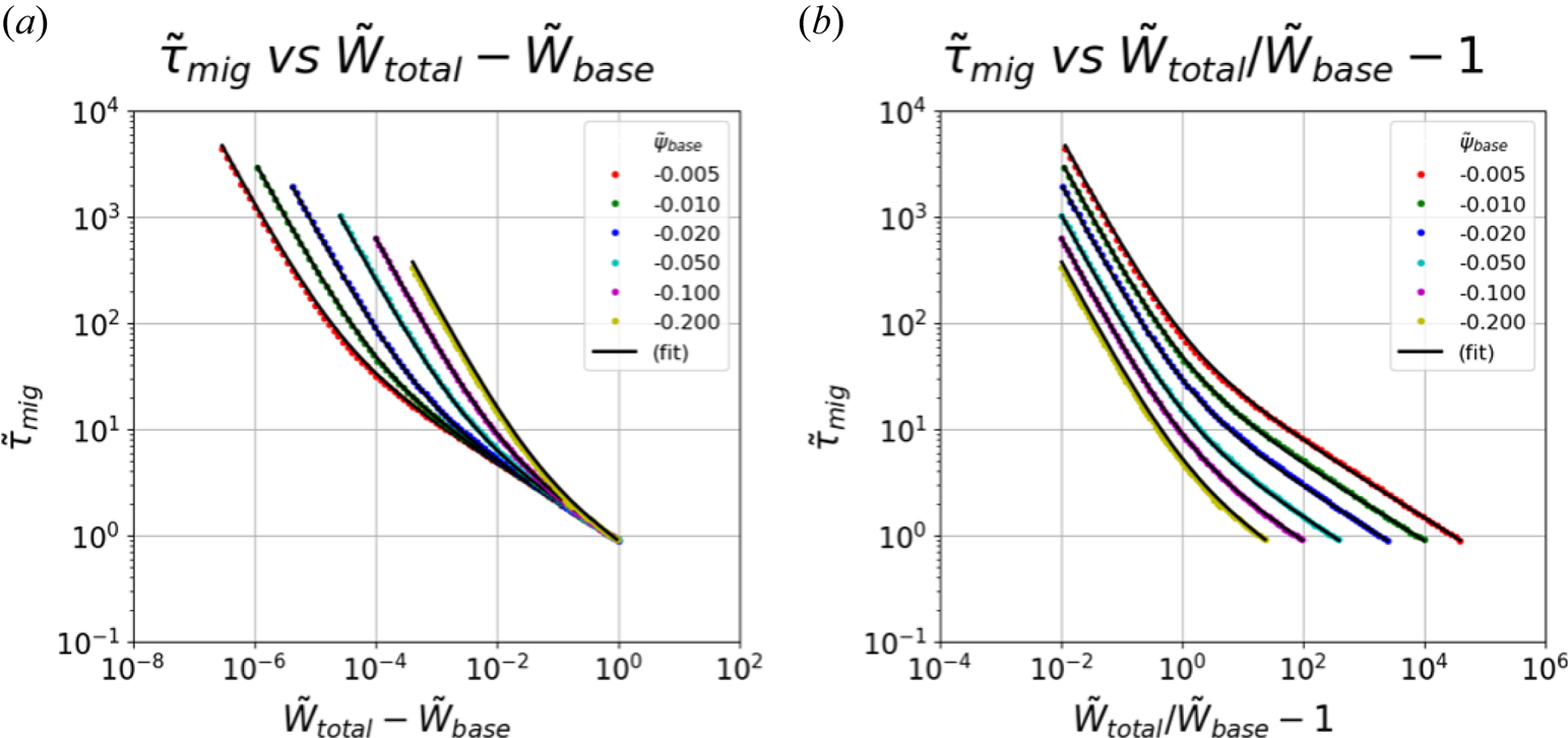
Figure 8. Estimated normalized migration confinement time $\tilde {\tau }_\text {mig}$ from 600 different pairs of $\tilde {\psi }_\text {base}$
 and $\tilde {W}_\text {total}$
 as a function of (a) $\tilde {W}_\text {total}-\tilde {W}_\text {base}$
 and (b) $\tilde {W}_\text {total}/\tilde {W}_\text {base}-1$
 . We have simulated a particle with six different values of $\tilde {\psi }_\text {base}$
 , which are $-0.005, -0.010, -0.020, -0.050, -0.100$
 and $-0.200$
 . For each $\tilde {\psi }_\text {base}$
 , we have 100 different values of $\tilde {W}_\text {total}$
 . Black lines are the fitted lines obtained by the empirical expression (5.5).
Equipped with the empirical expression (5.5), we show the quantitative trend of $\tilde {\tau }_\textrm {mig}$ as a function of $\tilde {\psi} _\textrm {base}$
 and $\tilde {W}_\textrm {total}$
 in figure 9. Note that we use the absolute value of $\tilde {\psi} _\textrm {base}$
 since the confined particles have $\tilde {\psi} _\textrm {base}<0$
 . It is clear that $\tilde {\tau }_\textrm {mig}$
 is finite only when $\tilde {W}_\textrm {total} > \tilde {W}_\textrm {base} = \tilde {\psi }_\textrm {base}^2$
 as a particle cannot migrate otherwise. The value of $\tilde {\tau }_\textrm {mig}$
 decreases with increasing $\tilde {W}_\textrm {total}$
 and decreasing $|\tilde {\psi} _\textrm {base}|$
 , which behaviours are consistent with our intuition. We emphasize that our results can be readily applied to any other charged particle species since we have used the normalized quantities.
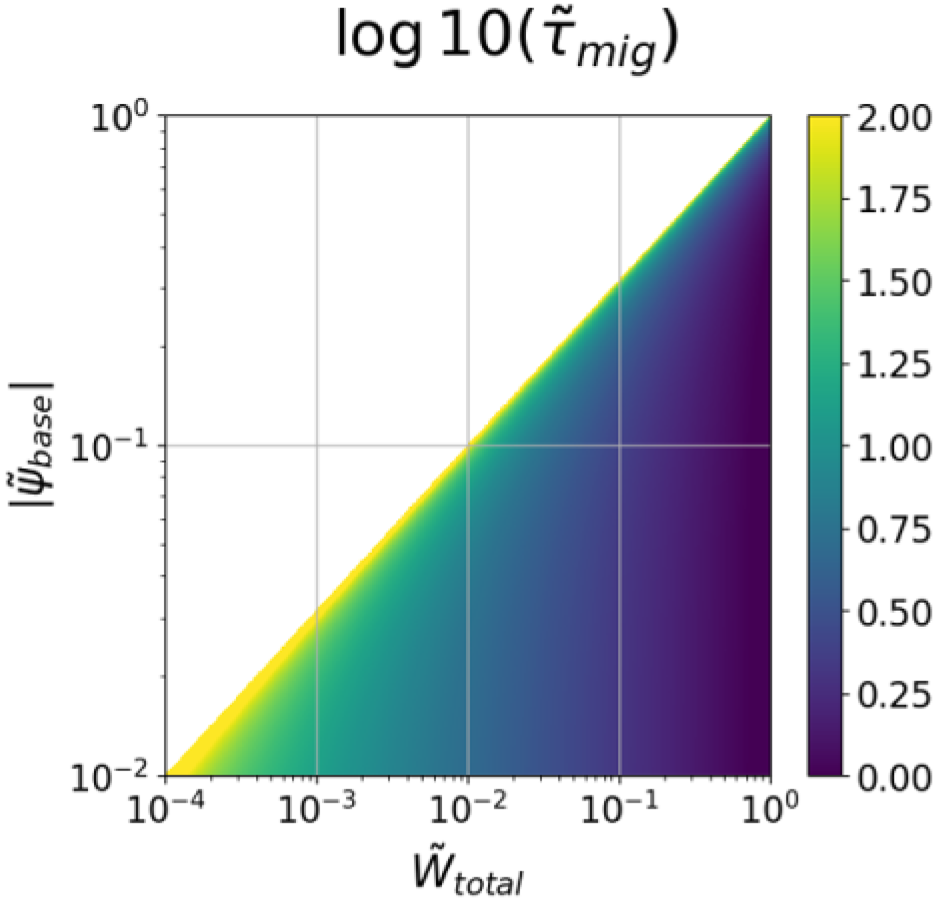
Figure 9. Value of $\tilde {\tau }_\textrm {mig}$ as a function of $|\tilde {\psi} _\textrm {base}|$
 and $\tilde {W}_\textrm {total}$
 obtained by the empirical expression (5.5), showing the quantitative trend of $\tilde {\tau }_\textrm {mig}$
 with the two invariants of a particle.
5.3 Application to tokamak plasmas
This migration phenomenon causes particles to become completely lost from the system if there is a loss boundary on the other side of the TWM configuration, such as a divertor in a tokamak. To investigate how relevant this collisionless transport can be, we create a similar environment, although it is crude for there are no axial (or toroidal) magnetic fields, as in a tokamak with the independent system quantities of $I=100\ {\rm kA}$ and $\ell =1.0\ {\rm m}$
 with a deuteron species $(q/m=4.79 \times 10^{7}\ \textrm {C}\ \textrm {kg}^{-1})$
 . We then have $\tau _0=6555.33\ {\rm ns}$
 and $W_0=9584.85\ {\rm eV}$
 and, therefore, $\Delta {t}=1\ {\rm ns}$
 is used for this simulation. We randomly place 30 000 deuterons on the upper side of $\tilde {\psi }_\textrm {base}=-0.1$
 with isotropically distributed initial injection angles. These ions are initialized with a Maxwellian distribution having $T=2/3\langle W_\textrm {total} \rangle = 100\ {\rm eV}$
 (see figure 10d). Since all the ions have $\tilde {\psi }_\textrm {base}=-0.1$
 , we have $W_\textrm {base}=95.85\ {\rm eV}$
 , which means only some of the deuterons with a high enough energy may migrate to the lower side and eventually be lost to the loss boundary (virtual divertor) located at $\tilde {y}=-0.5$
 .
.
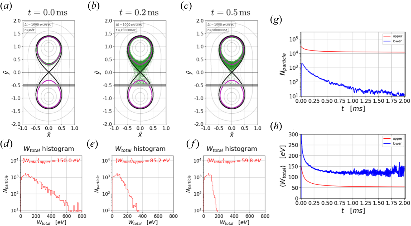
Figure 10. An example of particle losses due to the collisionless migration phenomenon with the loss boundary, acting as a divertor in a tokamak, located at $\tilde {y}=-0.5$ (thick grey horizontal line). Initially, 30 000 Maxwellian deuterons (green dots) are randomly placed on $\tilde {\psi }_\textrm {base}=-0.1$
 (magenta line) on the upper side of the TWM configuration. (a–c) Show the spatial distribution of deuterons at times $t=0.0, 0.2$
 and $0.5\ {\rm ms}$
 , respectively. (d–f) Are the histograms of $W_\textrm {total}$
 at these times. (g,h) Show temporal evolutions of the number of particles and $\langle W_\textrm {total} \rangle$
 for the upper and lower sides, respectively.
Figure 10(a–c) shows the spatial distribution of deuterons (green dots) at times $t=0.0, 0.2$ and $0.5\ {\rm ms}$
 , respectively. Figure 10(d–f) shows the $W_\textrm {total}$
 histograms at these times. It is clear that, as time progresses, the high tail of the distribution is quickly lost to the virtual divertor since the migration confinement times of the high energy particles are shorter. This can be also seen with the decreasing average energy of the particles, denoted as $\langle W_\textrm {total} \rangle$
 . By the time $t=0.5\ {\rm ms}$
 , most of the deuterons with $W_\textrm {total} > W_\textrm {base}$
 have migrated to the lower side, and only the low energy deuterons remain confined on the upper side. Figure 10(g,h) shows temporal evolutions of the number of particles and $\langle W_\textrm {total} \rangle$
 , respectively, for the upper (red) and lower (blue) sides of the TWM configuration. We note that, even at around $t=2.0\ {\rm ms}$
 , there exist particles migrating to the lower side due to the random nature of the phenomenon. Through this example we can see that, even if particles are following the base field line inside the separatrix, they may migrate to the other side and become lost to a boundary.
As mentioned earlier, this result may not be directly applied to tokamak edge physics as we lack not only the axial (toroidal) magnetic fields but also collisions, which restore a Maxwellian distribution. Nevertheless, as a typical transport time and an ion collision time in a tokamak are of the order of a few to tens of ms (Wesson Reference Wesson2011), we see that the collisionless transport time scale associated with the migration is much faster. If there were axial magnetic fields, they would have slowed down the migration transport, while the collisions would have escalated it. Thus, the migration may play a non-negligible role for determining an edge transport time scale as well as a radial profile in the scrape-off-layer region of a tokamak.
6 Summary and conclusion
We have numerically investigated a collisionless single charged particle motion in the TWM configuration whose magnetic geometry follows a Cassini oval with a magnetic X-point. We have focused on the magnetic moment shift and its subsequent transport as a particle travels near the X-point, where the conservation of the magnetic moment is no longer valid, i.e. a region with large spatial gradients of the magnetic field magnitude.
From the Lagrangian analysis, two system invariants which can be used to distinguish particles are identified, i.e. the total kinetic energy and the base field line value. We find that, although the particles’ initial conditions are different, causing various realizations of chaotic magnetic moment shifts, their long time trajectories eventually cover the same area as long as their pairs of the invariants are the same. Detailed numerical analyses show that seemingly random magnetic moment shifts are, in fact, statistically well behaved, that is, knowledge of the current magnetic moment allows us to predict the next one with a certain probability distribution, which is completely determined by the two invariants.
We have observed that, when the magnetic moment shifts to a larger value, leading to a larger Larmor radius, the particle probabilistically crosses the separatrix to follow the base field line on the other side of the TWM configuration. This phenomenon is denoted as migration in this work. When a migration occurs, the particle can no longer be considered confined inside the separatrix, resulting in a collisionless loss of the confined particles. Using the two-dimensional effective potential, we have found a necessary condition for migration that the total energy of a particle must be larger than a threshold energy determined by one of the invariants, i.e. the base field line value.
As evidenced by the exponentially distributed separatrix-crossing time, migration is a memoryless random process. Therefore, we have estimated the average crossing time, the migration confinement time, and it is found to be only a function of the two invariants. Since the migration confinement time is relevant to the collisionless transport, we have formulated its empirical expression. This has been done by simulating particles with 600 different pairs of the invariants from which we can estimate the migration confinement time.
To examine whether or not the migration phenomenon investigated in this work is relevant for the edge transport of tokamak plasmas, we have simulated particles with similar environments to that in a typical tokamak. Albeit our results may not be directly used to explain the edge transport due to rather crude simplifications, we have found that the migration has a certain degree of potential for determining an edge transport time scale and a radial profile in the scrape-off-layer region of a tokamak.
With an in-depth physical intuition of how a single particle behaves around the magnetic X-point, we plan to investigate such transport phenomena with particle-in-cell simulations, where self-consistent fields are properly treated, with finite collisions and additional external fields.
Acknowledgements
Editor Cary Forest thanks the referees for their advice in evaluating this article.
Funding
This work was supported by the National R&D Program through the National Research Foundation of Korea (NRF) funded by the Ministry of Science and ICT (Grant Nos. RS-2022-00155917 and NRF-2021R1A2C2005654).
Declaration of interest
The authors report no conflict of interest.
Data availability statement
The data that support the findings of this study are available from the corresponding author upon reasonable request.
Author contributions
B.A., Y.L. and Y.-C.G derived the theory, and B.A. performed the simulations. All authors participated in discussions and contributed to the writing and editing of the manuscript.


 Open access