


Introduction
The series of five Landsat spacecraft, of which the first was launched in July 1972, opened up new opportunities for glaciological studies that have proved especially valuable in remote areas. Landsats 1, 2, and 3 provided Multispectral Scanner (MSS) coverage of Antarctica (north of the satellite limit at about lat. 81°S). The MSS instrument has a picture-element (pixel) resolution of about 80 m, and operated mainly in the visual and “near” infra-red wavelengths.
Landsats 4 and 5 provided both MSS and Thematic Mapper (TM) images. In this paper we discuss TM images from Dronning Maud Land that were obtained by Landsat-5 in 1985. The images have six spectral reflective bands (TM1-5, 7) with a pixel resolution of about 30 m, and a thermal band (TM6) with a pixel resolution of about 120 m. The wavelengths covered by these bands (e.g. Markham and Barker 1986) are shown inTable I .
TM bands 1–4 are in the visual and “near” infra-red wavelengths and partly overlap the MSS bands, whereas TM bands 5 and 7 are in the reflective infra-red. The TM data are more valuable for ice-sheet studies than MSS data because the spatial resolution is three times higher, and the additional bands in the infra-red give more information on snow, ice, clouds, and water.
The Landsat Data
Fifty-seven images from central and western Dronning Maud Land were acquired by Landsat-5 between November 1984 and March 1986. Most of these show low cloud cover and were recorded both by the MSS and by the TM instruments in the 1984–85 summer season, to coincide with a dedicated ground programme that was part of the Norwegian Antarctic Research Expedition 1984–85. Two scenes, No. 5034407520 (recorded on 8 February 1985) and No. 5036207394 (recorded on 26 February 1985) are discussed in this paper (Fig. 1).

Fig. 1. Index map, showing the location of the study area and the two Landsat images discussed in this paper. The dotted lines show the land boundary of the continent.


Fig. 2a. Quad 1 (upper left quadrant) of Landsat scene 5034407520.
(a) Colour-coded brightness temperatures (BTs), determined from TM-band 6 data. BTs range from around −12°C (red) to −30°C (dark green), and relate closely to elevation. Arrows point to warm areas on nunataks facing the Sun (lower right), and to lakes (white, left of centre); the lakes are the warmest features in the image, with BTs of −8° to −9°C. The temperature scale below the figure also applies to Figures 3a and 4a. The picture is 90 km wide, north toward upper left.

Fig. 2b. (b) Contour map, showing air temperatures in °C 2 m above the snow surface (heavy solid lines), and elevation contours (dotted lines). The topography for this figure and for Figures 3b and 4b is based on Norsk Polarinstitutt 1:250 000 scale maps, with a 100 m contour interval. Elevation contours are approximate in most of the area, because of the scarcity of geodetic ground control.
Data Processing and Digital Enhancement
The present discussion concerns digitally enhanced images. Linear stretches were applied to individual TM bands after inspection of the histograms of relative reflectivity. Special stretches and (where appropriate) filters were applied to bring out detail in the snow and ice. Stretches in bands 5 and 7 may be severe, because most of the picture information is concentrated in the low-reflectivity region of the histograms. Saturation chiefly affects band 1, and therefore this band is not discussed here.
A full Landsat scene covers approximately 180 km × 180 km. The TM data are divided into four quarter-scenes (quads) numbered 1, 2, 4, and 3, reading clockwise from the upper left quad.
Reference Orheim and LucchittaOrheim and Lucchitta (1987) presented examples of the variety of glaciological information available from TM data.
They showed that the lower bands are most useful for recognizing surface topography, and that bands 5 and 7 are best for distinguishing different types of snow and ice. Here we carry the procedure further, and show how the classification of features is improved by digitally manipulating the data from different TM bands. Results of three types of processing are presented:
(1) Calculations of brightness temperatures from the digital numbers (DN) of TM band 6 for each pixel of the scene acquired on 8 February 1985, and colour-coding of the temperatures.
(2) Calculations of principal components (PCs) for this scene by a statistical technique for selecting the sub-space in which most of the data variance lies (Reference Haralick, Fu and ColwellHaralick and Fu 1983, Reference Podwysocki, Segal and ColwellPodwysocki and Segal 1983). We used the reflective TM bands 2, 3, 4, 5, and 7, so that the PCs became a five-dimensional vector. PCs attempt to maximize the amount of image variation in a minimum number of components, and they are calculated by subtracting or adding proportions of each band for each component. Distinctions between surface materials may thus be emphasized, but the physical interpretation of a PC image is not always clear.
(3) Ratios of pairs of the reflective bands and composite images created from the ratios that give the most contrast. Ratioing partly eliminates the effects of brightness changes related to topography and the angle of illumination; therefore it emphasizes reflectance differences related to the physical properties of the surface.
Image Interpretation
General remarks
The basic physics of remote sensing of snow and ice in the TM bands is well established. The spectral reflectivity of snow depends on grain-size and shape, near-surface liquid-water content, surface roughness, impurities, and the angle of solar incidence. Various models have been developed for calculating the snow albedo (e.g. Reference Smith and ColwellSmith 1983). Reflectivity in snow generally decreases with increasing wavelength in the visual and “near” infra-red, and variations with wavelength in the albedo of snow, firn, and ice are broadly parallel (Reference Qunzhu, Meisheng, Xuezhi, Fengxian, Xianzhang and WenkunQunzhu and others 1984). Snow albedo decreases with increasing grain-size at wavelengths above 0.7 μm, but it varies little in the wavelengths below this value (Reference Choudhury and ChangChoudhury and Chang 1981). Thus grain-size variations do not show in TM bands 1, 2, and 3. By contrast, TM bands 5 and 7 discriminate well between snow, ice clouds, and water clouds; in these bands, albedoes of the three features increase in the order given (Reference DozierDozier 1985).
Surface temperatures
TM band 6 records radiation at about 11 μm. This band lies in an atmospheric window that is transparent to water vapour. Terrestrial black-body radiation at temperatures in the range −25° to 0°C reaches its maximum near this wavelength.
Reference Markham and BarkerMarkham and Barker (1986) provided data for calculating ground temperatures from the digital numbers recorded at the satellite. The spectral radiance, Lλ, is given in mW cm−2 ster−1 μm−1 from the following equation:
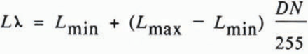
where L min and L max are calibration constants given as 0.1238 and 1.5600 mW cm−2 ster−1 μm−1 respectively, and DN is the observed digital number for each pixel, ranging from 0 to 255. These constants apply to data acquired after 15 January 1984.
The effective brightness temperature T, in K, of the viewed Earth-atmosphere system can then be calculated from Lλ according to the following equation:

Markham and Barker (1986) gave K1 = 60.776 mW cm −2 ster−1 μm–1, and K2 = 1260.56 K. They also stated that these numbers are the pre-launch calibration constants.
Figures 2a, 3a, and 4a show the computed brightness temperatures of quads 1, 2, and 4 recorded at the satellite at 07.52 GMT on 8 February 1985. Generally the brightness temperatures decrease with increasing elevation, and the effects of material reflectivity and the incidence angle of the Sun are superimposed on the elevation effects, so that the highest temperatures occur on surfaces of low albedo facing the Sun. Orheim and Lucchitta (1987) discussed some of these effects, which had been observed in the TM6 data. Here we explore whether the brightness temperatures correspond to ground observations.
We were able to reconstruct the ground-temperature distribution and to compare it with the satellite-measured temperatures because the Norwegian Antarctic Research Expedition 1984–85 operated a meteorological station on a snow-field (71°53’S, 5°10’E; 1600 ma.s.l.) and observed temperatures from 17 January to 14 February 1985 (Fig. 5a), both at the station and at many other locations (personal communication from T. Eiken). The station was about 10 km east of the image area of quad 2 (Fig. 3a), close enough to give representative values. Weather observations at 08.00 GMT on 8 February 1985 included the following: (at 2 m above the surface) air temperature: −12°C, and wind: 13 ms−1 from south; clouds: 0; precipitation: 0; and visibility: >50 km.
Mobile field parties measured air temperatures 2 m above the surface of the snow-field, at seven sites within quad 2 (Fig. 3b), from 19 January to 9 February 1985, typically over a 3d period (personal communication from T. Eiken). The sites range from 1380 to 2680 m in elevation. Temperature observations were also made at six sites, ranging in elevation from 50 to 2700 m, outside the area shown in this scene.
Air temperatures were linearly related to elevation. Observed temperature gradients for six sites, differing by >400 m in elevation from that of the meteorological station, ranged from 0.5°C/100m to l.l°C/100m. The mean gradient was 0.7°C/100m, and the gradients of the sites with the largest difference in elevation from that of the meteorological station were closest to this value. Using this gradient, we extrapolated the observations in order to construct maps of the air temperature 2 m above the surface for quads 1, 2, and 4 at 08.00 GMT for 8 February 1985 (Figs 2b, 3b, 4b). Comparison of extrapolated temperatures with measured temperatures indicates that the maps reproduce air temperatures over the large featureless snow areas to ±3°C.
One further set of ground temperatures is available. Water bodies, including 14 lakes as large as 3km2 in surface area, were observed in several places at about 100 m elevation in quad 1 (Orheim and Lucchitta 1987). Each lake had an albedo of about 0 in the six reflective bands. Their temperatures must have been 0°C or slightly lower if the water surface was covered by an ice layer (which was probably thin, because it was visually transparent). Pixel DN values for one of these lakes are given in Figure 6.
Observations at an ice-free site (Fig. 5b) demonstrate the more complex temperature variations over rock. The site was near the meteorological station. Its temperatures as recorded at the time of the satellite pass were −2.5°C below the gravel surface (under rock), −5.5°C at the surface (at the base of vegetation), and −6°C in the air 15 cm above the surface. These values clearly show the influence of the positive-radiation balance for low-albedo surfaces facing the Sun. On the other hand, on this clear day, areas in shadow had much lower surface temperatures (Fig. 3a). The present comparison of image and ground temperatures is restricted to areas of low relief where ground temperatures are homogeneous over large extents, making it easy to match pixel and ground data. We do not have sufficient field data to attempt to reproduce the greatly varying ground temperatures within the mountains and over blue-ice fields.

Fig. 3a. Quad 2 (upper right quadrant) of scene 5034407520.
(a) Colour-coded brightness temperatures, determined from TM-band 6 data. The areas in shadow behind the mountains are the coldest (dark blue and purple). The warm areas in the centre of the image are bare rock outcrops of Jutulsessen (largely white), lakes (red), and various blue-ice fields (orange). The latter are formed on the lee (west) side of nunataks and rock ridges and other topographic forms that interrupt drifting snow; the blue-ice fields align with the prevailing wind direction. Note also the cold areas in the snow-fields below the mountains, probably caused by cold air from the inland ice sheet flowing down along the ice streams and glaciers. The picture is 90 km wide, north toward upper left.

Fig. 3b. (b) Contour map, showing air temperatures in °C 2 m above the snow surface (heavy solid lines), and elevation contours (dotted lines). Locations of air-temperature observations are shown by x.
The satellite recorded the exo-atmospheric radiation from the ground. To correlate its measurements with those on the ground, we must consider two principal variables: (1) the relation between the measured air temperature and brightness temperatures, and (2) the amount of atmospheric absorption.
Scene 5034407520 was collected under cloud-free conditions, without detectable haze in the atmosphere, with a solar elevation angle of 22.1°, and during rising temperatures that indicate a slightly positive radiation balance for level snow surfaces. Strong winds at the time of image acquisition (13 ms−1, the strongest recorded by the expedition) imply an efficient heat exchange between the snow surface and the air. Data for similar conditions (e.g.Reference Vinje Vinje 1975) show snow-surface and air temperatures to correspond within 1–2°C. Therefore we assume that our measured snow and air temperatures were equal. Brightness temperatures are the product of the ground temperature and emissivity. At TM-band 6 wavelengths, the surface approximates a black body, and snow emissivity probably deviates little from unity. That the emissivity at the thermal band is constant is supported by observations that show marked patterns on the snow surface in the infra-red reflective bands 5 and 7 (see below). These patterns probably reflect different snow-surface properties, yet the patterns are not visible on thermal band 6 in the same area.

Fig. 5a. Fig. 5a. Mean daily air temperature at snow-field at 1600 m elevation, 17 January —14 February 1985. See text for the location of the measurements.

Fig. 5b. Fig. 5b. Ground and air temperatures recorded above rock near the same snow-field, 8–11 February 1985 (fromReference Somme S⌀mme 1986).
The recorded brightness temperature depends also on atmospheric absorption. The Landsat scene investigated contains a small group of what are probably alto-cumulus clouds (Orheim and Lucchitta 1987); the effect of these clouds can be seen as a brightness-temperature reduction of about 2°C. We assume that few other large atmospheric absorption effects existed, in particular because the low temperatures permit only a low water-vapour content. Atmospheric absorption over Antarctica should be less than that over more temperate latitudes, so that any constant calibration compensating for atmospheric absorption should, at this location, give rise to errors on the warm side.
Bearing in mind the potential errors discussed above, we conclude that the temperature maps (Figs 2b, 3b, and 4b) should reproduce the real near-surface temperatures of level snow to ±4°C. However, the comparisons of satellite brightness temperatures with measured surface temperatures (Figs 2a, 3a, and 4a) show that the brightness temperatures for the coldest snow areas are about 20°C too low, whereas the temperatures for the water bodies appear to be 8°C too low. These deviations are too large to be physically plausible. In general, the changes in brightness reflect those in the near-ground temperatures, but the brightness temperatures are too low and have a gradient that is too high.Table II is a summary of the results for the quads investigated. The DN values in the table exclude those representing less than 0.1% of the total number of pixels (see also Fig. 7), in order to eliminate spurious information. However, this also excludes the values for the small water bodies in quad 1, which have DN values as high as 72 (Fig. 6).

Fig. 6. Fig. 6. Pixel DN values for a lake of ≈2 km diameter at the edge of Jutulstraumen in quad 1, scene 5034407520. DN values of 67–72 in the larger circled area represent water which is possibly covered by a very thin layer of ice. Lower DN values in the central part of the lake (the smaller circled area) result from a cover of snow and ice. Such partial cover was commonly observed on the lakes.
These results expand the temperature range of the Landsat-5 TM-band 6 radiometric calibration undertaken in June 1984 by Reference Schott and VolchokSchott and Volchok (1985); their range comprised surface temperatures between approximately 12° and 35°C. They found that satellite-predicted and ground temperatures agreed at about 22°C, but that the sensor had a systematic gain error of 1.43, causing the higher temperatures to be given as increasingly too warm. They suggested that this error was produced by moisture accumulation in the instrument. Markham and Barker (1986) also noted that the post-launch calibration constants may differ from the pre-launch constants used in (equ.2). Our results indicate that the instrument has a gain of 1.63, i.e. about 20% higher than that given by Schott and Volchok (1985).

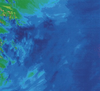
Fig. 4a. Quad 4 (lower right quadrant) of scene 5034407520 (a) Colour-coded brightness temperatures, determined from TM-band 6 data. The coldest areas (dark blue and purple) show BTs of −40°C. Note that the surface-snow patterns seen in TM bands 5 and 7 (fig. 8 in Orheim and Lucchitta 1987) and reflected in PC2 (Fig. 10) do not show in the BTs. Note also the small-scale variations in brightness temperatures of the snow surface above 2300 m elevation (Fig. 4b). The picture is 90 km wide, north toward upper left.

Fig. 4b. (b) Contour map, showing air temperatures in °C 2 m above the snow surface (heavy lines, dashed where located approximately), and elevation contours (dotted lines).

Fig. 7. Fig. 7. TM-band 6 DN frequencies for quads 1, 2, and 4 of scene 5034407520. Note different vertical scales. The differences in DN frequency distribution demonstrate the differences in elevation and radiance between the quads. Quad 1 contains the lowest and warmest areas of the scene, including water bodies and blue-ice fields at low elevations. Quad 2 covers the largest elevation intervals (Table II), and also includes most of the nunataks within the scene. These show a large range of £Ws, depending upon inclination to the Sun. Quad 4 is the most homogeneous and covers mostly high-elevation snow areas with low DN values.
A new temperature-contour map is shown in Figure 8. For its preparation we used our ground-temperature end members for the imaged area (0°C for lakes and −20°C for the coldest areas) and apportioned the radiance measured by TM band 6 to this temperature range. This map portrays the relative temperature variations as sensed by the satellite instrument, but it has temperature values that more realistically reflect the actual temperatures on the ground.
Table III gives pixel DN values and the corresponding revised brightness temperatures shown in Figure 8. We recommend additional ground-truth testing to clarify whether this Table can generally be used for estimating <0°C surface temperatures from DNs measured by Landsat-5.

Fig. 8. Fig. 8. Entire scene of 5034407520, showing temperature contours at 2°C intervals. The temperatures are calculated from TM-band 6 radiance values so as to reflect known temperature end members on the ground. Temperatures range from 0°C (white) to −23°C (dark blue), as shown by the temperature scale. The picture is 180 km wide, north toward upper left.

We conclude that the TM-band 6 data faithfully reproduced the relative temperature variations within a scene but had large errors in absolute temperatures. The brightness-temperature maps also show variations in surface temperature which we cannot test by ground truth, but Which we believe are real. The most important of these are probably related to variations in inclination and reflectivity, and were described previously. We also note the effects of cold air flowing down the ice streams (e.g. Figs 3a and 8) and detailed variations in snow temperatures over the inland plateau (Figs 4a and 8), which must have other causes.
Principal component technique
PCs are generally superior to individual bands or combinations of bands for displaying certain characteristics of a scene. Table IV gives the eigenvalue matrix and per cent variance of each PC of quad 4. The table shows that most of the information from the scene is contained in PCs 1–3. PCs 4 and 5 contain mostly noise and systematic image defects such as striping.
1. Topography
Figure 9a shows TM band 4 of part of quad 4 of scene 5034407520. Figure 9b shows PCI for the same area. A comparison of these figures shows that PCI, which reflects information common to all bands, is best for highlighting the topography of the inland ice sheet. Table IV also shows that PCI is dominated by the signal in TM bands 2, 3, and 4, whereas PC2 contains mostly information from TM bands 5 and 7. This observation confirms that of Orheim and Lucchitta (1987), who noted that TM bands
2, 3, and 4 are best for observing topographic variations in the glacier surface, whereas TM bands 5 and 7 show the physical properties of the surface.
PC1 reveals rolling topography in the south-east quadrant of quad 4, with wavelengths ranging mostly from 1.5 to 2.5 km. In Figure 9c we trace the ridge crests, a rendition that also emphasizes the intervening smooth areas. The digital numbers of PC1 show large variations across the waves, even though the regional slopes over the inland ice sheet in this area are between only 1 : 200 and 1 : 100 (0.3° and 0.6°). These waves are not parallel to the ice-surface contours. Instead, the majority are nearly at right angles to the solar azimuth, and aligned at right angles to the main wind direction.
Obviously these waves are accentuated in the direction of Sun incidence, which is supported by the observation that some marked topographic features aligned with the solar azimuth do not show at all. The visibility of the waves may also be enhanced by wind effects which cause accumulation rates to vary (Reference Gow and RowlandGow and Rowland 1965) and by changes in the physical properties of the snow surface across the waves. However, the wind patterns seen in bands 5 and 7 (and PC2) are at diverse angles to the rolling topography, which argues against this interpretation.


Fig. 9. Fig. 9. Rolling surface topography in the highest part of the ice sheet in quad 4 of scene 5034407520.


(a) TM band 4. Solar elevation angle, 22.1°; solar azimuth, 70.1°. Slope variations show very well, except where contours (Fig. 4b) are parallel to the azimuth of the Sun (Fig. 9c).
(b) PC1, based on TM bands 2, 3, 4, 5, and 7. This image emphasizes the topography more than does any single TM band or any multispectral composite of three bands.
(c) Schematic diagram of ridge crests shown in Figure 9b, and directions of the Sun and dominant wind. The wind direction is inferred from the snow-drift alignment in the blue-ice areas.

Fig. 10. Fig. 10. PC2 for TM bands 2, 3, 4, 5, and 7 for quad 4 of scene 5034407520. The slope effects have mostly been removed from this image. Emphasized are the variations in reflectance of bands 5 and 7, showing the marked surface patterns in the snow better than the individual TM bands 5 or 7 do. The picture area is 90 km wide, north toward upper left.
2. Physical properties of the snow surface
Figure 10 shows PC2 of all of quad 4, including the area shown in Figure 9. Except for PC1, PC2 contains the most significant information in the image; it shows striking snow patterns, typically between 5 and 20 km in size. The same patterns show well in bands 5 and 7, and they probably represent variations in properties of the surface snow, possibly glazed surfaces (Orheim and Lucchitta 1987). Glazed surfaces of similar sizes are reported farther east at Mizuho Plateau, at between 1800 and 3200 m elevation (Reference WatanabeWatanabe 1978). In addition, poor agreement between the rolling topography illustrated in Figure 9 and the surface patterns in Figure 10 indicates that the two features have unrelated origins, as suggested above. In general, both PC2 and PC3 highlight certain characteristics of a scene, but the precise cause of these characteristics may be difficult to determine without extensive, concurrently acquired ground observations.
Figure 11 is a multispectral colour composite of band ratios 4/5, 2/5, and 4/2 of quad 1. This presentation highlights faint dendritic and linear features in the snow, which are mostly aligned with the slope and which were probably formed by water. These subtle features are more clearly depicted by ratioing; this technique is recommended for displaying some of the less obvious features of an image. The technique also helps to distinguish between differences in individual bands that are not obvious from inspection of the image alone.
Short-term changes in surface signatures
In Figure 12, a multispectral composite of TM bands 4, 5, and 7 of scene 5034407520 (collected on 8 February 1985) can be compared with a multispectral composite of the same bands of scene 5036207394 (collected on 26 February 1985) in their area of overlap (Fig. 1). The strong patterns on the surface, shown in PC2 and reflecting largely data from TM bands 5 and 7 (Fig. 10) of the earlier image, have undergone large changes, and they have faded almost completely in the image taken 18 d later. The edges of the former patterns are still faintly visible, but the differences in reflectivity have disappeared, primarily because the low-albedo areas have lightened. Some of these areas have become even lighter than the surrounding areas, so that the signatures are reversed in the later image.
The increased albedo could be caused by a decrease in surface grain-size, most probably caused by deposition of new snow on only the low-albedo areas. (Without deposition of new snow, the grain-size of the surface will normally increase during the summer.) However, the patterns do not appear to be related to the topography, so that topographic trapping of drifting snow seems unlikely. Such differential deposition could instead be caused by variations in surface roughness, i.e. deposition on non-glazed surfaces only.

Fig. 11. Fig. 11. Multispectral colour composite of TM-band ratios 4/5, 2/5, and 2/4 of quad 1 of scene 5034407520. Note the dendritic pattern running down-slope to Jutulstraumen, in the left centre of the image (arrow), and the lakes (yellow) in the same area. High-albedo snow shows as blue; different types of ice range from pale yellow to orange. The picture area is 90 km wide, north toward upper left.
An alternative explanation is that the features in the first image were ephemeral effects caused by the high winds on 8 February, and perhaps were related to various physical properties associated with newly drifted snow. We do not believe that the phenomena were caused by low-level clouds or thin fog. Comparison with the blue-ice areas shows that there is no difference in the images, which would be expected if such weather conditions existed across the scene. Clearly, more ground information is needed to resolve these problems.
Acknowledgements
We gratefully acknowledge substantial help from colleagues at the Norsk Polarinstitutt and the U.S. Geological Survey, Flagstaff, particularly from Jo-Ann Bowell, who processed the images. Images 5034407520 and 5036207394 were reproduced by permission of EOSAT.

Fig. 12. Fig. 12. Multispectral composites of TM bands 4, 5, and 7 of overlapping parts of quad 2 of scene 5034407520 (a) and quad 3 of scene 5036207394 (b), collected on 8 and 26 February 1985 respectively. The patterns have changed in albedo, in some areas showing reversals of signature from blue to white (arrows). The blue patterns have also lost the marked edge where the features they represent face into the prevailing wind. The picture areas are 85 km wide, north toward upper left.


