


1. Introduction
Natural resources are at the basis of all products and services in the economy (Ashby, Reference Ashby2005, Reference Ashby2012) and have enabled the progress of humankind over the past centuries. However, not only have they caused economic progress, but their extraction is also responsible for major shares of today's environmental burdens (IRP, 2019). The pressure of our society on the Earth system has already crossed safe limits for many vital Earth system processes (Rockström et al., Reference Rockström, Steffen, Noone, Persson, Chapin, Lambin and Foley2009b; Steffen et al., Reference Steffen, Richardson, Rockstrom, Cornell, Fetzer, Bennett and Sorlin2015). One increasingly popular concept among academia, policymakers and businesses to reduce those burdens is to create a circular economy (CE), where materials do not become waste at the end of the product's life, but instead are recovered to be used as an input for new products (Desing et al., Reference Desing, Brunner, Takacs, Nahrath, Frankenberger and Hischier2020). Nevertheless, materials cannot be cycled indefinitely (Ayres, Reference Ayres1999), due to irreversible losses (such as corrosion, abrasion and degradation), necessitating primary material input (Bocken et al., Reference Bocken, Olivetti, Cullen, Potting and Lifset2017; Grosso et al., Reference Grosso, Rigamonti and Niero2017) and safe final sinks (Kral et al., Reference Kral, Kellner and Brunner2013).
Looking at physical availability, major resources remain abundant in the Earth's crust, albeit at lower and decreasing concentrations than the deposits mined today (Henckens et al., Reference Henckens, Driessen and Worrell2014; Müller-Wenk, Reference Müller-Wenk1998; Valero & Valero, Reference Valero and Valero2015; Van Vuuren et al., Reference Van Vuuren, Strengers and De Vries1999). In view of the global environmental crisis, the concern for society may not be that we run out of resources, but rather that the environmental impacts associated with the production and final disposal of these resources irreversibly damages Earth's life support system. For example, burning up all of the fossil fuels contained in the Earth's crust will certainly destabilize the climate system beyond safe limits (Hansen et al., Reference Hansen, Kharecha, Sato, Masson-Delmotte, Ackerman, Beerling and Zachos2013; IPCC, 2018, 2013). As a counteraction to this, the international community has decided to restrict the use of fossil fuels (i.e., reduced their availability to society based on an environmental boundary condition). Sustainable production rates for other resources have been proposed by Henckens et al. (Reference Henckens, Driessen and Worrell2014) based on a minimum required depletion time of known deposits. This approach, however, does not ensure that Earth system boundaries (ESBs) are respected. Generalizing the idea of environmental restrictions to resource production rates, this can be formulated as a hypothesis: the primary material input into a sustainable economy is not limited by the physical availability of resources, but by the environmental pressure arising from extraction, processing and disposal.
In this paper, we follow this hypothesis and propose a new method that allows us to quantify the annual production of primary resources compatible with a stabilized Earth system. The idea of ESBs was proposed decades ago (Boulding, Reference Boulding and Jarrett1966; Carson, Reference Carson1962; Meadows et al., Reference Meadows, Meadows, Randers and Behrens1972), and several attempts to quantify them exist (Sabag-Munoz & Gladek, Reference Sabag-Munoz and Gladek2017). While some approaches focus on single indicators (e.g., remaining carbon budget – IPCC, 2018), others take multiple dimensions into account to better reflect the complexity of the Earth system (e.g., ecological footprint – Wackernagel et al., Reference Wackernagel, Onisto, Bello, Linares, Falfán, García, Guerrero and Guerrero1999; planetary boundaries (PBs) – Rockström et al., Reference Rockström, Steffen, Noone, Persson, Chapin, Lambin and Foley2009b; Steffen et al., Reference Steffen, Richardson, Rockstrom, Cornell, Fetzer, Bennett and Sorlin2015). To ensure that ESBs are respected, governments, companies and individuals have to integrate them into their decision-making (Clift et al., Reference Clift, Sim, King, Chenoweth, Christie, Clavreul and Murphy2017; Meyer & Newman, Reference Meyer and Newman2018, Reference Meyer and Newman2020). In fact, governments and companies have shown strong interest in using ESBs as a decision support tool for production or consumption activities (Clift et al., Reference Clift, Sim, King, Chenoweth, Christie, Clavreul and Murphy2017; Cole et al., Reference Cole, Bailey and New2014; Dao et al., Reference Dao, Peduzzi and Friot2018; Nykvist et al., Reference Nykvist, Persson, Moberg, Persson, Cornell and Rockstrom2013). To facilitate this, the method described in this paper translates global environmental limits, expressed as ecosystem parameters, into annual resource budgets, expressed in units of mass, which we define here as ecological resource availability (ERA). In contrast to existing absolute sustainability assessment tools that focus on comparing societal activities to absolute benchmarks (e.g., Bjørn et al., Reference Bjørn, Margni, Roy, Bulle and Hauschild2016, Reference Bjørn, Richardson and Hauschild2018; Doka, Reference Doka2016; Fang et al., Reference Fang, Heijungs and De Snoo2015; Meyer & Newman, Reference Meyer and Newman2018; Ryberg et al., Reference Ryberg, Owsianiak, Richardson and Hauschild2018b; Sandin et al., Reference Sandin, Peters and Svanström2015), our method aims to explore the magnitude of sustainable resource consumption. It is a modelling tool for testing the effects of technological and societal options on the sustainable resource base. Furthermore, the resource budgets can be used for decision support when designing new products or resource governance strategies.
In Section 2, the ERA method and its five consecutive steps are introduced. We then show the application of the method with the example for major metals, which are produced with current technology and with the same relative importance in the economy as today (see Section 3). In Section 4, we discuss possible applications and further developments. Further details on methods, data and calculation code can be found in the Supplementary Materials (SM).
2. The ERA method
The ERA method aims to quantify global resource budgets (i.e., the amount of primary resources that can be made available annually while respecting ESBs in the long run). Over time, all resource inputs into the socioeconomic system are turned into final waste or emissions (mass conservation). Therefore, the ERA method includes environmental impacts associated with primary extraction, processing and final disposal back to the environment (see Figure 1). ERA represents the level of resource consumption that the Earth system can sustain continuously (i.e., once such a sustainable situation has been reached). It is the aim of the method to explore the solution space for sustainable resource consumption. The definition of resource budgets for the time during the transition remains a subject for future research.
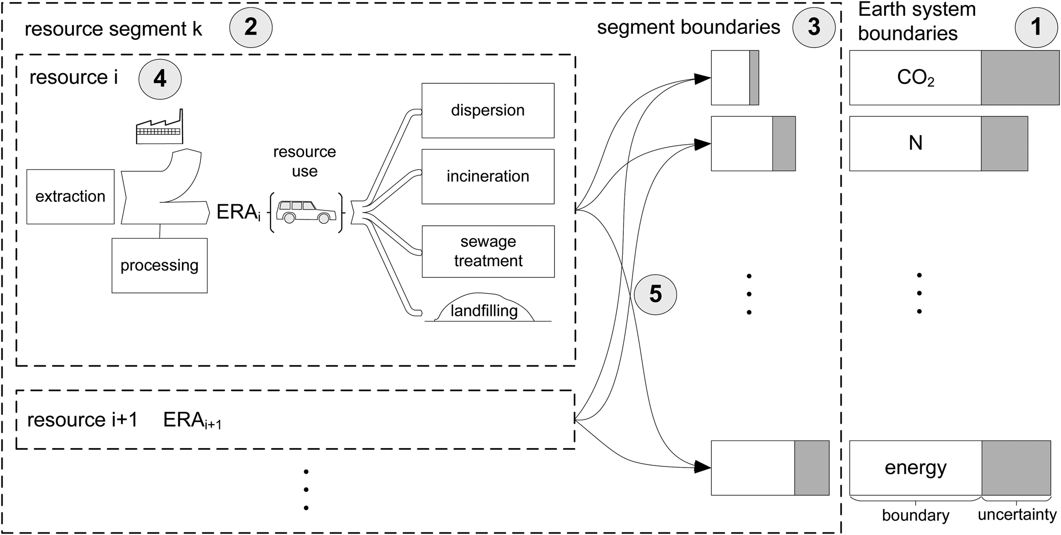
Fig. 1. Schematic representation of the ecological resource availability (ERA) method, consisting of five steps: (1) selection of Earth system boundaries; (2) resource segment definition; (3) allocation of safe operating space (e.g., by using environmentally extended input–output tables); (4) environmental impacts of resource production (e.g., by using life cycle assessment); and (5) upscaling of resource production until the impacts ‘hit’ the allocated segment boundaries to determine ERA.
In detail, the ERA method is composed of the following five steps (Figure 1):
(1) Selection of an environmental sustainability objective, relevant ESBs and a required level of confidence in the results.
(2) Choice of the resource or resource segment to be investigated. Selecting a resource segment requires the determination of the share of production (SoP) of different resources within the segment.
(3) Allocation of a share of the global boundaries to the segment.
(4) Calculation of the environmental impacts per unit of resource production and end-of-life (EoL) treatment (i.e., life cycle impacts excluding use phase).
(5) Scale-up of the combined resource production of the segment, until a first segment boundary is violated with the chosen probability of violation.
With these steps, the ERA is calculated as annual resource budgets for each resource within the segment. Each of the five steps is described in detail in the following subsections.
2.1. Selection of Earth system boundaries
The first step in the ERA method is to select an environmental sustainability objective and a set of suitable boundaries describing the objective. The boundaries can be global or regional, interdependent or independent, and be either driver, pressure, state or impact in the DPSIR frameworkFootnote 1 (Niemeijer & de Groot, Reference Niemeijer and de Groot2006, Reference Niemeijer and de Groot2008). The condition for selecting a boundary is that it needs to be measurable using the methods chosen to allocate the safe operating space (SOS; step 3) and quantify the impacts (step 4). In general, each boundary demarcates the maximum value for an indicator that can be tolerated by the Earth system before it collapses or changes irreversibly (Catton, Reference Catton1986; Rees, Reference Rees1996). The uncertainty range of the boundary can reflect the parameter uncertainty and/or increased risk to society associated with the transgression of the boundary value (Steffen et al., Reference Steffen, Richardson, Rockstrom, Cornell, Fetzer, Bennett and Sorlin2015).
The ERA method is based on the precautionary principle, which means that despite the often large uncertainties in both boundary values and impact measurements, the resulting ERA budgets needs to be viable with high confidence (Desing et al., Reference Desing, Widmer, Beloin-Saint-Pierre, Hischier and Wäger2019, Reference Desing, Brunner, Takacs, Nahrath, Frankenberger and Hischier2020). Therefore, an acceptable probability of violating the defined boundaries P v is required as an input parameter. This value is a normative choice, reflecting the acceptance of risk in society.
For the ERA calculations, the boundary values are stored in a three-dimensional matrix (n ESB × 1 × n runs), with the third dimension containing random values for each element in the other two dimensions according to the probability distribution of the respective boundary.
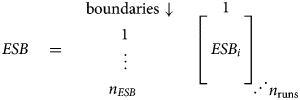 $$\eqalign{& ESB\quad = \quad \matrix{ {\vskip-5pt {\rm boundaries}\downarrow } \cr \matrix{\hskip -1.5pt{\displaystyle 1} \hfill \cr \vdots \hfill \cr \hskip -9pt n_{ESB} \hfill} \cr } \quad \mathop {\left[{\matrix{ {} \cr {ESB_i} \cr {} \cr } } \right]}\limits^ {\displaystyle 1} \matrix{ {} \cr {} \cr {} \cr {\vskip4pt\hskip-6pt{\mathinner{\mkern2mu\raise1pt\hbox{.}\mkern2mu \raise4pt\hbox{.}\mkern2mu\raise7pt\hbox{.}\mkern1mu}} n_{{\rm runs}}} \cr }} $$
2.2. Resource segment definition
The second step in the ERA method is to select the resource segment k to be investigated. Such a segment comprises one or several resources (e.g., metals). This choice may be limited depending on the data source used for allocation. For example, the Exiobase database (Stadler et al., Reference Stadler, Wood, Bulavskaya, Södersten, Simas, Schmidt and Tukker2018; Tukker et al., Reference Tukker, Poliakov, Heijungs, Hawkins, Neuwahl, Rueda-Cantuche and Bouwmeester2009) provides information on the aggregated industry level (e.g., casting of metals). In this case, the resource segment needs to comprise at least all (bulk) metals. When a resource segment comprises more than one resource, the relative SoP of each resource needs to be specified. The SoP expresses the fraction that a single resource contributes to the total mass flow of the segment. The SoP data are stored in a vector (n resources × 1).
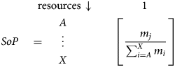 $$\eqalignb{& \matrix{ {\quad \quad \quad {\rm resources}{\mkern 1mu} \downarrow } \cr } \matrix{ {\quad \quad \,\,\,\,\,\,\quad 1} \cr } \cr & SoP\quad = \quad \matrix{ A \cr \vdots \cr X \cr } \quad \quad \quad \quad \left[{\matrix{ {} \cr {\displaystyle{{m_j} \over {\sum\nolimits_{i = A}^X {m_i} }}} \cr {} \cr } } \right]} $$
2.3. Allocation of safe operating space
The ESBs define the SOS (Rockström et al., Reference Rockström, Steffen, Noone, Persson, Chapin, Lambin and Foley2009a), within which collective human activities can be considered environmentally sustainable. This space needs to be allocated to specific activities in order to set boundaries for those activities. In the ERA method, the ESBs are allocated to the resource segment under investigation, resulting in segment boundaries SB k. This allocation is performed by assigning a share of the safe operating space (SoSOS) (Ryberg et al., Reference Ryberg, Owsianiak, Richardson and Hauschild2018b) to the segment k for each boundary i. There are many different possibilities to define the SoSOS (EEA & FOEN, 2020) (e.g., economic value of a resource – Ryberg et al., Reference Ryberg, Owsianiak, Clavreul, Mueller, Sim, King and Hauschild2018a, 2018b; grandfathering approach – Hollberg et al., Reference Hollberg, Lützkendorf and Habert2019; or future emission scenarios – Pineda et al., Reference Pineda, Tornay, Huusko, Delgado Luna, Aden, Labutong and Faria2015). In general, any allocation principle can be applied in the ERA method.
The allocated segment boundary (SB k), which is the absolute share of the total boundary available for the respective resource segment, is calculated by multiplying the diagonal of SoSOS with ESB for each Monte Carlo simulation run (third dimension). It has the same matrix dimension as ESB.
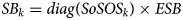 $$SB_k = diag\lpar {SoSOS_k} \rpar \times ESB$$
2.4. Environmental impacts of resource production
After specifying the segment boundaries, the impacts on these boundaries need to be determined for one unit of resource provision. Impacts not only arise from extraction and primary material production, but also from EoL treatment. Every material introduced into the socioeconomic system eventually finds its way back to the environment, be it through unintentional dispersion (e.g., abrasion) or intentional discharge (e.g., landfill) (Desing et al., Reference Desing, Brunner, Takacs, Nahrath, Frankenberger and Hischier2020). Following the responsibility principle,Footnote 2 environmental impacts for final disposal have to be added to primary production. Impacts associated with the use of the material, such as product manufacturing, product use and cycling strategies, are not considered in the ERA method, as these are covered in the respective sectors in the economy. Impacts resulting from the input of energy and materials in the use phase of the material are considered in the respective ERA budgets. Direct use impacts are to be considered in the relevant segments. Similarly, secondary material production can be considered as a separate segment with its own boundary, and thus it is assumed not to affect the ERA of primary materials. Cycling strategies do increase the resource base available to the economy, but only delay and do not prevent materials from entering final sinks.
Four principal disposal options can be distinguished: open dump (= dispersion), landfilling, incineration and sewage sludge. If the disposal routes are known (e.g., for plastics in Switzerland, see Kawecki & Nowack Reference Kawecki and Nowack2019), an overall waste process can be created as a combination of the four options. Otherwise, impacts can be modelled with an uncertainty range spanning the best and worst option.
The application of the precautionary approach necessitates modelling of uncertainties for unit impacts. For example, uncertainties in life cycle assessment (LCA) stem from the inventory uncertainties (e.g., measurement errors, spatial and temporal variability; Ecoinvent, 2013; Muller et al., Reference Muller, Lesage, Ciroth, Mutel, Weidema and Samson2014) and different life cycle impact assessment methods (e.g., different time horizons for global warming potentials). Data for unit impacts (UI) are stored in a three-dimensional matrix (n resources × n ESB × n runs):
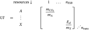 $$\eqalignb{& \matrix{ {\quad \quad \quad {\rm resources} {\mkern 1mu} \! \downarrow } \cr } \matrix{ {\quad \,\,\,\,\,\,\quad \ 1\ \quad \ldots\quad n_{ESB}} \cr } \cr & UI\quad = \quad \matrix{ A \cr \vdots \cr X \cr } \quad \quad \quad \quad \left[{\matrix{ {\displaystyle{\vskip10pt{m_{CO_2}} \over {m_A}}} \,\,\,\quad \,\,\,\,\,\,\quad \cr {}{}{} \cr\,\,\,\,\,\,\,\,\,\,\,\,\,\,\,\,\,\,\,\,\,\,\,\,\,\,\,\,\,\,\,\, {}{}{\displaystyle{{E_{el}} \over {m_X}}} \cr } } \right]}\matrix{ {} \cr {} \cr {}\cr {} \cr {{\mathinner{\mkern2mu\raise1pt\hbox{.}\mkern2mu \raise4pt\hbox{.}\mkern2mu\raise7pt\hbox{.}\mkern1mu}} n_{{\rm runs}}} \cr } $$
As a consequence of the global scope of the ERA method, the processes modelled to calculate the unit impacts have to be representative of the global average for primary production (e.g., global datasets in ecoinvent). Attention has to be paid to ensure that secondary materials are not included in these global averages.
2.5. Upscaling of resource production
The last step of the ERA method increases the production of a resource (and thus its environmental impacts) until the probability density functions (PDFs) of both the boundaries and environmental impacts overlap. As long as all possible impacts are smaller than all possible boundary thresholds, the system can be considered fully sustainable. However, as soon as some possible impacts are larger than some possible boundaries (i.e., when two PDFs start to overlap), there is an increasing probability that the system will violate the environmental sustainability criterion and thus be not sustainable (see Figure 2). If all impacts are larger than their respective boundaries, then the system is certainly not sustainable.
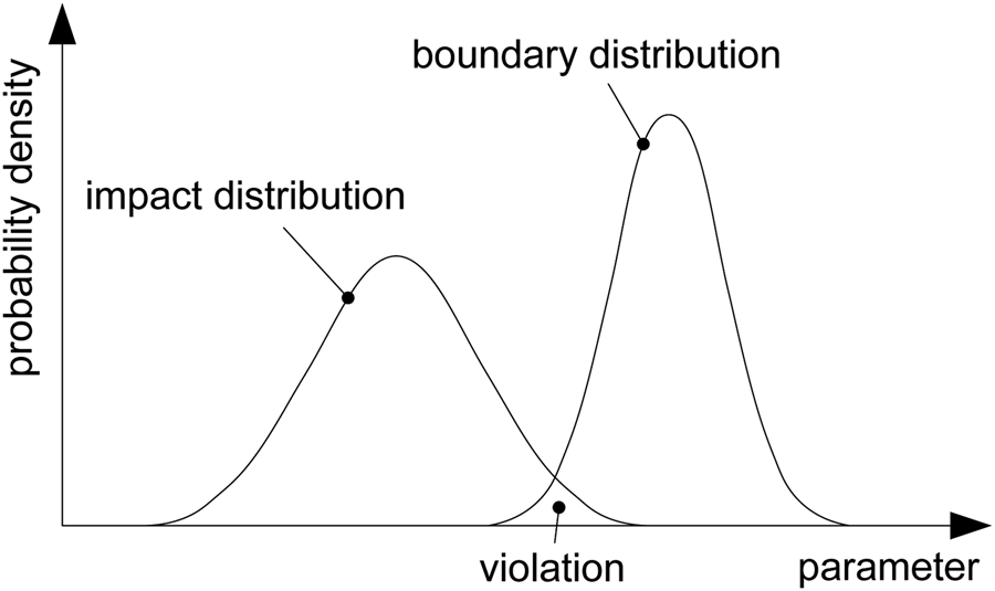
Fig. 2. Schematic representation of the concept of probability of boundary violation, which results from the overlap from the probability distribution of the environmental impacts with the distribution of the respective boundary.
The UI of the individual resources within one segment are combined to an overall unit impact for the segment, UI k (i.e., the impact caused by the production of one unit of the resource mix as specified by the SoP; see Section 2.2).
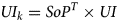 $$UI_k = SoP^T \times UI$$
The production volume of the resource mix in the segment ERA k is then increased stepwise, until one segment boundary SB is violated with the chosen probability of violation P v. As the calculation of P v,i in each step depends on the shape of the distributions of both impacts and boundaries, a numerical approach is taken. The initial ERA k,i is calculated as the  $1-{{P_v} \over 2}$-quantile of the UI k PDF and the ${{P_v} \over 2}$-quantile of the SB k PDF. In an iteration loop, the P v is calculated and the ERA k,i+1 increased or decreased until P v,i equals the required value P v.
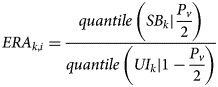 $$ERA_{k\comma i} = \displaystyle{{quantile\,\left({SB_k{\rm \vert }\displaystyle{{P_v} \over 2}} \right)} \over {quantile\,\left({UI_k{\rm \vert }1-\displaystyle{{P_v} \over 2}} \right)}}$$
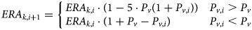 $$ERA_{k\comma i + 1} = \left\{{\matrix{ {ERA_{k\comma i}\cdot \lpar {1-5\cdot P_v\lpar {1 + P_{v\comma i}} \rpar } \rpar } \hfill & {P_{v\comma i} \gt P_v} \hfill \cr {ERA_{k\comma i}\cdot \lpar {1 + P_v-P_{v\comma i}} \rpar } \hfill & {P_{v\comma i} \lt P_v} \hfill \cr } } \right.$$
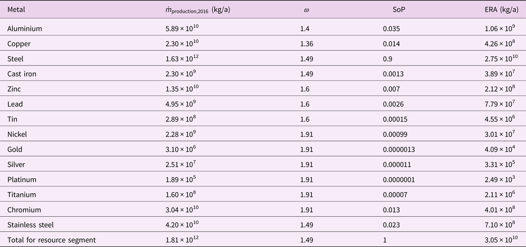
The resource budget ERA k is calculated for each boundary separately. As all SBs need to be respected, the smallest ERA k defines the budget for the resource segment. For each resource in the resource segment k, the resource budget is calculated through multiplying the smallest ERA k with the SoP. ERA is a vector (n resources × 1) and contains the ERA budget for each of the resources in the segment with the chosen confidence 1 − P v.
 $$ERA = SoP\cdot min\lpar {ERA_k} \rpar $$
3. Case study: metals
In the following subsections, we demonstrate the application of the ERA method for the resource segment metals, using a grandfathering allocation approach.
3.1. Selection of Earth system boundaries: adaptation of planetary boundaries
As the sustainability objective, we choose the protection of the Holocene-like state of the Earth system and use the PB framework as a set of ESBs (Rockström et al., Reference Rockström, Steffen, Noone, Persson, Chapin, Lambin and Foley2009b; Steffen et al., Reference Steffen, Richardson, Rockstrom, Cornell, Fetzer, Bennett and Sorlin2015). The adaptation of the boundaries is based on the literature and for the purpose of demonstrating the ERA method. Furthermore, the probability of violating the boundaries is set to P v = 0.01 (Desing et al., Reference Desing, Widmer, Beloin-Saint-Pierre, Hischier and Wäger2019) to illustrate the method. This is in between the probability of failure tolerated for critical technical systems (usually <0.001; see Table S2) and deemed acceptable in current Earth system governance (e.g., P v = 0.33 for reaching the 2.0°C target (IPCC, 2013); P v = 0.5 for reaching the 1.5°C target (IPCC, 2018), despite potentially catastrophic effects (Lenton et al., Reference Lenton, Rockstrom, Gaffney, Rahmstorf, Richardson, Steffen and Schellnhuber2019)).
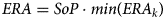
The PBs define boundary values for nine crucial Earth system processes.Footnote 3 When crossing the boundary values, fast and irreversible environmental change is expected to happen, leading to a new Earth system state being less hospitable for human civilizations and most other forms of life (Steffen et al., Reference Steffen, Rockstrom, Richardson, Lenton, Folke, Liverman and Schellnhuber2018). Respecting the PBs can be seen as necessary for reaching environmental sustainability, but not sufficient to ensure it (Chandrakumar & McLaren, Reference Chandrakumar and McLaren2018). The PB framework can be refined with more detailed control variable definitions (e.g., for biodiversity, see Alig et al., Reference Alig, Frischknecht, Nathani, Hellmüller and Stolz2019; Mace et al., Reference Mace, Reyers, Alkemade, Biggs, Chapin, Cornell and Woodward2014) or extended to other variables (e.g., net primary production O'Neill et al., Reference O'Neill, Fanning, Lamb and Steinberger2018; Running, Reference Running2012). To show this, we add a boundary on renewable energy potentials (Desing et al., Reference Desing, Widmer, Beloin-Saint-Pierre, Hischier and Wäger2019), representing the amount of energy that can be appropriated by society without transgressing other critical PBs (e.g., land-system change) or compromising food supply. The global appropriable technical potential (ATP) for renewable energy is estimated to be  $ATP_{el\comma p = 0.98} = \lpar {1.52_{{-}0.81}^{ + 1.24} } \rpar \times 10^{14}{\rm W}$ (Desing et al., Reference Desing, Widmer, Beloin-Saint-Pierre, Hischier and Wäger2019). This added boundary is a global boundary for a driver of environmental pressure and is particularly relevant for a CE, as for increasingly closed material cycles, energy may become limiting (Ayres, Reference Ayres1999).
The PBs themselves need translation in order to be compatible with the measurement of impacts with units commonly used in LCA and environmentally extended input–output tables (EE-IOTs). This has been addressed by various authors using different approaches (e.g., impact reduction targets in LCA – Sandin et al., Reference Sandin, Peters and Svanström2015; deriving measurable boundaries – Dao et al., Reference Dao, Peduzzi, Chatenoux, De Bono, Schwarzer and Friot2015, Reference Dao, Peduzzi and Friot2018; Meyer & Newman, Reference Meyer and Newman2018; boundary characterization factors – Ryberg et al., Reference Ryberg, Owsianiak, Richardson and Hauschild2018b; per-capita impact allowance – Bjørn & Hauschild, Reference Bjørn and Hauschild2015; Doka, Reference Doka2016; combining footprints with PBs – Fang et al., Reference Fang, Heijungs and De Snoo2015). For the purpose of illustrating the method, we do not consolidate the various different approaches, which is a topic for further research. Meanwhile, we derive measurable boundaries and uncertainty ranges by using a combination of approaches in the literature (Table 1, Figure S1 and SM), except for the three boundaries described in the following. We adopt the biodiversity boundary from Doka (Reference Doka2016); however, we highlight the need to refine this boundary in the future. For example, up-to-date and United Nations Environment Programme (UNEP)–Society of Environmental Toxicology and Chemistry (SETAC) recommended methods to assess the global fraction of species loss exist (UNEP & SETAC, 2016) and can be converted into extinction rates (Alig et al., Reference Alig, Frischknecht, Nathani, Hellmüller and Stolz2019). The land appropriation boundary in Ryberg et al. (Reference Ryberg, Owsianiak, Richardson and Hauschild2018b) only considers forest area, which cannot be measured easily with LCA and EE-IOTs, whereas in Doka (Reference Doka2016), all biomes other than forest can be appropriated, endangering biodiversity in these biomes. Bjørn and Hauschild (Reference Bjørn and Hauschild2015) define the land boundary based on minimum biodiversity conservation targets; however, they do not consider the forest boundary set with climate considerations of the original PBs. We therefore adopt the land boundary setting in our earlier work (Desing et al., Reference Desing, Widmer, Beloin-Saint-Pierre, Hischier and Wäger2019), which combines the remaining forest area boundary from Steffen et al. (Reference Steffen, Richardson, Rockstrom, Cornell, Fetzer, Bennett and Sorlin2015) with the ‘Nature Needs Half’ proposal (Dinerstein et al., Reference Dinerstein, Olson, Joshi, Vynne, Burgess, Wikramanayake and Saleem2017) for all other biomes.
Table 1. Translation of Earth system boundaries considered in this study (10 variables from the planetary boundaries framework (Rockström et al., Reference Rockström, Steffen, Noone, Persson, Chapin, Lambin and Foley2009b; Steffen et al., Reference Steffen, Richardson, Rockstrom, Cornell, Fetzer, Bennett and Sorlin2015) and complemented by the appropriable technical potential for renewable energy (Desing et al., Reference Desing, Widmer, Beloin-Saint-Pierre, Hischier and Wäger2019)) to annual flows compatible with environmentally extended input–output tables and life cycle assessment units. Intervals are expressed in this paper in their mathematical form (i.e., x = [x min, x max) meaning x min ≤ x < x max). This notation implies a level of confidence of the interval of p = 1. Uncertainty of values is reported for a specified level of confidence of the interval p, the 50% value and the lower and upper deviations that confine the interval.
For the CO2 boundary, we propose a different approach to be in line with the ERA method's scope of maintaining a sustainable state of the Earth system over time. The atmospheric CO2 concentration needs to be constant at or below the PB. Without human influence, the CO2 concentration in the atmosphere had been decreasing (Foster et al., Reference Foster, Royer and Lunt2017). Continuous CO2 emissions are possible to the extent of continuous removal by natural processes. CO2 removal by sedimentation and weathering has been relatively constant over the last 20 Ma (IPCC, 2013; Stein, Reference Stein1991), when atmospheric CO2 concentration had been below 450 ppm (IPCC, 2013) and therefore within or below the PB, and so overcompensating for natural CO2 release (e.g., volcanism). The condition of keeping the concentration constant allows continuous (but small) emissions of anthropogenic CO2 of  $\dot{m}_{{\rm C}{\rm O}_2} \lt [ {8.25\comma \;22} ] \times 10^{11}\,{{{\rm kg}} / {\rm a}}$. This boundary translation is in contrast to other studies, where the CO2 emission boundary is set with a specific time horizon (e.g., 300 a – Ryberg et al., Reference Ryberg, Owsianiak, Richardson and Hauschild2018b; or for negative emissions required between 2050 and 2080 to reach the 350 ppm target before 2100, see Meyer & Newman, Reference Meyer and Newman2018).
3.2. Resource segment definition: metals
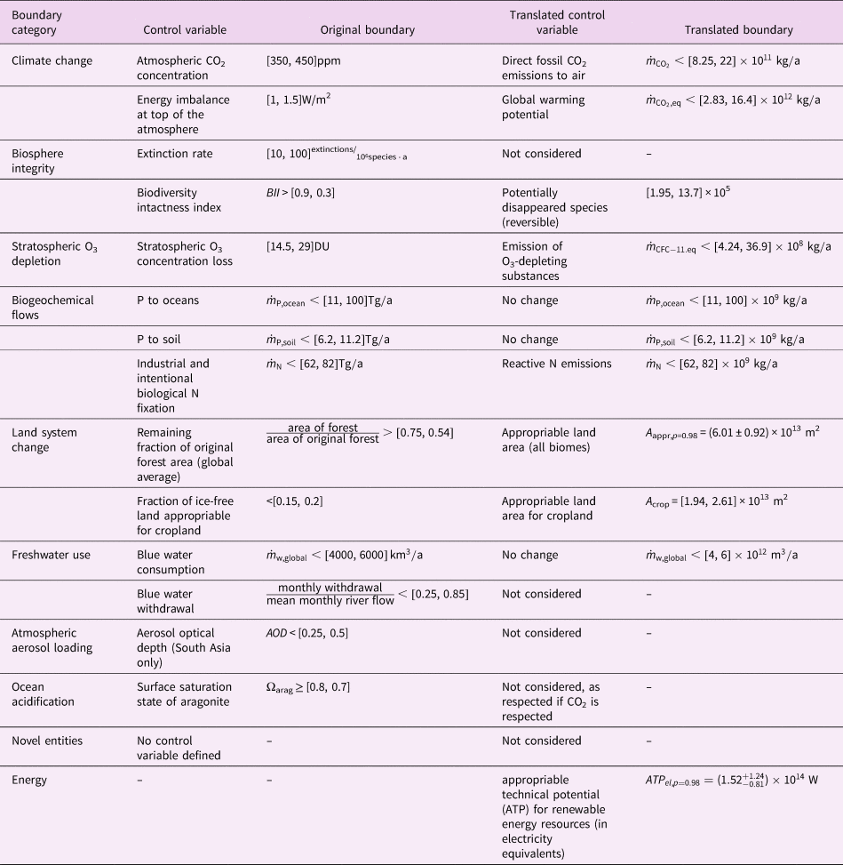
The resource segment metals includes all 14 metals given in the Exiobase database: aluminium, copper, steel, cast iron, zinc, lead, tin, nickel, gold, silver, platinum, titanium, chromium and stainless steel. Other metals (e.g., rare earth metals) are not included in this segment. The production share (mass fraction) of all materials within the segment (SoP) needs to be defined. We use production data from USGS (2016) and for cast iron from Ashby (Reference Ashby2012), as this material is not reported in the first source. In order to calculate the SoP as the final output of resource segments to the rest of the economy without double counting the production that is necessary to produce other materials, the production data need to be corrected to production output with the oversize factor  $\omega = {{{\dot{m}}_{{\rm overall}\;{\rm production}}} \over {{\dot{m}}_{{\rm production}\;{\rm output}}}}$ (Cabernard et al., Reference Cabernard, Pfister and Hellweg2019; Dente et al., Reference Dente, Aoki-Suzuki, Tanaka and Hashimoto2018; see Table 2 and SM Section 3.4).
Table 2. Global production in 2016  $\dot{m}_{{\rm production}\comma 2016}$ (USGS, 2016), oversize factor ω, share of production (SoP) and ecological resource availability (ERA) for the investigated metals.
3.3. Allocation of the safe operating space: grandfathering approach
The allocation principle has an important influence on the results (Bjørn et al., Reference Bjørn, Richardson and Hauschild2018; Ryberg et al., Reference Ryberg, Owsianiak, Clavreul, Mueller, Sim, King and Hauschild2018a; Sabag-Munoz & Gladek, Reference Sabag-Munoz and Gladek2017). To illustrate the ERA method, a grandfathering allocation approach (Sabag-Munoz & Gladek, Reference Sabag-Munoz and Gladek2017) is applied in this case study, where each resource receives a SoSOS equal to its historic impact share. For example, if the production of steel is responsible for 9% of the global CO2 emissions today, steel receives the same share of the CO2 boundary. This approach reflects the question: what if we rescale today's socioeconomic system to fit within ESBs? As today's world economy already transgresses six boundaries (see Figure 3), resource production as well as final demand would have to be downscaled significantly, leaving large parts of the global society without access to basic services. This scenario is therefore to be seen as indicative only.
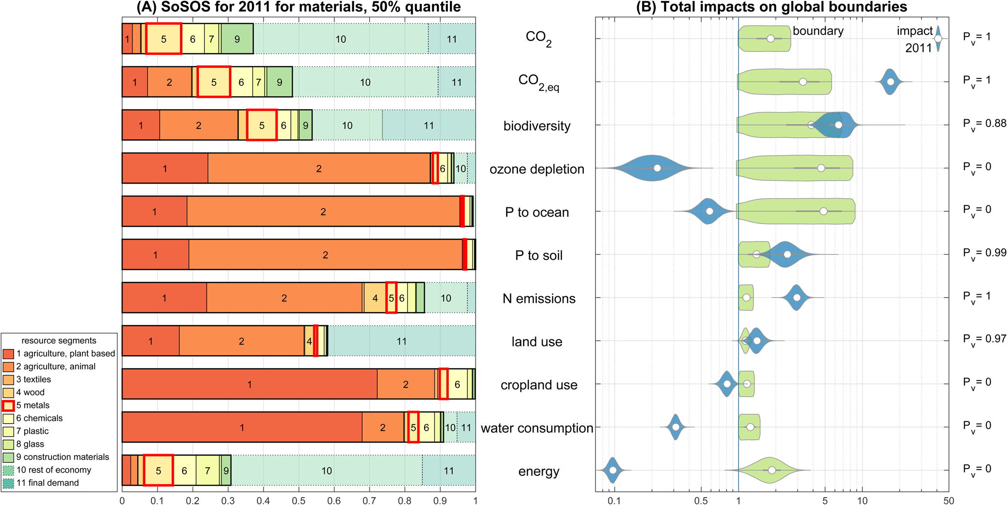
Fig. 3. Panel (A) shows the relative impact contribution for nine resource segments (including supply chain impacts), which defines the share of the safe operating space (SoSOS) in the grandfathering approach. The contributions of the resource segment metals (5) are highlighted with red boxes. The rest of economy segment (10) represents all activities that are not part of the resource production chain (e.g., manufacturing of end-user devices), while the final demand segment (11) comprises the purchase and use of goods and services by the end consumer. In panel (B), the total global environmental impacts of the socioeconomic system in the year 2011 is compared to the global boundaries. Six out of the 11 boundaries are crossed with a probability greater than 1%. All values are scaled relative to the 0.5 percentile of the respective boundary distribution ( $1\hat{ = }ESB_{p = 0.005}$).
The calculation of the relative historic impact of each resource segment is conducted with a top-down approach, using the Exiobase database v3.4 (Stadler et al., Reference Stadler, Wood, Bulavskaya, Södersten, Simas, Schmidt and Tukker2018; Tukker et al., Reference Tukker, Poliakov, Heijungs, Hawkins, Neuwahl, Rueda-Cantuche and Bouwmeester2009).Footnote 4 In Exiobase, the emissions for each industry are reported that are directly produced through the industry's activity itself. Industries concerned with the production or EoL treatment of materials are grouped into nine resource segments, and the remaining industries are aggregated into rest of economy. Impacts associated with consumption in households are contained in the final demand category. We use the approach from Cabernard et al. (Reference Cabernard, Pfister and Hellweg2019) to calculate the cumulative impacts for nine resource segments without double counting the impacts already included in the supply chain of another segment (e.g., metals necessary to produce plastics). A detailed description of the calculation, the impact characterization methods used and the uncertainty modelling can be found in the SM. The results of the SoSOS calculations are shown in Figure 3(A). The SoSOS is determined by the 50% value of the uncertainty distribution resulting from the Monte Carlo simulation. This set of values is chosen so that the total relative impacts add up to 1 and the full SOS can be utilized. The SoSOS has been determined with data from the year 2011 (the difference from the same procedure with data from 1995 is small, Person covariance r = 0.9954). The overall impact for the year 2011 on the global boundaries as calculated with Exiobase is qualitatively consistent with Steffen et al. (Reference Steffen, Richardson, Rockstrom, Cornell, Fetzer, Bennett and Sorlin2015), except for the two climate boundaries. In Steffen et al. (Reference Steffen, Richardson, Rockstrom, Cornell, Fetzer, Bennett and Sorlin2015), the impact on these boundaries is within the uncertainty range, whereas in our assessment, they exceed the boundaries by far (see Figure 3(B)). This is due to the translation of state variables (CO2 concentration, irradiation imbalance) into pressure variables ( $\dot{m}_{{\rm C}{\rm O}_2}$, $\dot{m}_{{\rm C}{\rm O}_2\comma {\rm eq}}$; see Section 3.1).
3.4. Environmental impacts of metals production
The impacts on the selected boundaries caused by the production and EoL treatment of one unit of material are calculated with a bottom-up approach using LCA and ecoinvent v3.5 (Wernet et al., Reference Wernet, Bauer, Steubing, Reinhard, Moreno-Ruiz and Weidema2016). This database is chosen because it aims to offer global coverage of the supply chains of materials in necessary detail. Hence, for each material, at least a global average dataset is available as required in the ERA method for calculating global resource budgets. The unit impacts are constructed from two processes: (1) primary material production (e.g., aluminium, primary, ingot); and (2) EoL treatment, which can consist of several processes (e.g., incineration, landfill). From ecoinvent, the cut-off (or recycled content) system model is chosen, as in this model the primary material production chains show the entire impacts of the production steps; no parts of these impacts are already allocated to secondary material cycles or to EoL treatment processes. At the same time, the EoL processes contain only the impacts related to the respective treatment processes. An overview of all of the processes considered and the impact characterization methods and uncertainty considerations for this analysis is provided in the SM.
3.5. Upscaling of resource production: ERA determination
Following the calculation steps (Section 2.5) and using n runs = 105 simulation runs leads to the results as depicted in Figure 4. The limiting SB for metals is CO2 due to the large overshoot of global impacts on this boundary. The production in 2016 (USGS, 2016), ω, SoP and ERA budgets are given in Table 2 for the metal segment. The ERA for the whole segment is 3.5 × 10¹⁰ kg/a and thus is 40 times smaller than production output in the year 2016. In other words, the primary resource production must be reduced by a factor of 40 to be within the selected ESBs in the grandfathering approach. The CO2 boundary is limiting the production of metals (see Figure 4), as it is the boundary that is crossed the most on the global scale (see Figure 3). Within the segment, steel is dominating the impact shares due to its large production share (SoP steel = 0.9). The depletion time of extractable global resources (Henckens et al., Reference Henckens, Driessen and Worrell2014; USGS, 2016) at the rate of ERA is for all investigated metals >>1500 a (except 920 a for gold). This confirms the hypothesis that the depletion of physical resources is not the pressing constraint for a sustainable economy, but rather the environmental impacts caused.
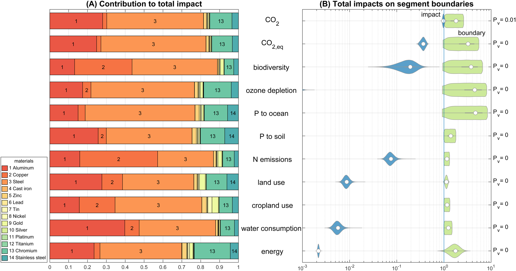
Fig. 4. Panel (A) shows the relative contribution of each metal to the total environmental impacts of the resource segment metals. In panel (B), the cumulative impacts of metals (blue) are compared relative to the 0.5 percentile of the allocated boundary for the metal segment (green) ( $1\hat{ = }SB_{p = 0.005}$). CO2 is limiting the metal segment ( $P_{v\comma {\rm C}{\rm O}_2} = 0.01$).
4. Discussion
Based on our settings above, we show that ERA budgets for metals are 40 times smaller than production rates in 2016, assuming state-of-the-art-technology, today's resource demand pattern (grandfathering allocation) and current production shares in the metal sector. The CO2 boundary is thereby limiting the ERA budget due to today's carbon-intensive production technology. The climate crisis is, according to our findings, the most pressing environmental concern, followed by biodiversity loss (see Figure 3(B)). This confirms the current societal and political focus on CO2. However, a shift in production technology (e.g., fossil-free) and towards less carbon-intensive materials (e.g., biomass) may lead to increased pressure on other boundaries.
The method proposed here is capable of avoiding hidden burden shifting among the included boundary categories, and additional categories can be included in the method to avoid negative effects on processes currently not considered (e.g., soil quality – Chandrakumar & McLaren, Reference Chandrakumar and McLaren2018; imperishable waste – Meyer & Newman, Reference Meyer and Newman2018). Furthermore, the flexible design of the ERA method allows us to consider different technologies for resource production, allocation principles or sustainability objectives and thus can serve as a scenario tool for modellers. The method can also be used to evaluate, for example, a fossil-free scenario, where resource production processes do not run on fossil fuels, but on renewable energy exclusively. In this way, the ERA method can be used as a quantitative tool to evaluate the effects of different scenarios on the sustainable consumption scale of resources for the future. Such scenarios can form the basis for sustainable resource governance and the design of effective policies. For example, the ERA method can be used to evaluate different policy options (e.g., allocation principles, technology promotion) in terms of their effects on the availability of resources to society. Resource budgets can serve governments and international organizations as a strategic prioritization tool for resource governance. Furthermore, the ERA budgets can be used for decision support, such as material selection for product design or assessment of products’ and companies’ resource footprints (Desing et al., Reference Desing, Braun and Hischiersubmitted). The concept of a resource budget allows us to include ESBs in decision-making, similarly to today's consideration of financial budgets.
For the moment, the ERA method is designed to calculate global budgets only. However, environmental circumstances on a regional level may be different compared to the global average (e.g., biodiversity – Chaudhary et al., Reference Chaudhary, Pfister and Hellweg2016; land use – Gerten et al., Reference Gerten, Heck, Jägermeyr, Bodirsky, Fetzer, Jalava and Schellnhuber2020; water scarcity –Gleeson et al., Reference Gleeson, Wang-Erlandsson, Zipper, Porkka, Jaramillo, Gerten and Famiglietti2020; Pfister & Bayer, Reference Pfister and Bayer2014; Zipper et al., Reference Zipper, Jaramillo, Wang-Erlandsson, Cornell, Gleeson, Porkka and Gordon2020) and therefore require regionalization. In principle, integrating regionalized boundaries is possible in the ERA method; however, this requires both the setting of regional boundaries as well as regionalized impact assessment.
Another limitation is the allocation process of the boundary to resource segments. In this paper, we applied a grandfathering allocation approach to divide the SOS based on historic emission shares for the purpose of demonstration. While informative, we do not consider this a realistic allocation principle, as scaling the whole economy equally will result in an economy that is unable to provide a decent living standard (Rao & Min, Reference Rao and Min2018) for a growing global population (UN Department of Economic and Social Affairs, 2019). For example, food production will be downscaled by the same order of magnitude as metals, which may lead to starvation. Therefore, it is essential to define allocation principles that allow a decent life for a prospective global population of  $N_{p = 0.95} = \lpar {10.87_{{-}1.45}^{ + 1.79} } \rpar \times 10^9$ in 2100 (UN Department of Economic and Social Affairs, 2019). For example, an allocation approach that assigns very small shares to fossil resources (coal, oil, gas) would free up operating space for other resources and increase their budgets. Even more interesting for the transformation towards a sustainable economy would be to develop an allocation principle that increases the final services provided for society (e.g., based on Science Based Targets (Pineda et al., Reference Pineda, Tornay, Huusko, Delgado Luna, Aden, Labutong and Faria2015), which try to define ambitious but realistic emission reduction scenarios for different industries in a participatory approach). This is not considered in this proof of concept of the ERA method in this paper, but it represents a potential area for further research. For the application of the ERA method, it must always be made clear which allocations and assumptions have been chosen.
5. Conclusion and outlook
In this paper, we presented a novel method – the ERA method – to calculate the maximum production of primary materials that respects ESBs. The ERA method effectively translates ESBs into annual primary material production budgets and thus brings absolute environmental limits one step closer to decision-makers. Materials bring benefits to society; therefore, they are at the core of decision-making on different levels (e.g., product design, resource governance) – in contrast to environmental impacts.
We have shown in the exemplary application of the ERA method for metals that current production rates will deplete the sustainably available budgets on 9 January (in analogy to Earth Overshoot DayFootnote 5) if we continue to produce them with current technology, today's economic structure and current production shares in the metal sector. This confirms our hypothesis that environmental impacts are presently the most limiting factor for sustainable metals production. But how can we avoid running out of sustainably produced metals? The ERA method can help to evaluate the effectiveness of various measures, for example:
• Reducing the primary resource intensity of the economy through resource efficiency and increased material cycling;
• Shifting technology to low carbon intensity (e.g., renewable energy – Desing et al., Reference Desing, Widmer, Beloin-Saint-Pierre, Hischier and Wäger2019; International Energy Agency, 2019; Pineda et al., Reference Pineda, Tornay, Huusko, Delgado Luna, Aden, Labutong and Faria2015; or direct hydrogen reduced steel – Ahman et al., Reference Ahman, Olsson, Vogl, Nykvist, Maltais, Nilsson and Nilsson2018);
• Optimizing the SoP by using more resources with low unit impacts. This is, however, only possible to a certain extent, as every resource has specific properties required in its applications (e.g., electrical conductivity of copper).
Applying the ERA method allows us to evaluate how effective these options are at increasing the resource budgets for society, and thus it provides companies and governments with ‘consistent and accurate feedback about whether the magnitude of their impacts mitigation efforts is sufficient to halt large scale planetary change’ (Sabag-Munoz & Gladek, Reference Sabag-Munoz and Gladek2017, p. 5).
Supplementary materials
The supplementary text contains details on uncertainty modelling, planetary boundaries translation, allocation of safe operating space to industrial sectors using Exiobase, resource impact calculation using ecoinvent, a glossary and a list of abbreviations used in the article. Furthermore, the calculation data and Matlab (R2018) code files can be accessed here: https://doi.org/10.5281/zenodo.3629366.
The supplementary material for this article can be found at https://doi.org/10.1017/sus.2020.26.
Acknowledgements
The authors thank L. Cabernard (ETH) for assistance with Exiobase and P. Wager (Empa), S. Hellweg (ETH) and two anonymous reviewers for useful comments on the manuscript.
Author contributions
HD conceived and designed the method; HD wrote the software; HD and GB gathered and analysed data and performed the case study; HD, GB and RH wrote the paper; RH supervised HD and GB; RH acquired funding and administrated the project.
Financial support
This research is part of the project ‘Laboratory for Applied Circular Economy’, funded by the Swiss National Science Foundation grant number 407340_172471 as part of the National Research Program ‘Sustainable Economy: resource-friendly, future-oriented, innovative’ (NRP 73).
Conflict of interest
The authors declare no conflict of interest.
Ethical standards
Both the paper and the supplementary materials are the original work of the authors.


 Open access