


1 Introduction
Studies of Arctic sea-ice variability on the interannual and decadal scales have heretofore been based almost exclusively on statistical or empirical analyses of observational data (e.g. Reference SandersonSanderson 1975, Reference KellyKelly 1978, Reference RogersRogers 1978, Reference Walsh and JohnsonWalsh and Johnson 1979, Reference Lemke, Trinkl and HasselmannLemke and others 1980, Reference SmirnovSmirnov 1980). The statistical analyses are severely constrained by the observational data, which are limited to approximately 15 years of satellite-derived hemispheric coverage or to longer periods of irregular coverage for portions of the Arctic periphery. Moreover, the observational data are limited almost exclusively to areal ice extent. The data therefore do not permit analyses of climatically relevant variables such as ice thickness, horizontal heat and mass transports, and vertical heat fluxes.
Numerical modeling provides an alternative approach to the large-scale variability of sea ice. When driven by time-dependent fields of atmospheric data, dynamic-thermodynamic sea-ice models provide fields of ice concentration, thickness and velocity which permit the construction of mass budgets for various high-latitude regions. Relatively few model studies have addressed sea-ice fluctuations over time periods longer than several weeks. Monthly climatological temperature and pressure fields were used in a series of equilibrium simulations by Reference Parkinson and KelloggParkinson and Washington (1979) and Reference Parkinson and KelloggParkinson and Kellogg (1979). In the latter study, the sensitivity of the ice to a large-scale warming was examined by imposing spatially and temporally invariant increases of surface air temperature. A 5 K warming of this kind resulted in a complete disappearance of the Arctic ice during summer. Reference Manabe and StoufferManabe and Stouffer (1980) performed a series of multiyear simulations with a coupled ice-ocean-atmosphere model. Sea ice was represented as a motionless slab without leads in this experiment designed to address the sensitivity to a C02-induced warming. While the CO2 sensitivity was indeed partially attributable to sea-ice effects, it should be noted that the control experiment (present CO2) produced a winter ice cover that is approximately twice as extensive as observed in the Arctic but only half as extensive as observed in the Antarctic (Reference Manabe and StoufferManabe and Stouffer 1980: fig.11). In another coupled model simulation, Reference Washington, Semtner, Meehl, Knight and MayerWashington and others (1980) employed a simplified thermodynamic model in which ice growth and decay were determined from precipitation and/or flux imbalances. Sea-ice dynamics were not included. The discrepancies between the simulated and observed ice coverage included an excess of simulated ice in the North Atlantic during the non-summer months. In the central Arctic, the simulated ice thickness (~1.5 m) was considerably smaller than the values of 3 to 4 m deduced from submarine data (Reference LeSchack, Hibler and MorseLeSchack and others 1971).
Hibler (Reference Hibler1979, Reference Hibler1980) used observed forcing data from a single year to drive a dynamic-thermodynamic model in a series of periodic equilibrium simulations for the Arctic Basin. The same model was used by Reference Hibler and WalshHibler and Walsh (1982) in simulations of northern-hemisphere sea-ice fluctuations during the period 1973–75. The latter simulations yielded a seasonal cycle with excessive amounts of ice in the North Atlantic during winter and with somewhat excessive amounts of open water in the central Arctic during summer. Despite these seasonal biases, the simulated and observed interannual fluctuations were similar in magnitude and positively correlated. Considerable interannual variability was apparent in the three-year simulation. While these simulations established the feasibility of using a dynamic-thermnodynamic sea-ice model for studying sea-ice fluctuations, the conclusions were subject to uncertainties concerning (i) the representativeness of the three-year sample of fluctuations, and (ii) the impact of the model “spin-up” on the three-year results. The present work extends these earlier simulations to the decadal scale (20 years) and in-corporates several changes in the model thermodynamics (section 2). The objective of the work is an analysis of large-scale multiyear sea ice-fluctuations in the context of the mass budgets of various sectors of the high-latitude ocean. As noted earlier, such an analysis must rely heavily on model-generated fields of ice thickness, compactness and velocity.
2 Model Summary
The essential features of the model are (a) a momentum balance based on geostrophically-derived air and water stresses, Coriolis force, ocean tilt, internal ice stress and inertial terms, (b) an ice rheology based on a viscous-plastic constitutive law and an ice-strength parameter P*, (c) an ice-thickness distribution characterized by the compactness A and the mean ice thickness h averaged over an entire grid cell, (d) a thermodynamic code in which vertical growth rates are estimated from heat-budget computations at the top and bottom surfaces of the ice and from the heat stored in a motionless oceanic boundary layer. Details of the model formulation are given by Hibler (Reference Hibler1979, Reference Hibler1980). Except for the modifications described below, the present simulations were based on the same version of the model and spatial grid used by Reference Hibler and WalshHibler and Walsh (1982).
2(a) Model domain
The domain used by Reference Hibler and WalshHibler and Walsh (1982) has been expanded by ~ 600 km to include a larger portion of the Pacific sub-Arctic. The simulations are now performed on a 38 × 31 grid with a resolution of 222 km (Fig.1). While the use of a relatively coarse horizontal resolution is dictated by the availability of computer resources, simulations driven by periodic forcing on a 125 km grid covering the Arctic Basin (Reference HiblerHibler 1979) produced results which were quite compatible with those obtained for the same region in the present work.

Fig. 1 The model grid and numbered regions.
2(b) Explicit treatment of snow cover
In the previous simulations snow cover was parameterized only through the surface albedo, which was assigned a value corresponding to ice or snow when the air temperature was above or below freezing, respectively. Snow is now accumulated during the non-summer months according to the prescribed accumulation rates of Reference Parkinson and KelloggParkinson and Washington (1979). The thermal conductivity of the snow/ice layer is represented by a single value corresponding to a weighted sum of the conductivities of snow and ice; the weighting factors are the snow- and ice-fractions of the total thickness. When the air temperature is above freezing, the snow must melt completely before the ice thickness is reduced by surface melt. The prescribed surface albedos of snow and ice are 0.80 and 0.65, respectively.
2(c) Multilevel thermodynamic computations
Thermodynamic computations were previously performed for two levels: open water (h = 0) and an effective thickness heff, representing the mean thickness of ice in the ice-covered portion of the grid cell. In order to incorporate the strong thickness-dependence of ice-growth rates (e.g. Reference MaykutMaykut 1982), heff is replaced by a seven-level distribution of thicknesses equally spaced between 0 and 2heff. While a more realistic thickness distribution can be obtained from multilevel dynamic computations (e.g. Reference HiblerHibler 1980) using the ice-thickness distribution theory developed by Reference Thorndike, Rothrock, Maykut and ColonyThorndike and others (1975), the treatment used here is regarded as a first-order attempt to include a range of thicknesses in the model thermodynamics.
Under growth conditions the snow cover is similarly partitioned into a seven-level linear distribution of snow depths. This strategey is based on the assumption that thin (new) ice will generally be covered by less snow than will thick (old) ice. Under melt conditions, which generally occur in spring and summer after much of the snow has been subjected to considerable blowing and drifting, the snow is assumed to be uniformly distributed over the ice-covered portion of each grid cell. The snow distribution corresponding to melt conditions is imposed whenever the surface temperature exceeds 0°C at the surface of ice of thickness heff.
3 Meteorological Forcing Data
The model is run with a one-day timestep using observed atmospheric forcing data from the period 1961 to 1980, inclusive. Daily wind fields are computed geostrophically from the National Center for Atmospheric Research (NCAR) set of northern-hemisphere sea-level pressure analyses, which are in the form of 5 × 5° latitude-longitude grids. Conversion to the Cartesian coordinates of the ice model is accomplished by bilinear interpolation. A total of 7 300 daily pressure grids were required for the 20-year simulations.
Air temperature anomalies are obtained from the so-called “Russian surface temperature data set” (Reference VinnikovVinnikov 1977, Reference RobockRobock 1982), which contains monthly temperature anomalies for the northern hemisphere on a 5 × 10° latitude-longitude grid. These anomalies are added to the climatological monthly mean temperatures of Reference Crutcher and MeserveCrutcher and Meserve (1970) and interpolated bilinearly to the ice model grid. Daily temperatures are then computed by a cubic spline interpolation from the monthly values, which are assumed to correspond to the mid-points of the respective calendar months.
Because the Russian temperature tape available for this work ended with December 1976, monthly climatological mean temperatures were used for the final four years (1977–80). The monthly means were computed from the temperatures of the first 16 years (1961–76) of the simulation period.
The relative humidities required for the computation of the downcoming longwave radiation were assumed to be 90% at all times and grid points. Earlier tests based on the years 1973–75 had shown that the results were quite insensitive to this assumption.
Finally, the absence of snowfall data for the Arctic required the use of the climatological snow-accumulation rates described in section 2(b). The model sensitivity to interannual snowfall variations may indeed be considerable and will be investigated in the near future.
4 Results
The simulations were Initiated with thickness fields varying linearly from 0 at the lateral boundaries to 3 m at the center of the grid. A two-year “spin-up” using observational data for 1961–62 was then performed before the 1961–80 simulation. Earlier tests with data for 1973–75 (Reference Hibler and WalshHibler and Walsh 1982) showed that the simulated fields of thickness, drift and compactness were within 5% of periodic equilibrium by the third year of this type of spin-up. The model was therefore run for 22 years of simulation time, although the results from the two-year spin-up are not included in the following discussion.
Two simulations were performed in order to identify the effects of the model dynamics. In the first, hereafter denoted as simulation DT, both dynamics and thermodynamics were included. In the second, hereafter denoted as simulation T, only the model thermodynamics were included. Simulation T is therefore characterized by an absence of both ice motion and open-water areas (leads) in grid cells containing ice. The model running times on the NCAR Cray-1 computer were approximately 11 min a−1 for DT and 0.5 min a−1 for T.
Figure 2 shows the monthly time series of the total ice mass in each simulation. The total ice mass is the sum over all grid cells of the mass of ice in the cell. While a strong seasonal cycle is apparent in both time series of Figure 2, the amplitude is considerably smaller in T than in DT because of the smaller summer melt in T. Because the differences in summer melt are attributable primarily to the absence of leads in T, the difference in ice volume may be considered an upper bound on the true effect of dynamics in the Arctic. In reality, leads are formed by both thermodynamic and dynamic processes. Additonal insight would be provided by a simulation in which a small fraction of open water is permitted to vary seasonally in T. The summer melt process would then be accelerated in T as well as in DT by the absorption of solar radiation in open-water areas within the pack.

Fig. 2 Time series of total ice mass in the complete dynamic-thermodynamic simulation DT and the simulation with only thermodynamics T.
Superimposed on the annual cycles of Figure 2 are low-frequency (multiyear) fluctuations. The results for both DT and T show a tendency for more ice in the middle 1960s, less ice in the late 1960s and early 1970s, and more ice in the middle 1970s. The multiyear fluctuations are compatible with the tabulations of Arctic temperatures of Reference Kelly, Jones, Sear, Cherry and TavakolKelly and others (1982), which show a tendency (albeit irregular) for a slight warming from the middle 1960s to the early 1970s. The results for 1977–80 cannot be interpreted in this context because they are based on climatological thermodynamics.
The largest departures from observed ice extent are found in the winter North Atlantic, where the simulated ice edge is south of the observed edge by 5 to 10° latitude. Recent simulations by Hibler and Bryan (private communication) have shown that a more realistic North Atlantic ice edge is obtained when the ice model is coupled to a multilevel ocean model. Interestingly, this improvement is attributable primarily to deep convection near the ice edge rather than to lateral heat transport by ocean currents.
In order to examine ice fluctuations on a regional basis, the domain was subdivided into the seven geographical sectors shown in Figure 1. Regions 2 and 3 are the eastern and western portions of the Arctic Basin, while regions 1, 4, 5, 6 and 7 contain the seasonal sea-ice zones of the peripheral seas. For each region, the monthly ice contents were converted to departures from normal by subtracting the 20-year mean for the appropriate region and calendar month. Figure 3 shows the time series of these departures for regions 1, 2, 3, 5 and for the entire grid. Results are shown for both simulations, DT (solid) and T (dashed). The seasonal nature of Bering Sea ice (region 1) is apparent in Figure 3(a), as the ice-free summers are characterized by a return to “normal”. Most winters during the period 1961–76 contain anomalies of only one sign in the Bering Sea. The time series for region 5 contains large positive anomalies from 1961 and 1962 in simulation DT but not in simulation T. As will be shown later in this section, 1961 and 1962 were among the years with the largest ice transports from the Arctic Basin into the East Greenland Sea. Because the ice thicknesses and ice-covered areas are generally much larger in the Arctic Basin than in the peripheral seas, the anomalies of ice mass are larger in regions 2 and 3 (Fig.3(b) and (c)) than in the other regions. In fact, the major portion of the mass anomalies for the entire domain (Figs.2 and 3(e)) are provided by regions 2 and 3.

Fig. 3 Time series of departures from 20-year monthly ice mass in (a) region 1, (b) region 2, (c) region 3, (d) region 5, and (e) the entire domain. Results are shown for simulation DT (solid line) and simulation T (dashed line). Horizontal axis indicates year.
The time series in Figure 3(b) and (c) contain relative minima from the late 1960s to the early 1970s. This feature is found in both simulations and in both regions 2 and 3. However, considerably more short-term (~ monthly) variability is apparent in DT than in T. Large-scale transport on the monthly time scale evidently results in wider and more frequent excursions from the 20-year mean. Figure 4 is a Quantitative illustration of the tendency for anomalies to persist more strongly in the absence of dynamical processes. In both simulations, the autocorrelations of the mass anomalies decay systematically with lag in regions 2 and 3 as well as in the entire domain. The persistence is generally greater in region 3 (western Arctic) than in region 2 (eastern Arctic). However, the persistences are consistently greater for simulation T than for DT. At a lag of six months, for example, the following percentages of the variance of mass are described by persistence in simulations (T, DT ) : (17%, 1%) in region 2, (36%, 2%) in region 3, and (22%, 1%) in the entire domain. The persistences of the anomalies of the ice-covered areas within the seven regions decay to 0 more rapidly because of the seasonal nature of the ice-covered area (zero summer coverage in the peripheral seas, ~ 99% winter coverage in the Arctic Basin). Figure 5 illustrates the behavior of the ice-covered area. While the seasonality is evident in Figure 5(a), (b) and (c) for regions 1, 2 and 3, the corresponding plot for the entire domain (Fig.5(d)) shows the rapid variability of the ice-covered area. This variability contrasts with the relatively slow evolution of the thickness (mass) anomalies, but is consistent with the high-frequency fluctuations in plots of areal ice coverage based on observational data (Reference Walsh and JohnsonWalsh and Johnson 1979: fig.5(a)).
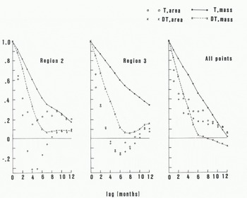
Fig. 4 Autocorrelations of departures from monthly mean ice mass and ice-covered area in regions 2, 3, and the entire domain. Results are shown for the dynamic-thermodynamic simulation DT and the thermodynamic simulation T.

Fig. 5 Time series of departures from 20-year monthly mean ice-covered area in (a) region 1, (b) region 2, (c) region 3, and (d) the entire domain. Results are shown for simulation DT (solid line) and simulation T (dashed line). Horizontal axis indicates year.
Finally, Figure 6 shows the time series of the simulated outflow of ice from the Arctic Basin into the Fram Strait. The plotted values are the mass fluxes across the boundary between regions 3 and 5 (Fig.1). A strong annual cycle is apparent in the mean seasonal outflow, which is much greater in winter and spring than in summer. The seasonality results from both the greater ice thicknesses and the stronger wind-induced ice velocities during the winter/spring portion of the year. A large amount of interannual variability is also apparent in Figure 6. The annual total outflow (km3), for example, ranges from 408 (in 1964) and 541 (in 1963) to 2 109 (in 1962) and 2 118 (in 1975). These large interannual excursions are likely to play significant roles in the mass budgets of the various subregions of the Arctic and the peripheral seas. A more detailed examination of the regional mass budgets is now underway.

Fig. 6 Outflow of ice (km3) from central Arctic into East Greenland Sea. 20-year seasonal means are shown in (a) where Wi is winter, Sp is spring, Su is summer and Au is autumn. Annual totals are shown in (b).
5 Conclusions
This paper has described some initial results from a simulation of northern hemisphere sea-ice fluctuations over a 20-year period. Considerable experimentation remains to be done, especially regarding the sensitivity to the input temperature data and the snow-accumulation rates. Nevertheless, several findings described in section 4 are note-worthy. Perhaps most importantly, the fluctuations of sea-ice mass, both in the entire domain and in individual subregions, are more persistent than are fluctuations of ice-covered area. It follows that anomalies of ice thickness are largely responsible for the evolution of the large-scale anomalies of ice volume or mass. This conclusion is apparent in the results of the complete dynamic-thermodynamic simulation as well as the simulation with only thermodynamics, even though the former produces a much larger seasonal amplitude of the simulated ice mass. However, the inclusion of dynamic processes does tend to introduce more high-frequency variability into the regional (and total) amounts of ice mass.
The time series of the mass and area anomalies contain several multiyear fluctuations within the 20-year simulation period: relatively large amounts of ice in the early and middle 1960s and the middle 1970s, and relatively little ice in the late 1960s and early 1970s. These fluctuations are generally consistent with the high-latitude surface-temperature anomalies of Reference Kelly, Jones, Sear, Cherry and TavakolKelly and others (1982).
The simulated annual ice export from the Arctic Basin into the East Greenland Sea varies by factors of 3 to 4. The role of dynamical processes in the variability of the regional mass budgets has yet to be evaluated in detail, although an adequate description of the large-scale fluctuations is almost certain to involve sea-ice dynamics as well as thermodynamics.
This work is supported by the National Science Foundation, Division of Polar Programs, through grant DPP81-20134. Computing time was provided by NCAR.


