


1. Introduction
Reaction crystallisation, or precipitation (in the context of chemistry), is the formation of crystals via a chemical reaction in a aqueous solution. It is a process employed for producing many products in powder form, such as pharmaceutical powders and pigments. The objective of this process is to produce crystals with specific properties, one of the most important being the particle size distribution (PSD). The driving force for precipitation is supersaturation generated via mixing of reactants. As most precipitation processes take place in turbulent flows, however, the interactions of turbulent mixing with the nonlinear processes of nucleation and crystal growth are complex and not fully understood. In particular, the small-scale action and the molecular diffusion have prominent effects on the species distribution and subsequent build-up of the supersaturated fluid (Bałdyga & Bourne Reference Bałdyga and Bourne1999), which in turn determines the local environment for the crystal formation processes. The ability to understand and control these processes is the key to the capability for tailoring the product PSD to particular applications.
The precipitation of inorganic salts proceeds via ionic reactions that are typically very fast. Nucleation and growth are also fast processes described by strongly nonlinear kinetic expressions. Therefore, one important question is whether a separation of space and time scales between the fluid dynamic and kinetic phenomena is possible. A conventional approach to the modelling of reacting flows is to assume such a separation of scales. Thus, if the kinetic phenomena are much slower than the characteristic flow time scale, a perfectly mixed or lumped model can be employed. At the other end, when kinetic phenomena are much faster than the flow time scale, models based on the assumption that the process is entirely mixing controlled can be employed. These include the mixture fraction-based models commonly employed in turbulent non-premixed combustion (Peters Reference Peters2000; Veynante & Vervisch Reference Veynante and Vervisch2002; Poinsot & Veynante Reference Poinsot and Veynante2005) but also in turbulent precipitation (Bałdyga & Orciuch Reference Bałdyga and Orciuch1997). However, this assumption has not been thoroughly tested in the case of precipitation. Further important questions to be addressed are related to the intermittent nature of nucleation, which can be present in bursts due to the strongly nonlinear nature of its kinetics, and the extent of the spatial zones that control the process outcome. The formation of a large number of small crystals via intense nucleation results in a rapid consumption of reactants as the crystals grow, and, therefore, in a size distribution at the lower end of the spectrum. By contrast, controlled nucleation allows for the supersaturation to be consumed gradually by growth and the formation of larger crystals. The identification of the zones where each process dominates is crucial for the understanding of the evolution of the PSD.
It must be noted that similar research questions appear in several fields where an interaction of transport and kinetic processes is involved. Combustion is one such example, where the modelling of the turbulence-chemistry interaction is of key importance for the prediction of phenomena such as ignition and extinction, and a wealth of modelling approaches have been developed as a result (Peters Reference Peters2000; Veynante & Vervisch Reference Veynante and Vervisch2002; Poinsot & Veynante Reference Poinsot and Veynante2005). Soot formation, in particular, is a problem that involves the interaction of turbulence with chemistry and particle formation and presents many parallels with the problem considered here (Rigopoulos Reference Rigopoulos2019). Another example is flame synthesis of nanoparticles, where the properties of the product depend on the particle size and morphology distribution, which develop as a result of the interaction of fluid dynamics with kinetic processes such as nucleation, aggregation and sintering; a review can be found in Pratsinis (Reference Pratsinis1998), while Raman & Fox (Reference Raman and Fox2016) discuss the modelling issues, particularly with respect to the coupling of chemistry, particle formation and fluid dynamics. Atmospheric aerosols offer another example, as they exhibit a range of particle sizes that determine their health effects; ultrafine particles, for example, can penetrate deep inside the human lungs. The importance of PSDs and their modelling in atmospheric aerosols has been emphasised in treatises such as Hidy & Brock (Reference Hidy and Brock1970), Williams & Loyalka (Reference Williams and Loyalka1991), Friedlander (Reference Friedlander2000) and Seinfeld & Pandis (Reference Seinfeld and Pandis2016). The collision, coalescence and break-up of droplets are instrumental for cloud and rain formation, and atmospheric fluid dynamics plays an important role; for more information, the reader may consult Pruppacher & Klett (Reference Pruppacher and Klett1996) or Khain et al. (Reference Khain, Ovtchinnikov, Pinsky, Pokrovsky and Krugliak2000). Volcanic ash is another form of atmospheric particulates that poses a significant threat for aviation, and where again the interaction of flow and turbulence with a kinetic process (aggregation) is of key importance (Brown, Bonadonna & Durant Reference Brown, Bonadonna and Durant2012; Beckett et al. Reference Beckett, Witham, Leadbetter, Crocker, Webster, Hort, Jones, Devenish and Thomson2020). The balance of nucleation and growth is also important in crystallisation processes other than precipitation, such as the solidification of alloys by cooling (Jarvis & Woods Reference Jarvis and Woods1994).
A model for turbulent precipitation requires coupling of fluid dynamics and precipitation kinetics. Early attempts to employ computational fluid dynamics (CFD) for precipitation were based on lumped methods, where the CFD solution was used for obtaining global mixing parameters such as the turbulent kinetic energy and dissipation rate, which were then used in a phenomenological mixing model for the reacting scalars. In such approaches, the mixer could be divided into compartments assumed to be spatially homogeneous, and mixing at large scales was approximated by the exchanges between compartments. Small-scale mixing, or micromixing, was modelled with phenomenological approaches such as the interaction by exchange with the mean model (IEM) (Villermaux & Devillon Reference Villermaux and Devillon1972; Dopazo & O'Brien Reference Dopazo and O'Brien1974) and the engulfment model – including the subsequent modified engulfment and engulfment-deformation-diffusion (EDD) models of Bałdyga & Bourne (Reference Bałdyga and Bourne1984a,Reference Bałdyga and Bourneb, Reference Bałdyga and Bourne1999). The coupling of compartmental models with CFD can be found, for instance, in the works of Zauner & Jones (Reference Zauner and Jones2000) and Rigopoulos & Jones (Reference Rigopoulos and Jones2001, Reference Rigopoulos and Jones2003a,Reference Rigopoulos and Jonesb) on stirred tanks and bubble column reactors, respectively.
The evolution of the PSD can be described by the population balance equation (PBE). The latter is a partial integro-differential equation for which very few analytical solutions are known, so numerical methods must be employed, and a review of those can be found in Rigopoulos (Reference Rigopoulos2019). The methods that have been employed in coupled CFD-PBE simulations are based on the moment and discretisation approaches. In moment methods, the PBE is transformed into a set of ordinary differential equations for the moments of the distribution, which are then coupled with the equations of fluid dynamics as passive scalars. Only a few low-order moments are computed, typically those associated with physical properties such as particle number density and volume concentration. The advantage of this approach is that the number of additional variables is kept to a minimum. However, the shape of the PSD is not retrieved and the moment equations are unclosed, apart from special cases. Closure approaches include the quadrature method of moments (QMOM) (McGraw Reference McGraw1997) and its further developments, most notably the direct quadrature method of moments (DQMOM) (Marchisio & Fox Reference Marchisio and Fox2005). On the other hand, discretisation (also called sectional) methods retrieve the PSD by applying discretisation techniques such as finite element or finite volume and do not require closure assumptions, but are more demanding in terms of CPU and memory requirements.
Several investigations of turbulent precipitation with coupled CFD-PBE approaches have appeared in the past 20 years. The majority of them have been based on Reynolds-averaged Navier–Stokes (RANS) (Bałdyga & Orciuch Reference Bałdyga and Orciuch2001; Akiti & Armenante Reference Akiti and Armenante2004; Bałdyga, Makowski & Orciuch Reference Bałdyga, Makowski and Orciuch2005; Liu & Fox Reference Liu and Fox2006; Marchisio, Rivautella & Barresi Reference Marchisio, Rivautella and Barresi2006; Woo et al. Reference Woo, Tan, Chow and Braatz2006; Gavi et al. Reference Gavi, Rivautella, Marchisio, Vanni, Barresi and Baldi2007b; Cheng et al. Reference Cheng, Yang, Mao and Zhao2009; Di Veroli & Rigopoulos Reference Di Veroli and Rigopoulos2010; Wu et al. Reference Wu, Fang, Zhao, Wang and Luo2017). Recently, a few studies have also appeared that employ large eddy simulation (LES) (Marchisio Reference Marchisio2009; Makowski & Bałdyga Reference Makowski and Bałdyga2011; Metzger & Kind Reference Metzger and Kind2017; Wojtas, Makowski & Orciuch Reference Wojtas, Makowski and Orciuch2020). The coupling of CFD and PBE accounts for the local driving force (i.e. supersaturation ratio) and spatially varying kinetics that are so important for determining the process outcome, as can be seen in Woo et al. (Reference Woo, Tan, Chow and Braatz2006), Di Veroli & Rigopoulos (Reference Di Veroli and Rigopoulos2010) and Wojtas et al. (Reference Wojtas, Makowski and Orciuch2020) for example.
Despite these investigations, several major issues remain unresolved regarding the coupling of fluid dynamics and precipitation. First, as the smallest scale of mixing is smaller than the grid resolution in RANS and even LES, the micromixing of species is not resolved. The importance of mixing at the molecular level in precipitation has been discussed by Bałdyga & Bourne (Reference Bałdyga and Bourne1999), while the consequence of neglecting micromixing effects has been studied by Marchisio, Barresi & Garbero (Reference Marchisio, Barresi and Garbero2002), where errors of 50 % and 200 % on the mean particle size and total number density, respectively, were reported. The small-scale action has to be taken into account by introducing a micromixing model, like those employed in the lumped methods. Still, good agreement was achieved in some fast precipitation studies without consideration of micromixing (Wei & Garside Reference Wei and Garside1997; Brucato et al. Reference Brucato, Ciofalo, Grisafi and Tocco2000; Cheng et al. Reference Cheng, Yang, Mao and Zhao2009). Therefore, the importance of micromixing was investigated by Marchisio & Barresi (Reference Marchisio and Barresi2003), where it was concluded that its effect depends on the operating conditions and is linked to the Damköhler number. This is in agreement with the findings from Wojtas et al. (Reference Wojtas, Makowski and Orciuch2020) that the sub-grid scales have a negligible effect on the process under fast mixing (kinetics limited) conditions. However, the importance of micromixing effects is still an open question, to which an investigation employing the PBE coupled to a direct numerical simulation (DNS) can provide further insight.
In addition, the effect of turbulence on precipitation is manifested via the effect of concentration fluctuations on the nonlinear nucleation and growth rates. One way of taking them into account is via presumed probability density function (PDF) methods, employed in precipitation by Bałdyga & Orciuch (Reference Bałdyga and Orciuch1997), Bałdyga & Orciuch (Reference Bałdyga and Orciuch2001), Vicum et al. (Reference Vicum, Ottiger, Mazzotti, Makowski and Bałdyga2004) and Makowski & Bałdyga (Reference Makowski and Bałdyga2011). Another approach is the DQMOM-IEM model (Wang & Fox Reference Wang and Fox2004; Marchisio & Fox Reference Marchisio and Fox2005), employed in a RANS (Liu & Fox Reference Liu and Fox2006; Gavi, Marchisio & Barresi Reference Gavi, Marchisio and Barresi2007a; Gavi et al. Reference Gavi, Rivautella, Marchisio, Vanni, Barresi and Baldi2007b) or LES (Marchisio Reference Marchisio2009; Metzger & Kind Reference Metzger and Kind2017) context. Rigopoulos (Reference Rigopoulos2007) proposed a transport PDF approach for accounting for the effect of turbulent fluctuations while retrieving the PSD with a PBE discretisation method. This approach has been applied to turbulent precipitation (Di Veroli & Rigopoulos Reference Di Veroli and Rigopoulos2009, Reference Di Veroli and Rigopoulos2010) as well as to aerosol and soot formation (Di Veroli & Rigopoulos Reference Di Veroli and Rigopoulos2011; Sewerin & Rigopoulos Reference Sewerin and Rigopoulos2017a,Reference Sewerin and Rigopoulosb, Reference Sewerin and Rigopoulos2018, Reference Sewerin and Rigopoulos2019), with the last four studies being in LES context. An interesting finding in Di Veroli & Rigopoulos (Reference Di Veroli and Rigopoulos2009) was that the effect of different unresolved terms relating to the interaction between turbulence and particle formation can be competing, so that a simplified model that neglects all terms yielded an apparently better result than a model where one of these terms was accounted for due to a cross-cancellation of errors. As all those studies were conducted in RANS or LES, however, no definitive conclusion can be made about the effect of fluctuations (or sub-grid fluctuations in the case of LES) and the best way of modelling them. Again, this justifies the attempt to answer these questions via a DNS-based study.
The first DNS-based analysis of turbulent precipitation was carried out by Schwarzer et al. (Reference Schwarzer, Schwertfirm, Manhart, Schmid and Peukert2006) (see also Gradl et al. Reference Gradl, Schwarzer, Schwertfirm, Manhart and Peukert2006; Gradl & Peukert Reference Gradl and Peukert2009), for a series of experiments in a T-mixer conducted by the same group (Schwarzer et al. Reference Schwarzer, Schwertfirm, Manhart, Schmid and Peukert2006). In those studies, the PBE was solved along a number of Lagrangian trajectories at a post-processing level, where the local energy dissipation and the evolution of the concentration of a passive scalar were used for calculating the parameters of a mixing model (a modified version of the EDD model). Apart from the relatively small number of trajectories sampled for statistical convergence (700), the main issue with that approach is the lack of direct coupling between the reactant transport and PBE. The coupling occurs via the consumption of reactants and is instrumental for uncovering the true effect of mixing on crystallisation, which can be crucial in some cases due to the rapid and highly nonlinear kinetics. A methodology for direct coupling of the PBE with DNS was recently presented by Tang, Rigopoulos & Papadakis (Reference Tang, Rigopoulos and Papadakis2020), where a discretised PBE was solved in the whole domain and coupled to the species transport equations via the local consumption due to crystal formation. The approach was validated with the experimental results of Schwarzer et al. (Reference Schwarzer, Schwertfirm, Manhart, Schmid and Peukert2006). This approach paves the way for investigating the effects of turbulent mixing on the PSD by eliminating uncertainties associated with modelling issues.
In the present paper, the methodology of coupling DNS and PBE proposed by Tang et al. (Reference Tang, Rigopoulos and Papadakis2020) is employed to investigate the interaction of turbulence and precipitation. While the objective of that work was to present the methodology and validate it against experimental results from the literature, the present work focuses on analysis of the overlapping of flow, nucleation and growth time scales, the intermittency of these processes and the implications for modelling. The dataset in the present work was obtained by continuing the simulation performed in Tang et al. (Reference Tang, Rigopoulos and Papadakis2020) on the same grid for a longer time, in order to obtain the statistics of the highly intermittent quantities that will be examined here. The Reynolds number is relatively low (1135) but the flow is still turbulent, as the transition  $Re$ value for the geometry simulated here (a T-mixer with a square mixing channel cross-section) is about 400 (Telib, Manhart & Iollo Reference Telib, Manhart and Iollo2004). While DNS studies of such interactions have been carried out in related fields that involve interaction of turbulence and particle formation processes such as soot formation (Bisetti et al. Reference Bisetti, Blanquart, Mueller and Pitsch2012; Wick et al. Reference Wick, Attili, Bisetti and Pitsch2020), aerosol coagulation (Tsagkaridis, Rigopoulos & Papadakis Reference Tsagkaridis, Rigopoulos and Papadakis2022) and cloud microphysics (Grabowski, Thomas & Kumar Reference Grabowski, Thomas and Kumar2022; Macmillan et al. Reference Macmillan, Shaw, Cantrell and Richter2022), such a study has not been performed for reaction crystallisation (to the best of the authors’ knowledge). Furthermore, while there are common threads between reacting flows with particle formation, reaction crystallisation has some important distinct characteristics. The balance and competition between nucleation and growth determines the PSD, the most important process variable, and can only be studied by introducing the effect of the flow field on the PBE. Scale separation is relevant to both processes and underpins many models, some of which (such as the IEM model) are employed in both fields. Other questions to be investigated are the thickness of the nucleation zones and the local rate-determining process, the latter examined via a time scale comparison. Ultimately, the objective of the analysis is to shed light on the role of turbulent mixing in controlling the product PSD.
The paper is structured as follows. The mathematical framework for modelling turbulent precipitation is first presented, followed by a summary of the main features of the numerical approach. After a brief description of the geometry simulated, the results are presented in the following order. First, the flow field, species distribution and PSD are shown. This is followed by an analysis of the intermittent nature of the precipitation process and a definition of suitably filtered time scales, which are subsequently used to analyse the interaction between mixing and precipitation. The thickness of nucleation zones is also examined, and finally an investigation of the local dominant mechanism is conducted, before concluding with a summary of the main findings.
2. Mathematical model of turbulent precipitation
2.1. Governing equations
In the present section the governing equations of reaction crystallisation in a flow field are summarised. The incompressible and constant viscosity form of the continuity and Navier–Stokes equations is
 $$\begin{gather} \frac{\partial u_i}{\partial x_i} = 0, \end{gather}$$
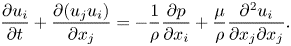 $$\begin{gather}\frac{\partial u_i}{\partial t}+\frac{\partial (u_j u_i)}{\partial x_j} ={-}\frac{1}{\rho}\frac{\partial p}{\partial x_i} + \frac{\mu}{\rho}\frac{\partial^2 u_i}{\partial x_j \partial x_j}. \end{gather}$$
The species transport equations are
 \begin{equation} \frac{\partial C_{\alpha}}{\partial t} + \frac{\partial(u_i C_{\alpha})}{\partial x_i} =\frac{\mu}{Sc_{\alpha}} \frac{\partial^2 C_{\alpha}}{\partial x_i \partial x_i} +R_{\alpha}, \end{equation}
where  $C_{\alpha }$ is the concentration of species
  $\alpha$,
  $R_{\alpha }$ denotes the consumption or generation of this species due to reaction and/or precipitation and
  $Sc_{\alpha }$ is the Schmidt number.
The PBE is a transport equation for the evolution of particle number density, defined as the number of particles per unit volume of particle and unit volume of solution, so that  $n(v;\boldsymbol {x},t)d v$ is the concentration of particles with volume between
  $v$ and
  $v+d v$ at point
  $\boldsymbol {x}$ and time
  $t$. For brevity, the dependence of variables on
  $v$,
$v$,  $\boldsymbol {x}$ and
  $t$ will be omitted in the following. The PBE is
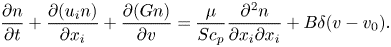 \begin{equation} \frac{\partial n} {\partial t}+ \frac{\partial(u_i n)}{\partial x_i} + \frac{\partial (G n)}{\partial v}= \frac{\mu}{Sc_p} \frac{\partial^2 n}{\partial x_i \partial x_i} + B \delta({v-v_0}). \end{equation}
Here  $B$ is the nucleation rate,
  $v_0$ is the size of the nuclei and
  $G$ is the growth rate. The nucleation and growth rates are functions of the concentrations of chemical species. Therefore, the PBE is coupled with the species transport equations via the concentrations, as well as with the continuity and Navier–Stokes equations via the fluid velocity. The coupling of the PBE with the species transport equations is two-way, as the reaction source term depends on the particle surface area, while it is one-way with the continuity and Navier–Stokes equations for the case of non-inertial particles and constant density flow considered here. Note also that the growth term has the form of an advection term in the particle volume coordinate. The diffusion term represents Brownian motion of particles, and
  $Sc_p$ is the corresponding Schmidt number. It must be noted that, while the PBE for nucleation and growth can be alternatively formulated in terms of particle diameter, here we employ volume as the independent variable because our methodology can also account for aggregation and fragmentation, for which the volume-based formulation is advantageous. In the case considered here, however, aggregation is suppressed due to repulsive electrostatic forces (Eble Reference Eble2000; Schwarzer & Peukert Reference Schwarzer and Peukert2005; Kucher, Babic & Kind Reference Kucher, Babic and Kind2006). This allows the present study to focus on the interplay of mixing with nucleation and growth.
2.2. Precipitation kinetics
The system considered is the precipitation of barium sulphate ( ${\rm BaSO}_4$), formed by mixing barium chloride (
 ${\rm BaCl}_2$) and sulphuric acid (
 ${\rm H}_2{\rm SO}_4$). The chemical equation is
 \begin{equation} {\rm BaCl}_2 + {\rm H}_2{\rm SO}_4 \rightarrow {\rm BaSO}_4 + 2{\rm HCl}. \end{equation}
The driving force for precipitation is supersaturation, a measure of the chemical potential of the reacting ions offset from the thermodynamically stable state. Because of the high ionic strength, the activity-based expression for supersaturation is used (Vicum, Mazzotti & Bałdyga Reference Vicum, Mazzotti and Bałdyga2003), i.e.
 \begin{equation} S=\gamma_{{\pm}} \sqrt{\frac{C_{{\rm Ba}^{2+}_{(free)}} C_{{\rm SO}^{2-}_{4(free)}}}{K_{SP}}}. \end{equation}
The value of the solubility product,  $K_{SP}$, is taken from Monnin (Reference Monnin1999), and the mean activity coefficients
  $\gamma _{\pm }$ are calculated with the modified Debye–Hückel method, more details on which can be found in Appendix A. The reactants are completely dissolved into
  ${\rm Ba}^{2+}$,
  ${\rm Cl}^{-}$,
  ${\rm H}^+$ and
  ${\rm HSO}_4^-$. The
  ${\rm SO}_4^{2-}$ ions are then generated by dissociation of
  ${\rm HSO}_4^-$ and the value of the corresponding equilibrium constant is taken from Schwarzer & Peukert (Reference Schwarzer and Peukert2004). Besides,
  ${\rm BaSO}_4$ tends to form undissociated ion pairs, the actual concentration available for precipitation is therefore less than the compositions in the suspension (Vicum et al. Reference Vicum, Mazzotti and Bałdyga2003). Equation (2.6) therefore only considers the contribution from the free ions. The equilibrium constant for the ion complex formation is taken from Monnin (Reference Monnin1999).
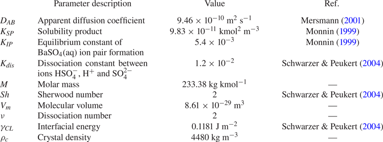
The  ${\rm BaSO}_4$ precipitation kinetics have been studied extensively. Though several kinetic models have been suggested in the literature, each one of them is applicable only over a limited range of conditions. For example, Aoun et al. (Reference Aoun, Plasari, David and Villermaux1996) and Aoun et al. (Reference Aoun, Plasari, David and Villermaux1999) provide a set of values in the expression coefficients for the functional form of the kinetics rate, but the applicable supersaturation range of the established kinetics is still a lot lower than the high supersaturation condition needed for nanoparticle precipitation. The approach in the present study follows the work of Gradl & Peukert (Reference Gradl and Peukert2009), which employs the classical theories of nucleation and growth. We adopt the kinetic expressions in Mersmann (Reference Mersmann2001), which have also been used by several more authors including Gavi et al. (Reference Gavi, Rivautella, Marchisio, Vanni, Barresi and Baldi2007b), Marchisio et al. (Reference Marchisio, Rivautella and Barresi2006), Metzger & Kind (Reference Metzger and Kind2017) under high supersaturation conditions, which is the case here. The values of kinetic parameters are summarised in table 1.
Table 1. Kinetics parameters of  ${\rm BaSO}_4$ precipitation at
  $25\,^\circ$C.
At high supersaturation conditions, primary homogeneous nucleation is the dominant mechanism over secondary and heterogeneous nucleation (Schubert Reference Schubert1998). According to the classical theory, the homogeneous nucleation rate is expressed as (Mersmann Reference Mersmann2001)
 \begin{equation} B_N = 1.5 D_{A B}(\sqrt{K_{S P}} S N_{A})^{{7}/{3}} \sqrt{\frac{\gamma_{C L}}{k T}} V_{m} \exp \left[-\frac{16}{3}\left(\frac{\gamma_{C L}}{k T}\right)^{3} \frac{V_{m}^{2}}{(\nu \ln S)^{2}}\right], \end{equation}
where  $B_N$ is the nucleation rate in terms of particle number, related to the term
  $B$ in (2.4) as
  $B_N = B \, {\rm d} v_0$ (where
  ${\rm d} v_0$ is the interval including the nuclei volume), while
  $N_A$,
  $k$,
$k$,  $D_{AB}$,
  $V_m$,
  $\gamma _{CL}$ and
  $\nu$ are the Avogadro number, Boltzmann constant, apparent diffusion coefficient, volume of
  ${\rm BaSO}_4$ molecule, interfacial energy and dissociation number, respectively. The interfacial energy in the kinetics is taken from Schwarzer & Peukert (Reference Schwarzer and Peukert2004), which is modelled from the adsorption isotherm (Schwarzer & Peukert Reference Schwarzer and Peukert2005). The apparent diffusion coefficient
  $D_{AB}$ in the kinetics expressions describes the migration of the counterion due to the crystal surface charge and is computed from the diffusivity of ions as (Mersmann Reference Mersmann2001)
 \begin{equation} D_{A B}=\frac{(z_{A}+z_{B}) D_{A} D_{B}}{z_{A} D_{A}+z_{B} D_{B}}, \end{equation}
where  $z_A$ and
  $z_B$ is the charge number of ions
  $A$ and
  $B$, respectively. The size of the nuclei depends on the supersaturation. The diameter of the thermodynamically stable nucleus,
  $L_c$, is given by
 \begin{equation} L_{c}=\frac{4 \gamma_{C L} V_{m}}{\nu k T \ln S}. \end{equation}
Crystal growth can be transport controlled or integration controlled, depending on whether it is controlled by diffusion of species towards the particle or by surface processes. The former occurs when the concentration at the particle surface is lower than that in the bulk while the latter occurs when the concentration is the same. For the high supersaturation conditions encountered in this study, growth is transport controlled (Angerhöfer Reference Angerhöfer1994) and can be described by the following expression:
 \begin{equation} G_L = \frac{k_a}{3 k_v} \frac{Sh D_{A B} \sqrt{K_{S P}} M(S-1)}{\rho_{C} L}. \end{equation}
Here  $G_L={\rm d} L/{\rm d} t$ is the linear growth rate and
  $L$ is the particle diameter, while
  $Sh$,
$Sh$,  $M$ and
  $\rho _c$ represent the Sherwood number, molecular weight and density of crystals, respectively. The Sherwood number is the ratio of convection to diffusion mass transfer rate and is taken to be 2, following Schwarzer & Peukert (Reference Schwarzer and Peukert2004). This is an expression for the linear growth rate and involves particle shape factors. The particle morphology reported in the
  ${\rm BaSO}_4$ experiments of the Peukert group (Schwarzer & Peukert Reference Schwarzer and Peukert2002) indicates oval-like and spherical shapes. Therefore, we employ the surface (
 $k_a$) and volume (
 $k_v$) shape factors for spherical particles of
  ${\rm \pi}$ and
  ${\rm \pi} /6$, respectively. In our formulation, we need the volumetric growth rate,
  $G$, which is defined as
  ${\rm d} v/{\rm d} t$, where
  $v=k_vL^3$. By applying the chain rule, we can obtain
  $G$ in terms of
  $G_L$ as
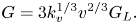 \begin{equation} G = 3k_{v}^{{1}/{3}}v^{{2}/{3}}G_L. \end{equation}
The functional form of the nucleation and growth kinetics exhibits a different dependency on the supersaturation level, as shown in figure 1. The nonlinear behaviour in nucleation and the size-dependent growth rate underpin the complex interactions between these kinetic processes and turbulent mixing that form the subject of the present paper.
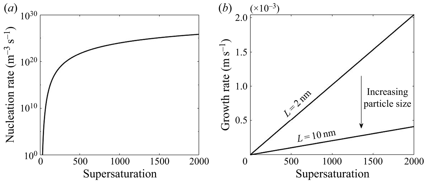
Figure 1. Variation of nucleation and growth rate with supersaturation.
For the purpose of comparing the effects of nucleation and growth and their interactions with flow, we need to define a separate time scale for each of these processes. We adopt the definitions proposed by Bałdyga & Bourne (Reference Bałdyga and Bourne1999), based on the moments of the distribution and the kinetic rates
 $$\begin{gather} \tau_{{N}}=\frac{\displaystyle \int_0^{\infty} n \, {\rm d} v}{B_{N}}, \end{gather}$$
 $$\begin{gather}\tau_{G}=\frac{\displaystyle 3k_{v}^{{2}/{3}} \int_0^{\infty} v n \, {\rm d} v}{\displaystyle k_{a} \int_0^{\infty} G v^{{-1}/{3}} n \, {\rm d} v}, \end{gather}$$
where  $\tau _{N}$ and
  $\tau _G$ are the time scales for nucleation and growth, respectively. The nucleation time scale is defined as the ratio of the total number of particles to the nucleation rate (both are defined as per unit volume of solution) and, thus, indicates the time to form the current number of particles under the current rate, while the growth time scale is defined likewise as the ratio of the total particle volume to the total volumetric growth rate. The latter is obtained by integrating the particle surface area multiplied by the growth rate over particle volume.
3. Numerical method
The results in this study are obtained with the DNS-PBE methodology developed in our previous work (Tang et al. Reference Tang, Rigopoulos and Papadakis2020), hence, only a brief summary will be provided below. The computational implementation is carried out by coupling the in-house DNS code Pantarhei with the in-house population balance modelling code CPMOD. Pantarhei has been used extensively to simulate transitional and turbulent flows in boundary layers, around airfoils, behind fractal grids and inside stirred vessels (Thomareis & Papadakis Reference Thomareis and Papadakis2017, Reference Thomareis and Papadakis2018; Xiao & Papadakis Reference Xiao and Papadakis2017, Reference Xiao and Papadakis2019; Başbuğ, Papadakis & Vassilicos Reference Başbuğ, Papadakis and Vassilicos2018; Paul, Papadakis & Vassilicos Reference Paul, Papadakis and Vassilicos2018; Mikhaylov, Rigopoulos & Papadakis Reference Mikhaylov, Rigopoulos and Papadakis2021). The code CPMOD has been employed for various population balance problems, including aerosol synthesis and soot formation (Sewerin & Rigopoulos Reference Sewerin and Rigopoulos2017a, Reference Sewerin and Rigopoulos2018; Liu & Rigopoulos Reference Liu and Rigopoulos2019; Sun, Rigopoulos & Liu Reference Sun, Rigopoulos and Liu2021).
The flow field is computed by solving the incompressible Navier–Stokes equations (2.1) and (2.2). Because of the small ion mass fraction in the solution mixture, the density and viscosity are assumed to be constant. The equations are discretised with the finite volume method in physical space on a collocated grid. A fractional step method is employed to extract pressures and correct the velocities at the faces of the control volumes, to satisfy continuity. The temporal term in (2.2) is discretised with a third-order backward difference scheme (BDF3). Only orthogonal diffusion terms are treated implicitly, while the non-orthogonal terms are treated explicitly and extrapolated to the next time step with a third-order scheme (EXT3). More details on the BDF3-EXT3 scheme can be found in Tang et al. (Reference Tang, Rigopoulos and Papadakis2020). The convection terms are discretised using a second-order central scheme.
The choice of Schmidt number,  $Sc$, in (2.3) and (2.4) is an important modelling issue, as in reality it can reach very high values (of the order of 1000 for ionic species and even larger for particles), implying that mixing extends to the Batchelor scale,
  $\eta _B$. As
 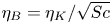 $\eta _B=\eta _K/\sqrt {Sc}$ (Davidson Reference Davidson2004), where
  $\eta _K$ is the Kolmogorov scale, one would need a grid
  $Sc^{3/2}$ times finer than the one needed to resolve
  $\eta _K$ in order to resolve
  $\eta _B$. In our case, this amounts to 664 trillion cells (for
  $Sc=1000$), which is way out of reach of the computational resources available at present or in the forseeable future. Direct numerical simulation studies with high
  $Sc$ have been conducted so far mainly on isotropic turbulence at a relatively low Reynolds number (Donzis & Yeung Reference Donzis and Yeung2010; Donzis et al. Reference Donzis, Aditya, Sreenivasan and Yeung2014; Buaria et al. Reference Buaria, Clay, Sreenivasan and Yeung2021). For more complex flows, the effects of
  $Sc$ on scalar transport were investigated numerically through grid refinement (Derksen Reference Derksen2012) and scale decomposition (Ranjan & Menon Reference Ranjan and Menon2021) although scales of order
  $\eta _B$ were still not fully resolved. These investigations were conducted on passive scalars, however. The use of high
  $Sc$ without resolving the Batchelor scale would lead to numerical oscillations that must be suppressed by a total variation diminishing (TVD) scheme, thus introducing artificial diffusion and having a similar effect to the use of low
  $Sc$. An alternative would be to introduce a micromixing model in a manner similar to LES (van Vliet, Derksen & van den Akker Reference van Vliet, Derksen and van den Akker2005; van Vliet et al. Reference van Vliet, Derksen, van den Akker and Fox2007; Makowski & Bałdyga Reference Makowski and Bałdyga2011). Yet, the applicability of a micromixing model to DNS is debatable as mixing in the inertial-diffusive range has already been accounted for. For these reasons, the use of
  $Sc=1$ is adopted here, although this is an issue that should be further investigated in future work.
The PBE is discretised in the particle size domain with a finite volume method on a composite grid comprising 45 intervals. The composite grid was proposed in Tang et al. (Reference Tang, Rigopoulos and Papadakis2020) in order to accommodate the evolution of the PSD which requires covering a wide range of particle volume, but at the same time provides very good resolution at the nucleation range and good resolution at the particle growth range. The particles are at the nanoparticle range and the Stokes number is very close to zero, so the particle motion can be assumed to follow the fluid motion. The discretised PBE is
 \begin{equation} \frac{\partial n_k} {\partial t}+\frac{\partial(u_i n_k)}{\partial x_i} + \frac{\partial (Gn_k)}{\partial v}= \frac{\mu}{Sc} \frac{\partial^2 n_k}{\partial x_i \partial x_i} + B\delta({v-v_0}), \end{equation}
where  $n_k$ is the discretised number density at section
  $k$ with volume ranging from
  $v_{k-1}$ to
  $v_k$.
The equations for both species and discretised number densities are solved explicitly with a third-order backward difference scheme (BDF3) where the orthogonal diffusion terms are treated implicitly, while the convection and non-orthogonal diffusion terms are treated explicitly, using third-order extrapolation (EXT3). The Gamma differencing scheme from Jasak, Weller & Gosman (Reference Jasak, Weller and Gosman1999) is employed to preserve boundedness of the solution. Furthermore, a TVD scheme is employed for the treatment of the advection-like growth term in the PBE (Koren Reference Koren1993; Qamar et al. Reference Qamar, Elsner, Angelov, Warnecke and Seidel-Morgenstern2006; Qamar, Warnecke & Elsner Reference Qamar, Warnecke and Elsner2009).
The coupling between the reaction and precipitation is performed through the source term  $R_{\alpha }$ in the species transport equations (2.3), which is calculated from the PSD and the nucleation and growth rates as follows:
 \begin{equation} R_{\alpha}=\frac{\nu_{\alpha} \rho_c}{M} \left[B v _0+\sum_{k=1}^m v_{m,k} \left(\frac{\partial G n_k}{\partial v}\right) \, {\rm d} v_k\right]. \end{equation}
Here  $v_{m,k}$ is the midpoint of volume interval
  $k$,
$k$,  $d v_k$ is the size of interval
  $(v_k-v_{k-1})$ and
  $\nu _{\alpha }$ is the stoichiometric factor. Although a transport equation for
  ${\rm BaSO}_4$ is not needed, it is still being solved in order to check mass conservation.
Finally, it must be noted that the advective form in the growth term in the PBE imposes an additional constraint on time advancement, for which a PBE Courant–Friedrichs–Lewy (CFL) number was defined in Gunawan, Fusman & Braatz (Reference Gunawan, Fusman and Braatz2004). The time step required to maintain the PBE CFL number around 0.3 to 0.4 in this study is smaller than the one imposed by the flow CFL number.
4. Geometry and numerical set-up
The turbulent precipitation of  ${\rm BaSO}_4$ nanoparticles in a T-mixer, an experiment documented in Schwarzer et al. (Reference Schwarzer, Schwertfirm, Manhart, Schmid and Peukert2006), is employed as the basis for the present study. This experiment was also simulated by Tang et al. (Reference Tang, Rigopoulos and Papadakis2020), but a longer simulation (13 more flow-through times) was required in order to obtain converged statistics for the intermittent quantities that are discussed in this paper. The T-mixer consists of two inlet pipes with diameter 0.5 mm and a 10 mm (L) long and 1 mm (W) wide square cross-section mixing channel (figure 2). The Reynolds number is 1135 based on the mixing channel width and mean flow velocity, and the flow in T-mixers with a square mixing channel cross-section is turbulent for
  $Re>400$ (Telib et al. Reference Telib, Manhart and Iollo2004). Each reactant is fed from a separate inlet, with concentrations 0.5 kmol m
 $^{-3}$ and 0.33 kmol m
 $^{-3}$ for
  ${\rm BaCl}_2$ and
  ${\rm H}_2{\rm SO}_4$, respectively.
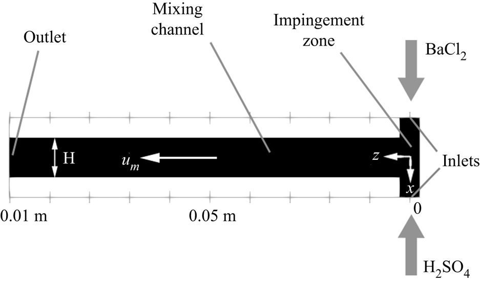
Figure 2. Illustration of the T-mixer geometry.
The simulation employs a uniform Cartesian grid with 21 million cells at 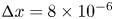 ${\rm \Delta} x=8\times 10^{-6}$ m, which has been found to be sufficient for resolving the Kolmogorov scale in this problem (Tang et al. Reference Tang, Rigopoulos and Papadakis2020); on average, the grid to Kolmogorov scale ratio in the impingement region is less than 1.5 and the maximum is found to be 2.3 at the near wall region. The mixing channel is aligned with the
  $z$-axis, whereas the feed pipes are along the
  $x$-axis, as shown in figure 2. Poiseuille flow is assumed at both inlets, and a convective boundary condition is used at the exit plane. The time step is set to
  $3\times 10^{-7}$ s in order to satisfy the CFL conditions for both flow and population balance, as mentioned in § 3. This time step is two orders of magnitude smaller than the smallest precipitation time scale (which is calculated during the simulation by comparing the nucleation and growth time scales given by (2.12) and (2.13)) and ensures that precipitation is fully resolved.
The simulation was first performed without precipitation in order to obtain a statistically steady flow field (10 flow-through times), at which point reactants were injected. The average and root mean square (RMS) of the flow and precipitation quantities (such as the turbulent kinetic energy, dissipation and supersaturation) were calculated during the simulation and checked at locations featuring strong fluctuations to ensure statistically converged results. The precipitation statistics presented in this work were obtained over 9 flow-through times and their collection started once 4 flow-through times had passed from the moment of reactant injection.
5. Results and discussion
5.1. Flow field
The DNS of the flow field has been validated in our previous work (Tang et al. Reference Tang, Rigopoulos and Papadakis2020) via the simulation of a geometrically similar but 80 times scaled-up T-mixer in which particle image velocimetry (PIV) measurements are available from a hydrodynamic experiment without precipitation (Schwertfirm et al. Reference Schwertfirm, Gradl, Schwarzer, Peukert and Manhart2007). For the T-mixer employed in the precipitation simulations that are analysed here, the spectrum at several locations was calculated in order to confirm that a range of frequencies with a slope of  $-5/3$ is observed, while the terms of the turbulent kinetic energy transport equation were calculated in order to ensure that they balance to an acceptable accuracy. The results of these calculations and the associated discussion can be found in Appendix B. A few hydrodynamic results from the precipitation experiment simulated in this paper are highlighted here, in order to indicate the main features of the flow pattern that are relevant to the following discussion.
The two opposing inlet streams impinge on each other at the entrance of the mixing channel. Figure 3 shows that a global helical vortex is formed at the impingement zone and extends downstream. The helical vortex generates a global mixing environment that sets the stage for the mesoscale and microscale mixing. Small vortices at the channel corner are observed in the mean velocity contours in figure 4. The  $x$-velocity contour indicates small backflows from the opposing jets at the junction with the main channel. These backflows recirculate at the corner of the inlet junctions due to the small vortices, as seen in the
  $y$-velocity contour and, as will be seen in the following discussion, give rise to the supersaturation development in the mixing channel entrances.
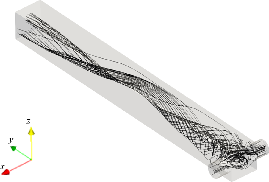
Figure 3. Mean streamlines.
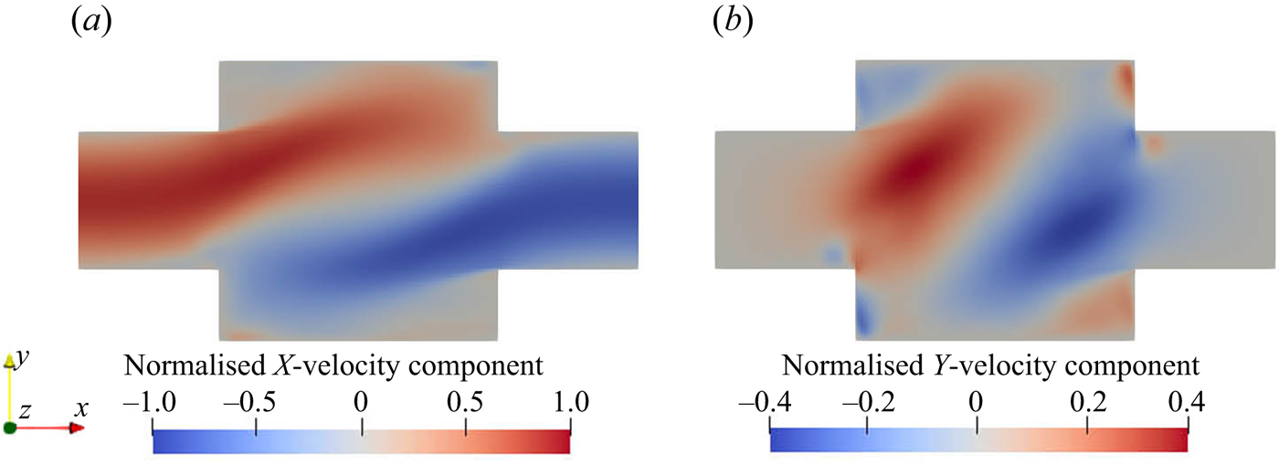
Figure 4. Normalised mean velocity contours of  $x$- (a) and
  $y$-components (b) at the
  $x$–
$x$– $y$ plane at
  $z=0$. The magnitude is normalised by the inlet peak velocity.
Figure 5 shows the contours of the turbulent kinetic energy and its dissipation rate. The rapid increase in turbulent kinetic energy along the inlets shows that the flow experiences a quick transition from laminar to turbulent due to the effect of impinging streams from both sides. Asymmetric contours are observed in both turbulent kinetic energy and dissipation because of the helical flow pattern. The turbulent kinetic energy reaches its peak at the impingement centre and decays downstream in the mixing channel. In addition, the energy dissipation is strong within the entire impingement area and extends to the immediate downstream region. The impingement of the inlet streams and the developed vortical pattern promote the mixing of the reactants in the mixer.
Figure 5. (a) Mean turbulent kinetic energy (m $^2$ s
 $^{-2}$) and (b) dissipation (m
 $^2$ s
 $^{-3}$). Left:
  $x$–
$x$– $y$ plane at
  $z=0$, right:
  $x$–
$x$– $z$ plane at
  $y=0$ (only the first
  $40\,\%$ of the channel is shown).
5.2. Spatial distribution of species and reaction rates
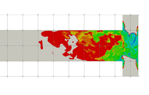
Figure 6 shows the instantaneous and time-average concentration contours of barium and sulphate ions. The barium ions are injected from one inlet, while the sulphate ions are dissociated from the bisulphate injected from the other inlet. Many small structures are observed from the instantaneous contour plot that illustrates the mixing between the reactants. The high concentration streams from the two inlets are moving at opposite directions and circulate around the channel. This suggests that the reactant streams become entrained into the helical vortex as they enter the impingement zone. The concentration of both reactants drops significantly in the downstream of this zone as a result of precipitation within this region.
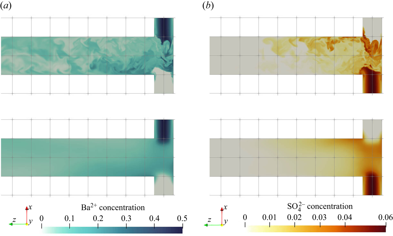
Figure 6. Reactant concentration (kmol m $^{-3}$) contours of
  ${\rm Ba}^{2+}$ (a,c) and
  ${\rm SO}_4^{2-}$ (b,d) (instantaneous (a,b) and mean (c,d)). The
  $x$–
$x$– $z$ plane at
  $y=0$ (only the first
  $40\,\%$ of the channel is shown).
The instantaneous, mean and RMS supersaturation contours at the mid-plane and in the impingement zone are illustrated in figure 7. Due to the fact that the concentrations at the two inlets are not equal, an asymmetric supersaturation distribution builds up along the global helical structure. Beyond the impingement zone, the supersaturation level drops significantly and then decays to zero inside the mixing channel. It is observed from figure 6 that the sulphate ion is completely consumed at the upstream part of the mixing channel (about 30 % of its total length), leading to a sudden drop in supersaturation and thereby a termination of the precipitation process. Thus, beyond this point, the PSD remains unchanged, as can be seen in figure 11 (to be discussed later). Apart from the high supersaturation level in the impingement zone, supersaturation hot spots are observed at the diagonal corners of the inlet junctions (the  $x$–
$x$– $z$ plane in the figures). These spots arise from the recirculations at the bottom corners that bring a high concentration reactant from the opposing jets to the other side, generating a high supersaturation ratio at the inlet wall. In addition, the highest RMS spots are confined within the stream boundaries. These boundaries contain high concentration streams of reactant because of the helical pattern that brings each stream to the other side through the outer part of the impingement zone, and, thus, promotes extreme supersaturation levels within thin regions, as shown in the instantaneous contour plot. However, the stream boundaries are also subjected to strong turbulent fluctuations while the locations of the high supersaturation spots change frequently, leading to the high RMS but a relatively low time-averaged supersaturation field. Notice that the RMS magnitude at the stream boundaries can reach over
  $50\,\%$ of its mean value.
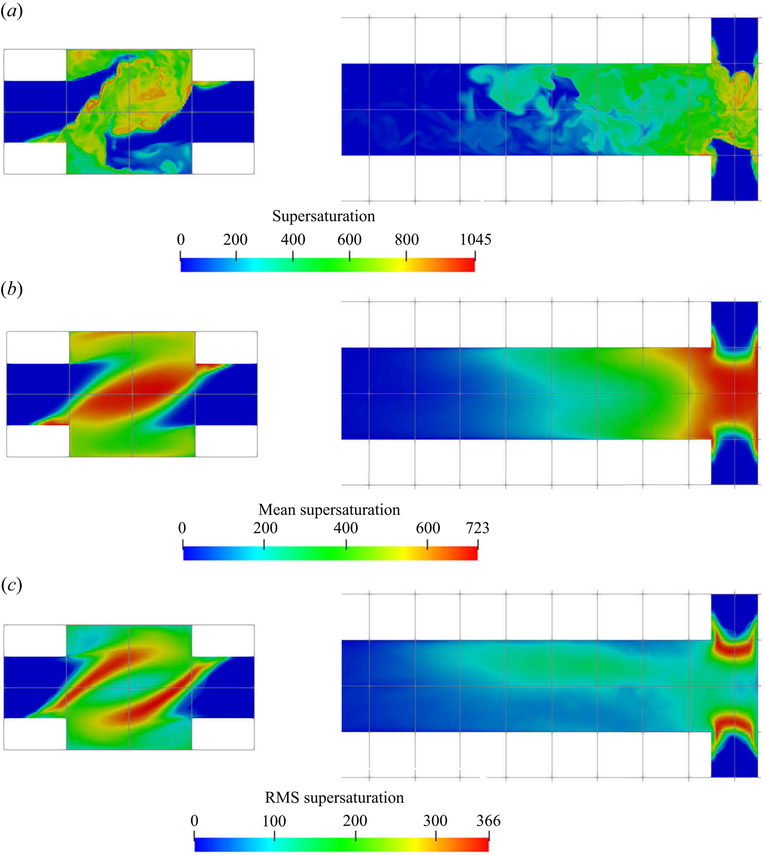
Figure 7. Supersaturation  $[-]$ contours (instantaneous (a), mean (b) and RMS (c)). Left:
  $x$–
$x$– $y$ plane at
  $z=0$, right:
  $x$–
$x$– $z$ plane at
  $y=0$ (only the first
  $40\,\%$ of the channel is shown).
The supersaturation developed in the mixer leads to crystal nucleation and growth, and the reactant consumption rates due to each of these mechanisms are presented in figures 8 and 9, respectively. These are the nucleation and growth contributions to the source term  $R_\alpha$ in (2.3). Both the instantaneous and time-averaged contours show that nucleation has less coverage than growth and usually appears within thin zones, indicating that nuclei formation is confined mainly within the impingement zone. It can also be seen that most of the consumption is due to crystal growth rather than nucleation, as the volume of newly born particles is very small. This implies that the growth acts as a terminating step to the crystallisation process by means of lowering supersaturation. The spatial distribution of the consumption shares similar features with that of supersaturation, such as the fact that the RMS hot spots appear at the stream boundaries. The RMS hot spots for nucleation behave slightly differently than for growth due to the different functional forms of the kinetics of these processes. In particular, the RMS of nucleation consumption at the hot spots located at the stream boundaries are very localised and have magnitude as high as the mean due to the highly nonlinear relation.
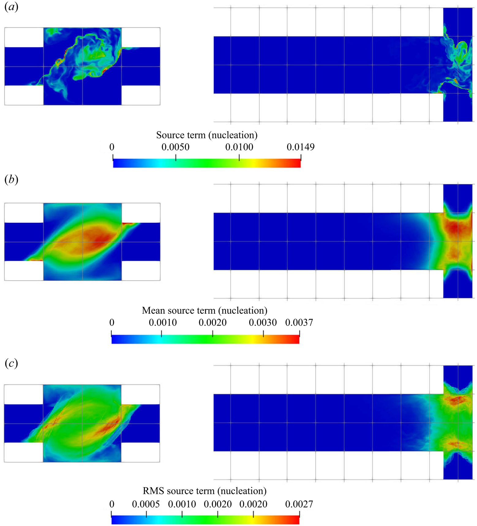
Figure 8. Nucleation consumption term (kmol m $^{-3}$ s
 $^{-1}$); instantaneous (a), mean (b) and RMS (c). Left:
  $x$–
$x$– $y$ plane at
  $z=0$, right:
  $x$–
$x$– $z$ plane at
  $y=0$ (only the first
  $40\,\%$ of the channel is shown).
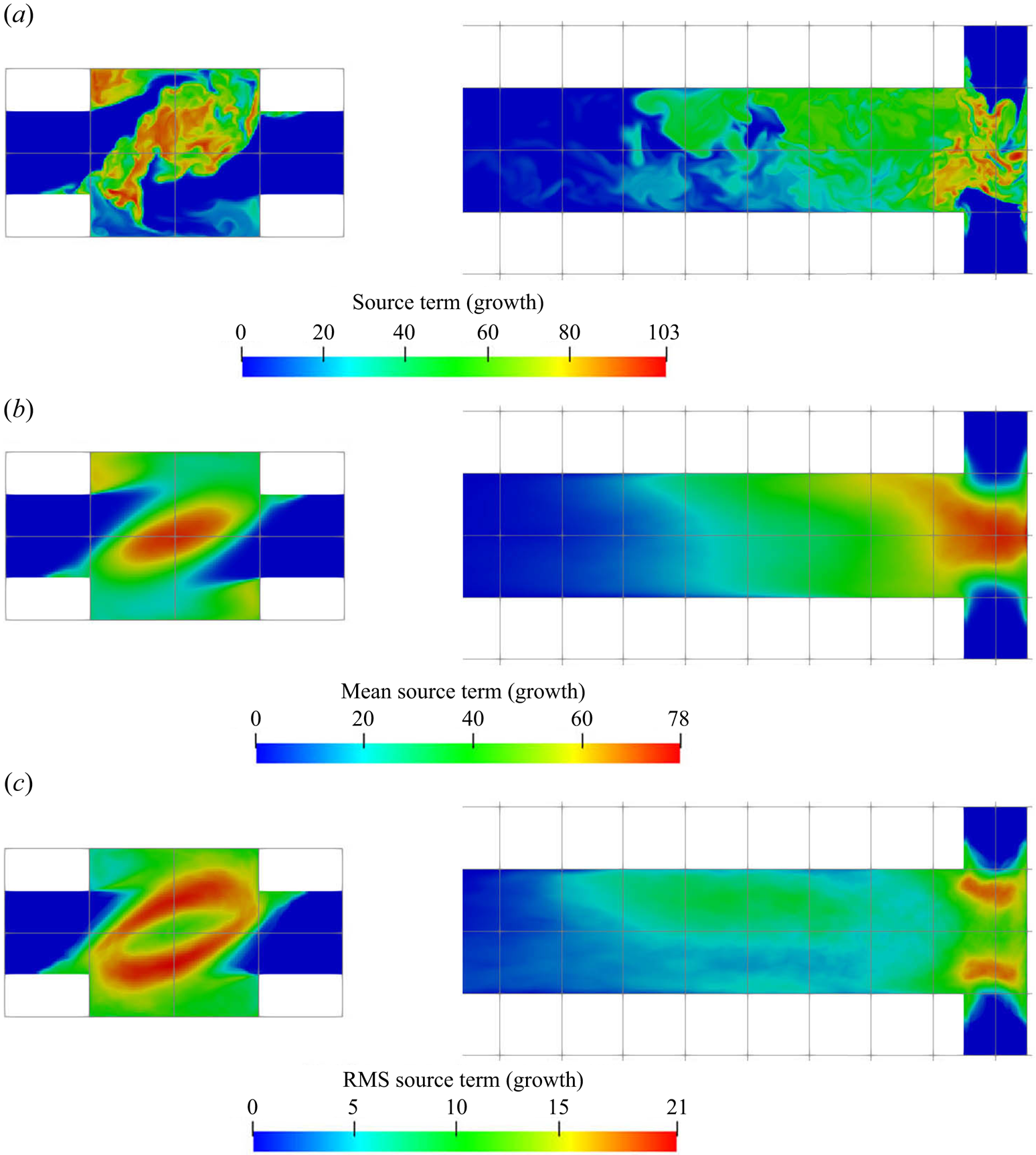
Figure 9. Growth consumption term (kmol m $^{-3}$ s
 $^{-1}$); instantaneous (a), mean (b) and RMS (c). Left:
  $x$–
$x$– $y$ plane at
  $z=0$, right:
  $x$–
$x$– $z$ plane at
  $y=0$ (only the first
  $40\,\%$ of the channel is shown).
Contour plots of the zeroth and first moment of the number density (corresponding to the total number and total volume of particles, respectively) are shown in figure 10. Evidence of the strong precipitation rates at the impingement zone can be seen: a burst of particles is observed in the zeroth moment field as a result of the intense nucleation evidenced in figure 8. The nuclei are then rapidly distributed and their concentration soon evens out. Outside the impingement zone, the number of particles remains approximately constant in the downstream part since the nucleation process has almost terminated there. Meanwhile, the time-averaged first moment reaches half of its final value shortly downstream of the impingement zone and subsequently takes almost four times the mixing distance to achieve the final value. This rapid growth at the early stages can be attributed to high supersaturation and spots with many newly formed particles.
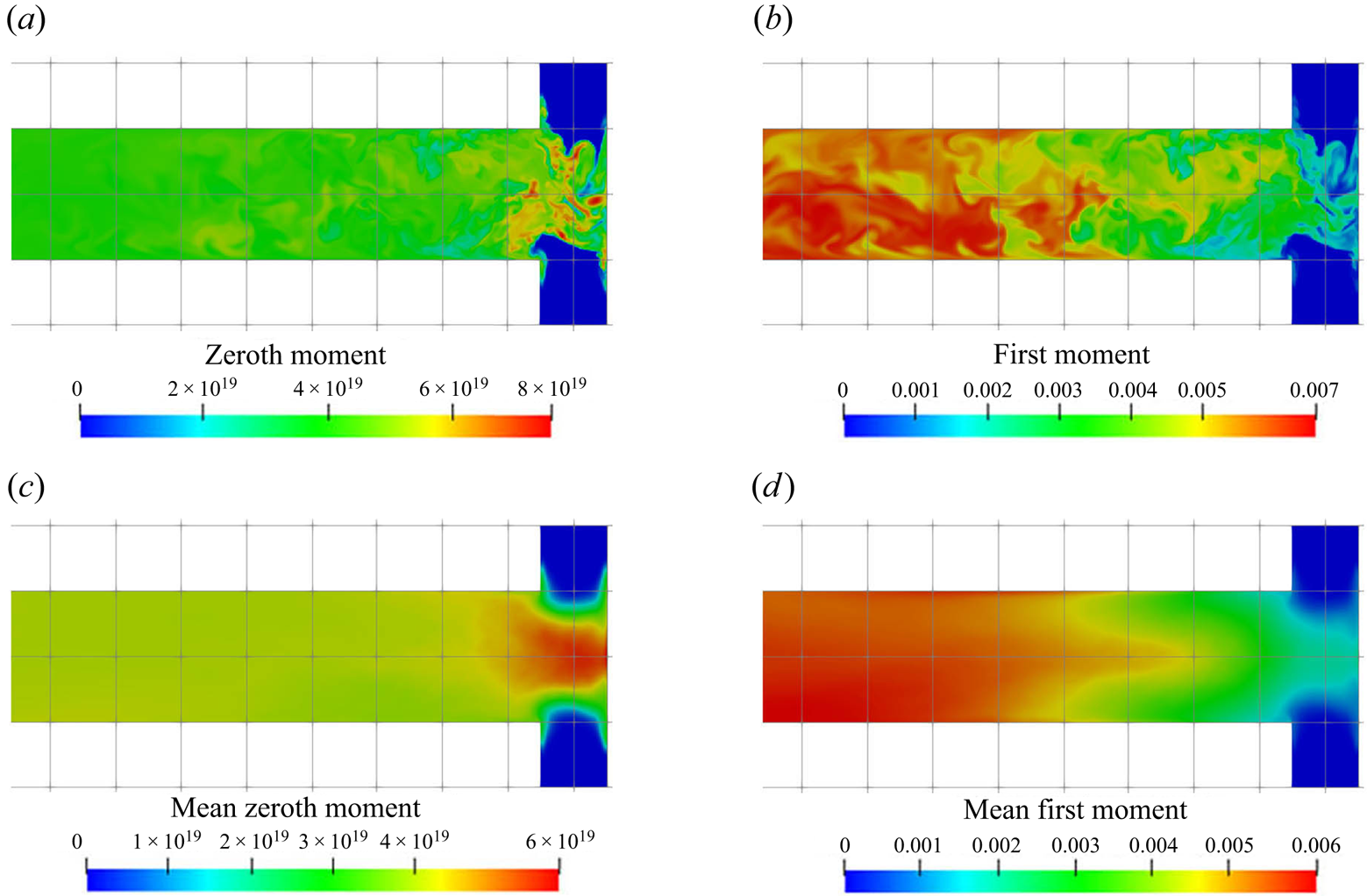
Figure 10. (a,c) Zeroth (m $^{-3}$) and (b,d) first
  $[-]$ moment contours (instantaneous (a,b) and mean (c,d)), representing the total number of particles per unit of solution volume and total crystal volume per unit of solution volume, respectively. Left:
  $x$–
$x$– $y$ plane at
  $z=0$, right:
  $x$–
$x$– $z$ plane at
  $y=0$ (only the first
  $40\,\%$ of the channel is shown).
Although both nucleation and growth are driven by supersaturation, the degree of agreement in their contours with supersaturation behave differently. It is notable (by comparing figures 7a, 8a, 9a and 10) that the contour of the nucleation consumption rate matches closely with that of supersaturation (at the impingement zone, as nucleation is terminated afterwards) while the growth consumption field has better agreement with the first moment over the supersaturation contour. The reason is that the volumetric growth rate depends also on the available crystal surface area. This can be seen by comparing the mean and instantaneous growth contours with that in the zeroth moment contours at the impingement zone (figures 9 and 10): in the mean contours, the growth consumption shares almost identical features with the zeroth moment, except that the amount of growth consumption decays in the downstream while the zeroth moment remains constant since it represents the number of particles formed. Similarly, in the instantaneous contours, growth consumption hot spots appear at locations with high values of the zeroth moment despite the intermediate supersaturation levels, due to the large surface area present there. On the other hand, regions of high supersaturation may feature a high growth rate but still low actual growth if few particles are present. At the impingement, for example, the growth rate is high but the amount of surface area available is very limited. Many new particles are formed, however, in the nucleation bursts induced by the high supersaturation. Afterwards supersaturation drops, while growth starts to take place. This means that the prediction of the spatial distribution of the PSD is essential for correct estimation of the nucleation and growth rates.
Figure 11 shows the evolution of the plane-averaged mean PSD, which is the quantity measured in experiments, from the impingement zone to the outlet. The good matching with measurements (which are available only at the outlet) has been discussed in our previous work (Tang et al. Reference Tang, Rigopoulos and Papadakis2020) and is indicative of the overall validity of the modelling approach, although some uncertainties still remain related to the Schmidt number and kinetics and may explain the remaining discrepancy. In the beginning of the process, the plane-averaged PSD has a slightly asymmetric bell shape with a tail towards the large sizes. Further downstream, the distribution becomes slightly more narrow due to the size-dependent growth kinetics (smaller particles have their size increased at a faster rate), but overall the changes in the plane-averaged PSDs are minor after the impingement zone. This indicates that the PSD is largely determined at the early stages of the process, where supersaturation is high and mixing is critical. This is further discussed in § 5.3.1. Due to the complete consumption of sulphate ions, the consumption maps in figures 8 and 9 suggest that nucleation is terminated immediately after the impingement zone ( $z=0.0005$ m) while the growth of particles is completed further downstream (
 $z=0.003$ m, which agrees with the location where sulphate ion is fully consumed), leaving the mean PSD unchanged along the rest of the mixing channel.
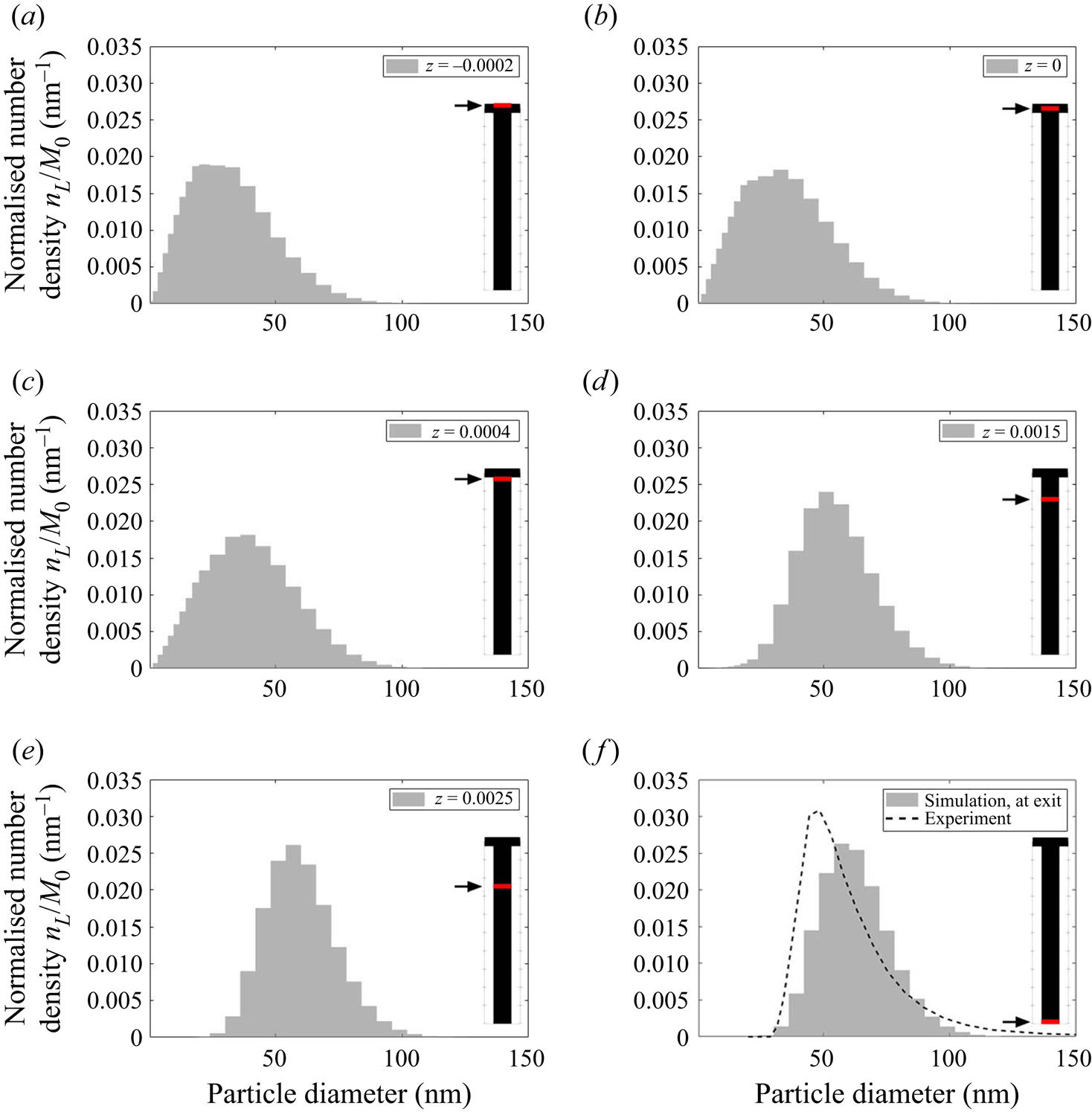
Figure 11. Evolution of the plane-averaged mean PSD, normalised by the zeroth moment, along the mixing channel. The plane location is indicated by the arrows and red lines.
5.3. Analysis of precipitation dynamics
5.3.1. Fluctuations, PDF and intermittent nature of precipitation process
Due to the turbulent nature of the flow in the impinging region, the reactant concentrations and supersaturation are subject to fluctuations, as shown by the time signal of the dissipation rate and supersaturation in figure 12. In the dissipation rate signal, the instantaneous values are several times higher than the time average, indicating highly intermittent behaviour. High intermittency is also observed in both nucleation and growth, due to their nonlinear dependence on supersaturation (figure 1). This behaviour can be seen in the signal of precipitation time scales at the centre of the impingement zone (figure 13). Sharp spikes of large time scales that correspond to slow precipitation rate appear from time to time and nucleation shows more intermittent behaviour than growth under the same supersaturation history, which is attributed to the functional form of its kinetics.
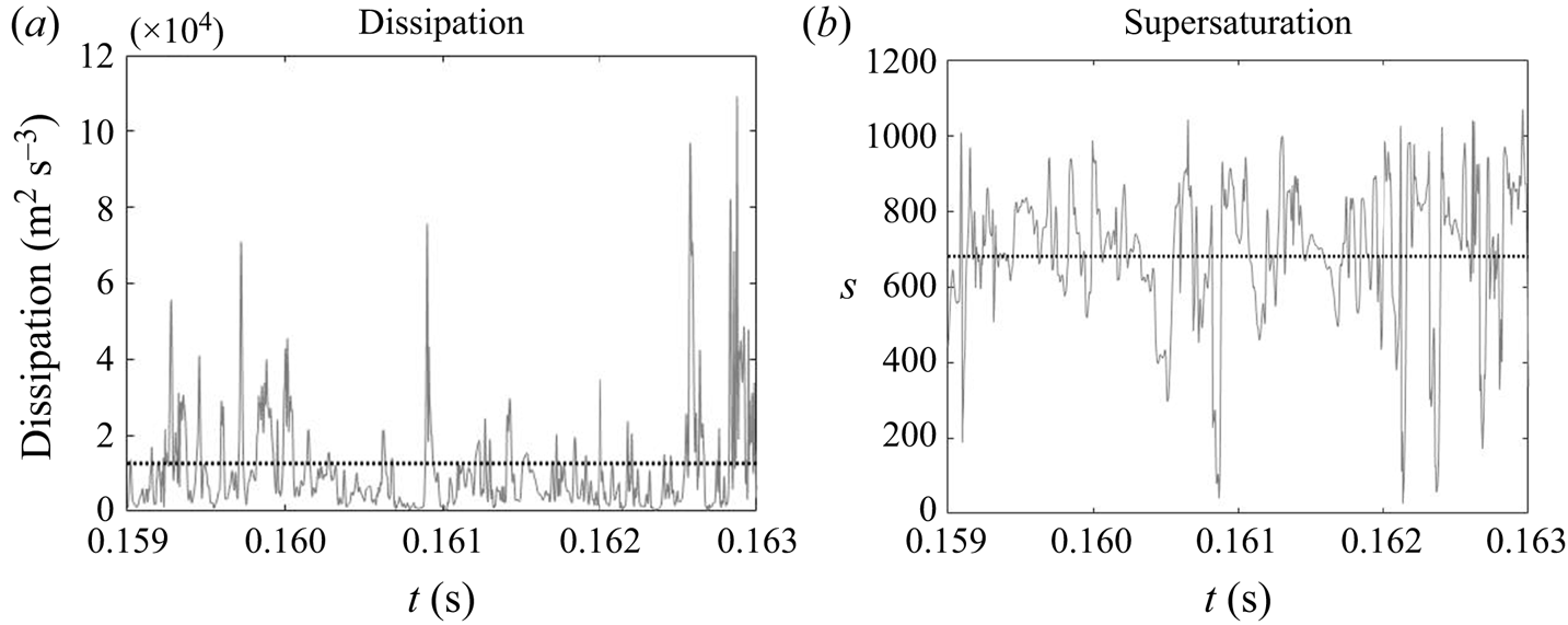
Figure 12. Time signal of energy dissipation and instantaneous supersaturation level at the centre of the impingement region. The time-averaged value is indicated by the dotted line.

The PDF of the time scales signal at the impingement centre is presented in figure 14. For comparison, the PDFs at the channel entrance and at the downstream region are also presented. Generally speaking, both PDFs at the impingement centre and channel entrance show highly asymmetric distribution with the majority of the time scales (both nucleation and growth) being small and much shorter than the mixer flow-through time (indicated by a vertical dashed line). At the impingement centre and at the downstream location, wider distributions are found in the nucleation time scales. This indicates that nucleation contains more slowly reacting events than the growth in which the fluctuation amplifications due to the nonlinear relation with supersaturation makes the nucleation rate variations more obvious. This amplification effect is more apparent in the channel downstream locations where the local time-averaged supersaturation is low. According to figures 8 and 9, the nucleation at this point is weak and almost terminated but the growth still has observable contribution to the PSD despite the slower rate. This leads to a more scattered distribution in both cases with the nucleation one being very wide. Yet, the PDFs at the mixing channel entrance behave differently, where both nucleation and growth contain a wide distribution of time scales that are caused by the high RMS in the fluctuating and moving boundaries illustrated in figures 8 and 9. Comparatively, the growth in this location contains more slow reacting instances that are due to the limiting particle surface area, as will be discussed later in § 5.2.
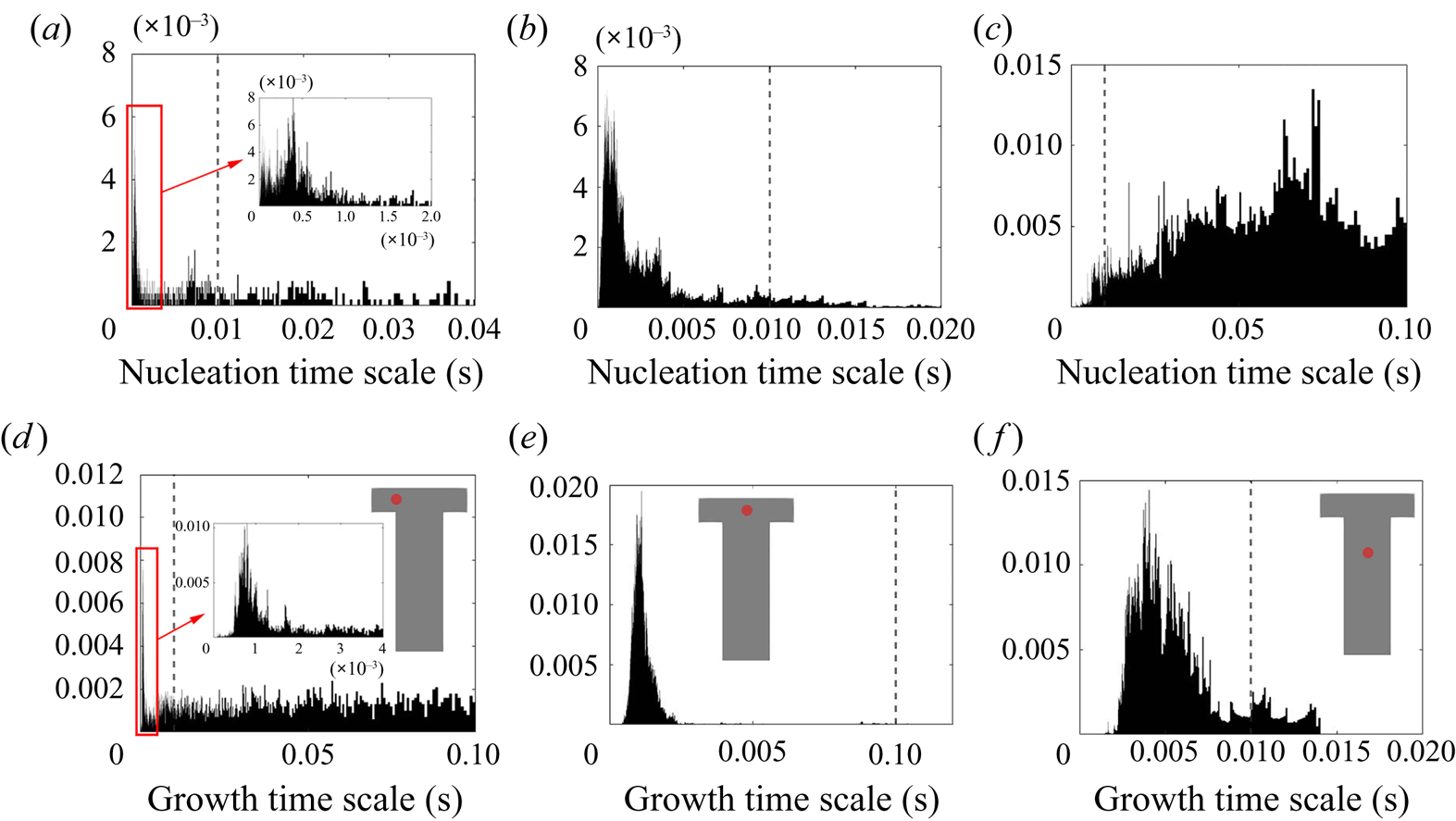
Figure 14. Probability density function of the nucleation (a–c) and growth (d–f) time scales at the mixer channel entrance [ $-$0.0005,0,0] (a,d), impingement centre [0,0,0] (b,e) and mixer downstream [0,0,0.001] (c, f). The probe location is indicated by the red dot and the mixer flow-through time (
 $0.01$ s) is indicated by the vertical dashed line.
Both time scales exhibit a peak in their PDF that represents the most frequent rate on the local PSD evolution. Figure 14 indicates that the peak of the PDF varies spatially. In order to provide further insight, time series data along the  $x$-direction and along the
  $z$-direction for the first
  $10\,\%$ length were collected at 40 and 44 equally spaced probes, respectively. At each point, the most frequently occurring time scale in the PDF (maximum bin value) is selected. The evolution of the PDF peaks for both time scales is presented in figure 15. A symmetric distribution along the
  $x$-direction of the impingement region is observed, as expected. The peak time scales of both nucleation and growth increase along the downstream direction due to the reduction in mean supersaturation. After
  $6\,\%$ of the channel, the peak nucleation time scale is more than one flow-through time, suggesting that nucleation has been terminated; this is consistent with the nucleation consumption contours in figure 8. At the impingement, on the other hand, both peak time scales are of similar magnitude, about
  $10\,\%$ of the flow-through time but generally smaller at the two ends (
 $x/W=\pm 0.5$). Overall, the normalised time scale peak shows much stronger variation for nucleation at the downstream due to amplification resulting from the highly nonlinear dependence of nucleation on supersaturation, leading to a broader PDF and increased intermittency at the downstream region.
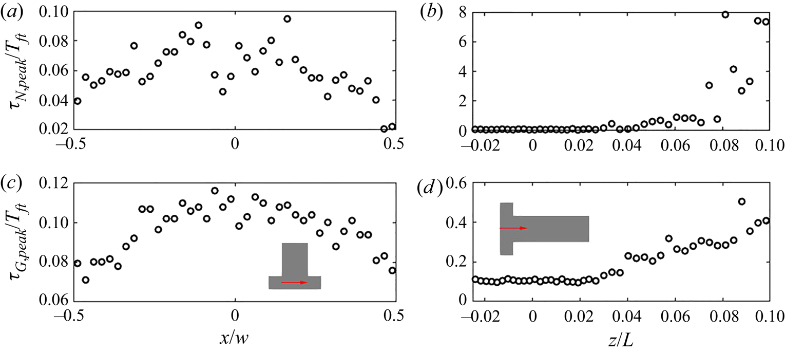
Figure 15. The evolution of peak value in the nucleation (a,b) and growth (c,d) time scales PDF across the channel entrance passing through impingement centre (a,c) measured at probe locations and along the downstream direction (b,d). The precipitation time scales are normalised by the flow-through time ( $T_{ft}=0.01$ s). The
  $z$- and
  $x$- direction distance are normalised by the mixing channel length,
  $L$, and channel width,
  $W$, respectively.
5.3.2. Filtering of precipitation time scales
Time-averaging of the time scales does not provide reliable information due to their high intermittency. As the goal here is to study the interaction between the precipitation kinetics and mixing, the rates at the slowly reacting and non-reacting instances are not important. As such, filtering is performed on the time signal to remove instances of extremely slow rates for the time-average calculation.
The cutoff value for the filtering is chosen to be the flow-through time,  $T_{ft}=0.01$ s, of the mixing channel. This choice can be justified by the following considerations. First, as suggested by figures 8 and 9, the strong reacting regions are concentrated at the impingement, and the PDF information in this region (as shown by figures 14 and 15) has indicated that the majority of the samples are far below the flow-through time. Second, any kinetics time scale longer than one flow-through time of the mixer can be physically considered as a non-reacting instance since the material would have been flushed away from the exit before any reaction effects could be observed. Therefore, a filtered time series can be obtained by filtering out the slow and non-reacting instances from the original series, from which the filtered time averages can be computed. (see figure 16).
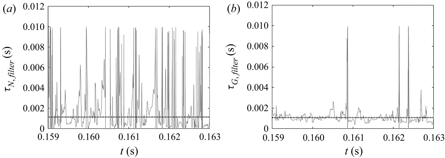
Figure 16. Time series of the filtered nucleation (a) and growth (b) time scales at the impingement centre. The dotted lines indicate the filtered means.
Figure 17 shows snapshots of the instantaneous contours of nucleation and growth time scales. Small time scales indicating strong rates correspond to hot spots and are coloured in red. The overall pattern has a similar structure to the consumption field in figures 8 and 9, and the nucleation field appears to be more localised than that of growth. It can also be seen that a considerable part of the domain is not experiencing reaction at this instance. The nucleation time scale contour in particular is subject to steep changes in the downstream direction and across the inlets.
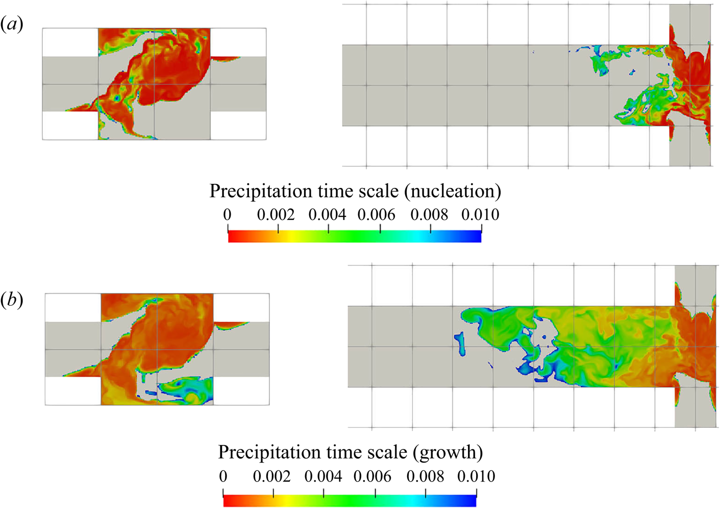
Figure 17. Instantaneous precipitation time scale ( $s$) contours: nucleation (a); growth (b). The red end of the colour bar indicates small values, i.e. fast reaction rates. Values higher than
  $0.01$ s are filtered out and shown in grey. Left:
  $x$–
$x$– $y$ plane at
  $z=0$, right:
  $x$–
$x$– $z$ plane at
  $y=0$ (only the first
  $40\,\%$ of the channel is shown).
Figure 18 shows the filtered time-averaged time scale contours of nucleation and growth at two different planes. As expected, comparison with figure 7 confirms that regions of high supersaturation give smaller time scales that promote a larger influence on the shape of PSD. Direct comparison of the time scale range indicate that both nucleation and growth time scales have a similar order of magnitude in the intense precipitation locations (i.e. impingement). Yet, the time scales on nucleation in the impingement are in general smaller due to more intense hot spots, implying more noticeable nucleation features in the PSD evolution within this area.
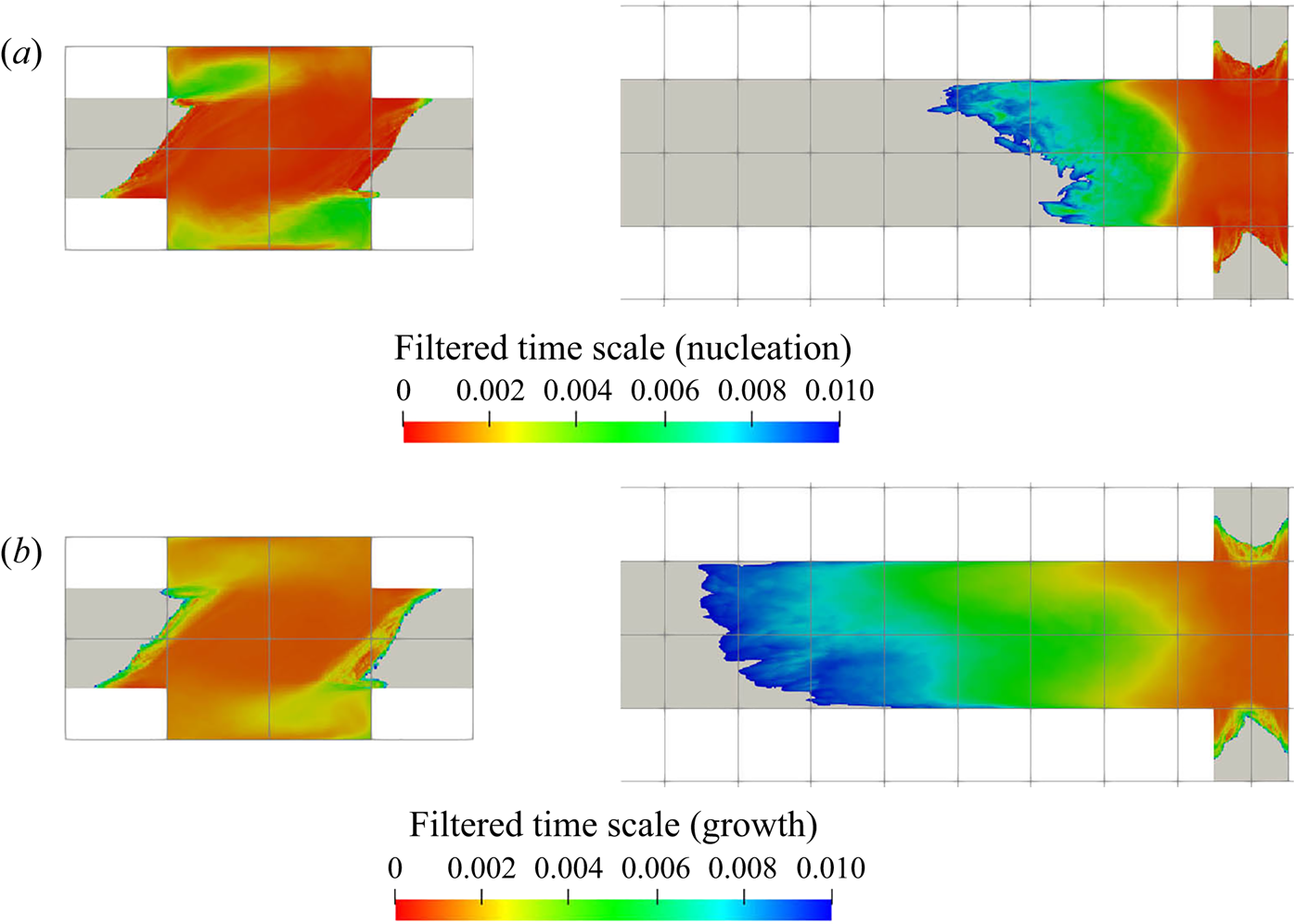
Figure 18. Contours of the time average of filtered time scales ( $s$): nucleation (a); growth (b). The red end of the colour bar indicates small values, i.e. fast reaction rates. Non-reactive regions are shown in grey. Left:
  $x$–
$x$– $y$ plane at
  $z=0$, right:
  $x$–
$x$– $z$ plane at
  $y=0$ (only the first
  $40\,\%$ of the channel is shown).
5.4. Interaction between mixing and precipitation
Having compared the time-averaged filtered time scales of nucleation and growth, we now investigate the interaction between these processes and the flow field. To this end, we define two separate Damköhler numbers ( $Da$), one for each of these processes, as follows:
 $$\begin{gather} D a_{N}=\frac{\tau_f}{\bar{\tau}_{N,filter}}, \end{gather}$$
 $$\begin{gather}D a_{G}=\frac{\tau_f}{\bar{\tau}_{G,filter}}. \end{gather}$$
Here,  $\tau _f$ is the characteristic flow time scale. The process can be thus considered as mixing controlled if
  $Da \ll 1$ and kinetics controlled (by the particular kinetic process) if
  $Da \gg 1$.
It remains to define the flow time scale. One possibility is to employ the engulfment time  $\tau _E$ (Bałdyga Reference Bałdyga2016; see also Bałdyga & Bourne Reference Bałdyga and Bourne1989, Reference Bałdyga and Bourne1999),
 \begin{equation} \tau_{E}=17.3\sqrt{\frac{\nu}{\epsilon}}=17.3\tau_{\eta}.\end{equation}
The engulfment time describes the mixing rate of species  $A$ being engulfed in a zone of rich species
  $B$ due to the most dissipating vortices whose vorticity decays and returns to isotropy in the shortest time (i.e. shortest mean hydrodynamic lifetime) in the energy spectrum. The factor
  $17.3$ comes from the derivation of the engulfment rate in Bałdyga & Bourne (Reference Bałdyga and Bourne1989),
  $E=\ln 2/\tau _w$, where the hydrodynamic lifetime,
 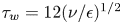 $\tau _w=12(\nu /\epsilon )^{{1}/{2}}$, is taken to be the shortest mean lifetime of an eddy (Bałdyga & Bourne Reference Bałdyga and Bourne1984a). The reciprocal of the engulfment rate is then defined as the engulfment time scale. Note that the engulfment time is one order of magnitude larger than the Kolmogorov time scale (
 $\tau _{\eta }$). This time scale is of relevance to the viscous convective scales, at which precipitation is occurring, and, therefore, can be used to characterise the mixing time scale.
Another set of  $Da$ can be formulated with the eddy turnover time
  $\tau _T$ (
 $k/\epsilon$), on which some commonly employed turbulence models (such as the
  $k$–
$k$– $\epsilon$ model) and mixing models (such as the IEM model) are based. This time scale describes a process at a larger scale (integral scale) than the engulfment time and is thus less relevant to the mixing at small scales. However, as this time scale is often employed in the modelling of micromixing (as, e.g. in the IEM model), it is worthwhile to compare the analysis based on them with the one based on the engulfment time. The differences of the two time scales are illustrated in figure 19. Broadly speaking, the two mixing time scales exhibit a similar order of magnitude in the most turbulent regions, though the engulfment time is smaller everywhere except in the low turbulent kinetic energy regions (cf. figure 5), which are located mainly at the inlet entrances and at some downstream locations where the turbulence has decayed. At the impingement, the engulfment time is around four to six times smaller than the eddy turnover time, which can be expected since the latter describes the decay of larger-scale vortices. In the following, the sets of
  $Da$ based on both time scales will be juxtaposed.
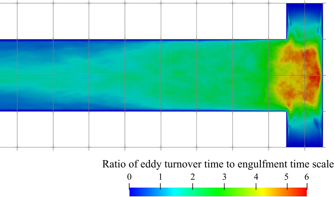
Figure 19. Ratio of eddy turnover and engulfment time;  $x$–
$x$– $z$ plane at
  $y=0$ (only the first
  $40\,\%$ of the channel is shown).
Figures 20 and 21 present the  $Da$ contours based on the engulfment time
  $\tau _E$ and eddy turnover time
  $\tau _T$, respectively. The nucleation and growth time scales are both comparable with each of the two flow time scales at the regions of intense precipitation. This indicates that the process is neither mixing nor kinetics controlled. A high concentration of reactants entrained into vortices can lead to nucleation bursts, but they can also get dispersed in a short time by the mixing. Without mixing, the nucleation bursts would remain for a long time because the reactant consumption due to nucleation is very low (see § 5.2). Capturing such events is necessary for an accurate prediction of the PSD.
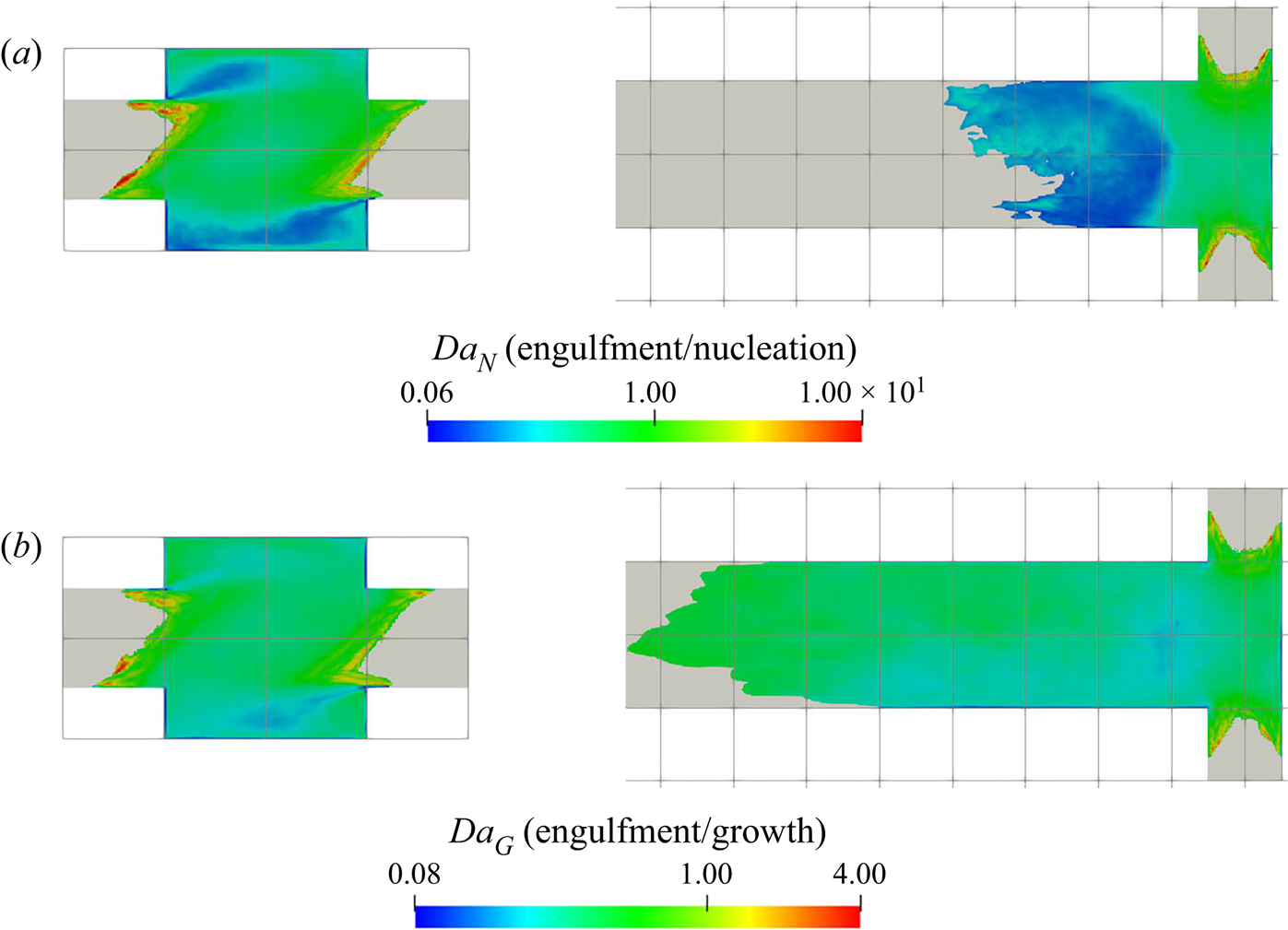
Figure 20. Damköhler number map based on the engulfment time: nucleation (a); growth (b). Non-reactive regions are shown in grey. Left:  $x$–
$x$– $y$ plane at
  $z=0$, right:
  $x$–
$x$– $z$ plane at
  $y=0$ (only the first
  $40\,\%$ of the channel is shown).
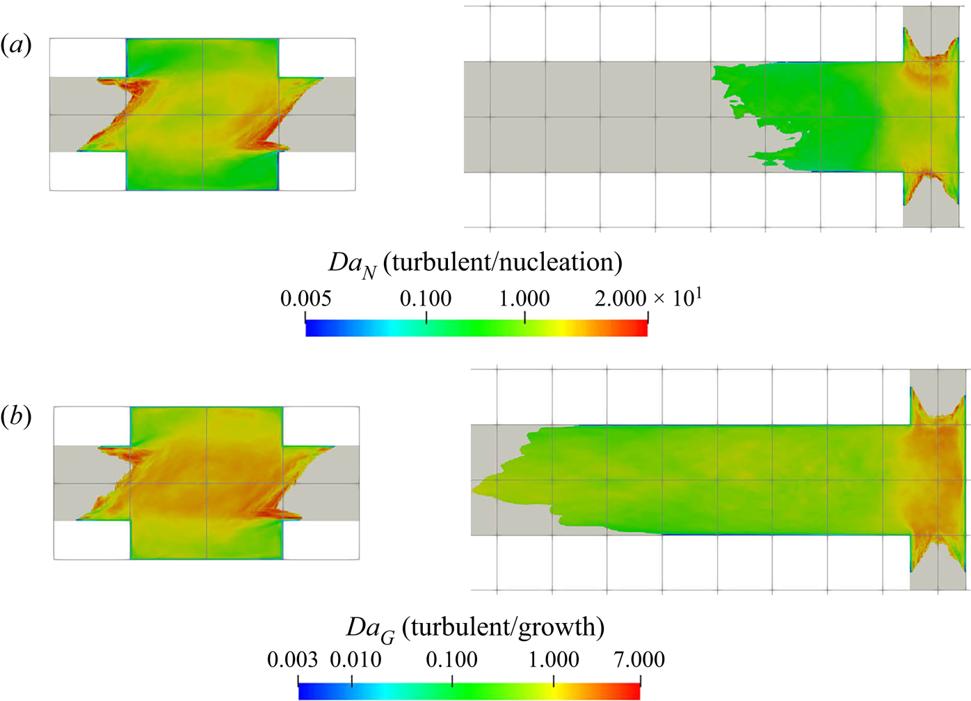
Figure 21. Damköhler number map based on the eddy turnover time: nucleation (a); growth (b). Non-reactive regions are shown in grey. Left:  $x$–
$x$– $y$ plane at
  $z=0$, right:
  $x$–
$x$– $z$ plane at
  $y=0$ (only the first
  $40\,\%$ of the channel is shown).
For both definitions of  $Da$, the values are around unity for a significant part of the domain, with the
  $Da$ based on
  $\tau _E$ being biased on the mixing-controlled side and the one based on
  $\tau _T$ on the kinetics-controlled side. While the difference between the two is small in this case due to the relatively low Reynolds number, considering that the
  $\tau _{E}$ is of the order of the Kolmogorov scale and
  $\tau _{T}$ is of the order of the integral scale (Pope Reference Pope2000), the difference between their resultant
  $Da$ is likely to increase for high
  $Re$ cases as the ratio between the
  $\tau _{E}$ and
  $\tau _{T}$ becomes larger. This has important implications for precipitation models, as the eddy turnover time is used in RANS models and in micromixing models such as the IEM (which is also used in LES). The engulfment time reflects better the influence of the small scales, which are crucial for the reactive processes in crystallisation, especially nucleation.
5.5. Nucleation zone thickness
Due to its nonlinear relation with supersaturation and strong intermittency, the nucleation is very localised. This results in many thin reaction zones with strong nucleation bursts. These zones must be properly resolved for an accurate prediction of the PSD. Furthermore, it is worth investigating the thickness of these zones and comparing it with the Kolmogorov length scale. In the context of combustion, the thickness of such reaction zones is very important for determining the combustion regime and applicability of models that involve decoupling of chemistry and flow (Peters Reference Peters2000; Veynante & Vervisch Reference Veynante and Vervisch2002; Poinsot & Veynante Reference Poinsot and Veynante2005). Such an investigation, however, has not been carried out for reaction crystallisation so far.
The nucleation zone thickness ( $l_n$) is obtained from spatial data at 30 uncorrelated time instances. The location of the line probe where the sample data are collected is illustrated in figure 22, where the nucleation zones are also shown. In order to quantify the nucleation zone thickness, we consider the derivative of the nucleation rate. A peak and a trough in the first-order derivative appear at the left and right side of each peak, respectively, and the distance between them is taken to be the nucleation width. Many thin nucleation bursts can be observed. From the 30 instances, 239 peaks were identified, giving a mean, standard deviation, maximum and minimum thickness of
  $2.9 \times 10^{-5}$ m,
  $1.2 \times 10^{-5}$ m,
  $9.6 \times 10^{-5}$ m and
  $1.6 \times 10^{-5}$ m, respectively. The PDF of the collected samples is plotted in figure 23, which shows an asymmetric distribution. The minimum thickness is higher than the grid resolution and the mean thickness is resolved with five cells, so the grid resolution is sufficient to ensure that the nucleation bursts are properly captured. It must also be borne in mind that the assumption of
  $Sc=1$ has been made in the present simulation, which is likely to have an effect on the thin nucleation layers.
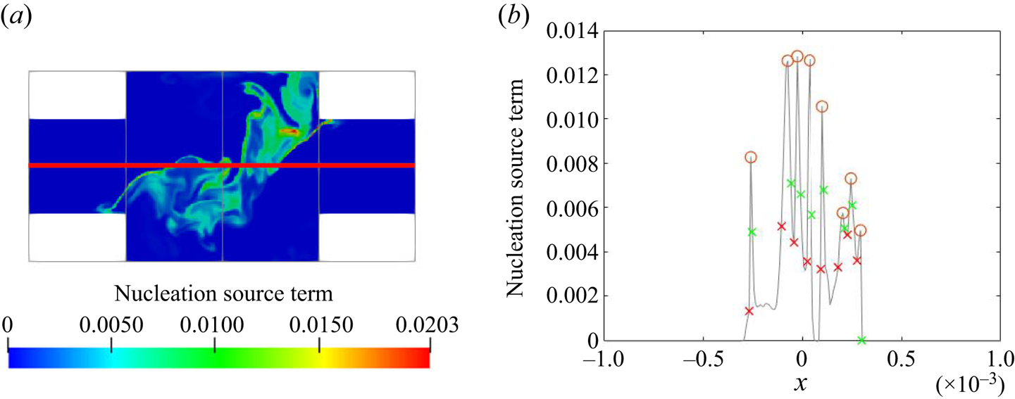
Figure 22. Contour plots of the instantaneous nucleation source term (kmol m $^{-3}$ s
 $^{-1}$). The probe points are located on the horizontal red line at the
  $x$–
$x$– $y$ plane at
  $z=0$ (a). Peaks of nucleation source term are identified by the circle markers (b). The peak and troughs in the first derivative around each source peak are indicated by the red and green cross markers, respectively. The peak width is defined by the distance between the cross markers.
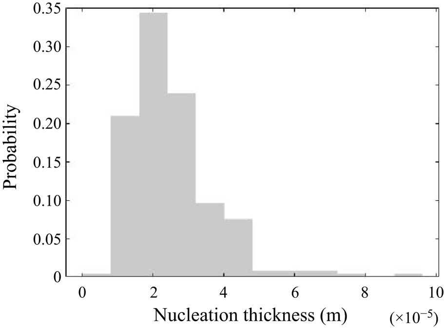
Figure 23. Probability density function of nucleation zone thickness.
A dimensionless ratio can be defined by dividing the nucleation thickness by the local Kolmogorov length scale ( $l_n/\eta _{k}$). This gives a mean, standard deviation, maximum and minimum ratio of 6.1, 2.9, 19.1 and 1.2, respectively. The fact that a range of this ratio is considerably greater than unity indicates that the transport by turbulence penetrates into the intense nucleation zones. Since the reactant consumption rate due to nucleation is very small even at high nucleation rate (see § 5.2), the reactant concentration is not likely to drop solely due to nucleation and the high concentration can only be broken down by turbulent transport. As such, the penetration of turbulence into precipitation decomposes nucleation bursts via dilution. This could have strong effects on the final PSD and should not be overlooked. Furthermore, the difference between the maximum and minimum ratio spans over one order of magnitude, which indicates the presence of a range of spatial scales in nucleation. Therefore, the assumption of scale separation and consequent decoupling of chemistry and flow in precipitation cannot be justified for nucleation and models based on it may overlook important small-scale interactions.
5.6. Local dominant mechanism
In this section we employ the ratio of precipitation time scales to construct a map of regions where precipitation is dominated by nucleation or growth, or where the two processes are balanced. The contour of the instantaneous ratio  $\tau _N/\tau _G$ is shown in figure 24(a). Based on this map, the domain can be divided into three zones with respect to the time scale ratio, where the mechanism with the smallest time scale dominates the PSD evolution. The process changes from nucleation dominated in the impingement to growth dominated in the downstream region. The ratio in the mixing channel is particularly high since nucleation stops there, allowing growth to fully dominate the process. Additionally, during the transition from the nucleation-dominated region to the growth-dominated region, the time scales of both mechanisms are comparable, implying similar effects on the PSD.
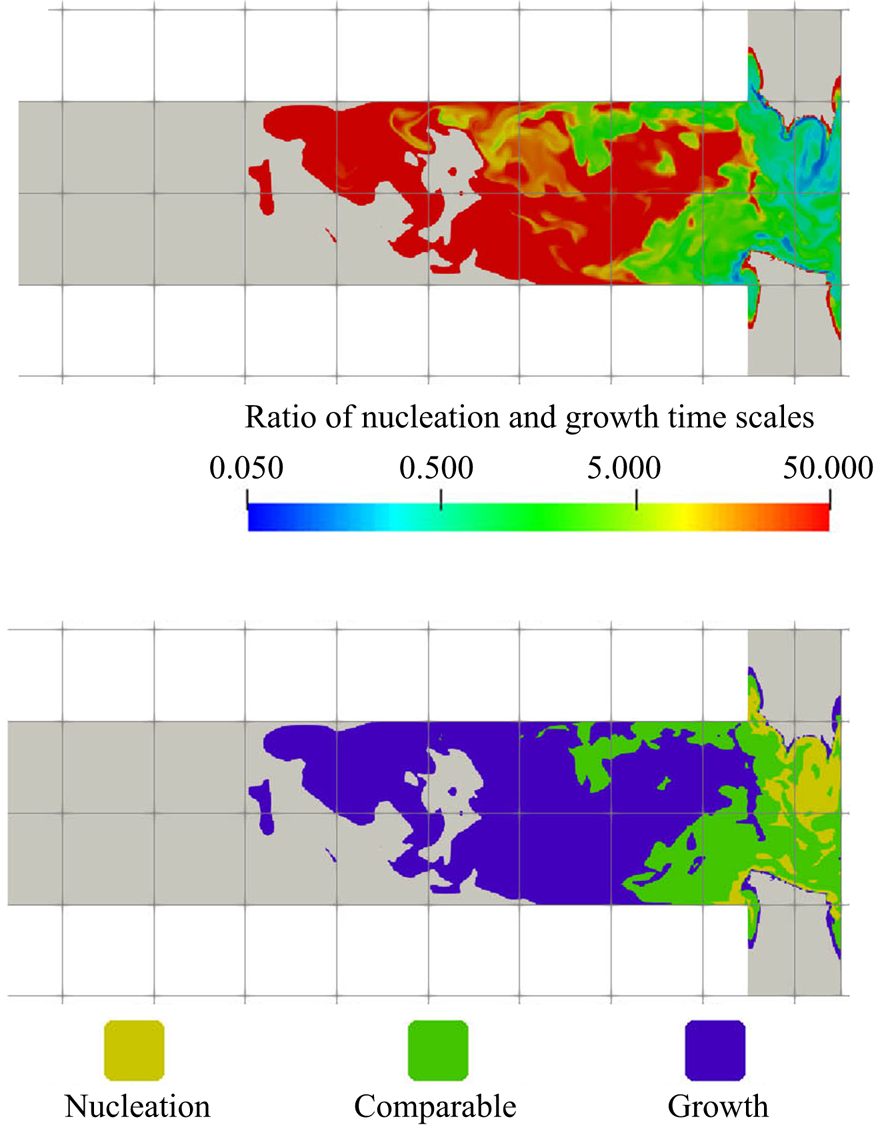
Figure 24. (a) Ratio of  $\tau _N$ to
  $\tau _G$. The maximum value is set to 50 for the purpose of illustration. Non-reactive regions are shown in grey; (b) dominant zones classified by colour (blue: growth; yellow: nucleation; green: comparable time scale), with non-reactive regions shown in grey
  $X$–
$X$– $z$ plane at
  $y=0$ (only the first
  $40\,\%$ of the channel is shown).
It should be noted that the local dominant mechanism is identified mainly based on instantaneous snapshots rather than time-averaged fields to emphasise the importance of the highly intermittent nucleation behaviour, which is likely to be averaged out in a time-averaged field. To illustrate this, the local PDF of the filtered time scale ratios at the three locations indicated in figure 14 is presented in figure 25. The  $x$-axis is in logarithmic scale to show the extreme nucleation instances. It can be seen that the PDFs could span over a fewer orders of magnitude and the shapes are highly skewed regardless of the location. Averaging is therefore likely to be dominated by the large ratio (week nucleation) side given the high standard deviation in the PDF. The time-averaged time scale ratio and the standard deviation at the probe locations in the
  $x$- and
  $z$-directions are presented in figure 26, where the competition between nucleation and growth appears to be less intense, although the transition of the dominant mechanism can still be observed along the downstream direction. Yet, at all probe locations, the time-averaged ratio is merely within one order of magnitude, whereas the instantaneous ratio in figure 24 shows much larger differences.
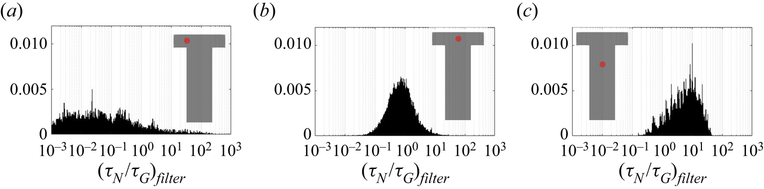
Figure 25. Probability density function of the time scale ratio between nucleation and growth at the mixer channel entrance [ $-$0.0005,0,0] (a), impingement centre [0,0,0] (b) and mixer downstream [0,0,0.001] (c). The probe location is indicated by the red dot and the
  $x$-axis is represented in logarithmic scale.
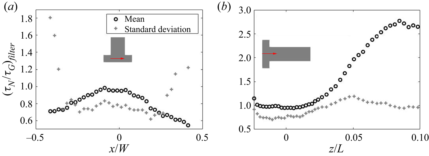
Figure 26. The evolution of the mean ( $o$) and standard deviation (
 $+$) of the nucleation to growth time scale ratio across the channel entrance passing through impingement centre (a) measured at probe locations and along the downstream direction (b). The
  $z$- and
  $x$- direction distance are normalised by the mixing channel length,
  $L$, and channel width,
  $W$, respectively.
Although, as shown in § 5.2, the pattern in growth consumption contour does not always follow supersaturation, the final map still shows good matching. This is because nucleation occurs only at high supersaturation, which leads to a smaller nucleation dominant region. In a similar way, any regions that do not have nucleation are growth dominated. This effect is evident in figures 11 and 10, where it can be seen that the PSD moves towards larger scales without increases in the zeroth moment. At this stage, the ions tend to be consumed by particle growth.
Being able to identify the dominant mechanism in each zone helps in understanding the underlying effects that guide the PSD evolution. In § 5.2 it was shown that most of the reactants are consumed via growth. Since growth only takes place on the particle surfaces, controlling the number of nuclei formed at the early stages has major effects on the PSD. Increasing the extent of the nucleation-dominated regions helps to suppress the growth of large particles, which in turn reduces the final particle sizes as more particle surface is available for growth at a small particle size interval. The key on tailoring the PSD is therefore the control of the extent of the nucleation-dominated regions.
The dominant mechanism map helps to illuminate the role of mixing in reaction crystallisation. The spatial distribution and extent of the dominant zones is determined by mixing. In a laminar flow, a nucleation-dominated zone will be limited to the diffusion zone, resulting in fewer and larger particles. Turbulence introduces vortices of different sizes that help to redistribute high supersaturation zones and to spread out the nucleation-dominated regions, thus resulting in more nucleation and smaller particles. A fully mixed system, however, may feature less nucleation due to the dilution of supersaturation.
6. Conclusions
The objective of this paper was to elucidate the role of turbulent mixing and the interactions of turbulence with the kinetic processes of nucleation and growth in reaction crystallisation. The analysis employed a coupled DNS and discretised population balance approach developed by Tang et al. (Reference Tang, Rigopoulos and Papadakis2020) and was conducted on the  ${\rm BaSO}_4$ nanoparticle precipitation in a T-mixer investigated experimentally by Schwarzer et al. (Reference Schwarzer, Schwertfirm, Manhart, Schmid and Peukert2006). Such analyses have been carried out in several fields that involve interaction of turbulence and particle formation processes such as soot formation, aerosol coagulation and cloud microphysics, but this has not been the case with reaction crystallisation (to the best of the authors’ knowledge), which has several distinct characteristics. The most important is the presence of two reactive processes, nucleation and growth, their competition determines the PSD, which is the most important property of the product. This competition, and the effect of mixing which sets the stage for it, can only be investigated by coupling the population balance with fluid dynamics and examining how flow field features affect the nonlinear processes in the PBE. The interaction of flow and nucleation, in particular, has parallels in atmospheric aerosol and cloud formation.
Precipitation was found to take place mainly within the impingement zone, where strong turbulence is present and a large-scale helical vortex is formed. Due to the amplification of the nonlinear kinetics, the fluctuations in reactant concentrations lead to a highly intermittent precipitation rate. The PDFs of nucleation and growth time scales show higher intermittency in nucleation than in growth, making the former a more localised process. Due to the highly intermittent time scales, filtering was performed to remove the slow and non-reacting instances, and the investigation of the mixing-precipitation interaction was performed through suitably defined Damköhler numbers based on time-average filtered time scales, separate for nucleation and growth. For both mechanisms, comparable turbulence and kinetic time scales were observed throughout the domain, indicating that the process is neither mixing nor kinetics controlled. The breakdown and formation of reaction hot spots by mixing and the consumption of reactants, therefore, needs to be properly resolved. The use of two flow time scales, the engulfment and the eddy turnover time, in the definition of a Damköhler number was investigated. The difference between these two time scales is expected to increase with the Reynolds number and this has implications for precipitation models that employ the eddy turnover time, as the engulfment time is more characteristic of the small-scale motion where precipitation occurs and, thus, more relevant for investigating the rate-determining mechanism.
Nucleation plays a vital role in reaction crystallisation, as it determines the number of seeds generated. A large number of seeds leads to a distribution leaning towards the smaller sizes, as the supersaturation is rapidly consumed. In regions of intense supersaturation, nucleation bursts were observed that were confined to extremely thin zones. Resolving these zones is therefore indispensable for a correct prediction of the PSD. A comparison of the nucleation burst thickness in the impingement zone to the Kolmogorov scale indicated that turbulence transport penetrates into the intense precipitation zone. This suggests that turbulence may have an important influence on nuclei formation, and that the use of models that assume scale separation between precipitation and turbulence may not capture these physics.
On the other hand, growth is the mechanism that eventually terminates the precipitation process, as it accounts for the majority of the consumption and, therefore, the weakening of nucleation, which has a strong dependence on supersaturation. The pattern in the growth consumption contour did not fully match that of supersaturation, due to the additional dependency of growth on the particle surface area. The correct prediction of the local PSD is therefore important for obtaining the correct growth rate.
The difference in the dependence of nucleation and growth with supersaturation leads to different local dominant mechanisms. The zone where each process is dominant was identified via the precipitation time scale ratio. Good matching was found between the dominant mechanism map and the supersaturation contour. The matching helped in identifying the range of supersaturation where each mechanism dominates.
The results of this study provide evidence towards answering the fundamental question of how mixing controls the PSD in reaction crystallisation. The development of the PSD is a result of the competing mechanisms of nucleation and growth, the former becoming dominant only at high supersaturation and the latter terminating the precipitation process, and the interaction of these mechanisms with turbulent mixing can be analysed with the aid of appropriate Damköhler numbers. From this perspective, the PSD is related to the extent of the nucleation zones. The faster the mixing, the larger the contact area between reactant species where supersaturation develops. This eventually increases the extent of the nucleation dominant zone and provides more particles to consume the remaining reactants via growth, leading to smaller particles in the distribution. Therefore, broadly speaking, mixing feeds the supersaturation build-up and subsequently controls the distribution of rate-determining mechanisms.
There are still unanswered questions, such as the effect of the Batchelor scales and the interactions of flow and kinetics under different Damköhler numbers or in the presence of aggregation, but it is hoped that the findings in the present study will pave the way for a better understanding of the interactions of turbulence and kinetic processes in reaction crystallisation, with parallels in other fields that involve particle formation processes within a turbulent flow.
Funding
H.Y.T. gratefully acknowledges the financial support from the Department of Mechanical Engineering, Imperial College London in the form of a PhD studentship. S.R. and G.P. gratefully acknowledge financial support from the Leverhulme Trust (grant RPG-2018-101). The authors are grateful to EPSRC (grant number: EP/R029369/1) and ARCHER for financial and computational support as a part of their funding to the UK Consortium on Turbulent Reacting Flows (www.ukctrf.com). We are also grateful to the UK Materials and Molecular Modelling Hub for computational resources on Thomas through EPSRC grant EP/P020194/1.
Declaration of interests
The authors report no conflict of interest.
Appendix A. Calculation of the mean activity coefficient
The mean activity coefficient in precipitation is calculated with the modified Debye–Hückel method (Bromley Reference Bromley1973). This method is valid for ionic strength up to  $6M$ and is thus applicable to the present study, where the maximum ionic strength is
  $2.5M$. For brevity, we assign indices to ions
  ${\rm Ba}^{2+}$,
  ${\rm SO}_4^{2-}$,
  ${\rm H}^+$,
  ${\rm Cl}^-$ and
  ${\rm HSO}_4^-$ as 1 to 5, respectively. The mean activity coefficient of salt 1-2 in a multi-component solution is given by
 \begin{equation} \log \gamma_{1,2}=\frac{ -A_{\gamma} |z_1 z_2| \sqrt{I}}{1+\sqrt{I}} + \frac{|z_1 z_2|}{z_1+z_2} \left[ \frac{F_1}{|z_1|}+\frac{F_2}{|z_2|} \right], \end{equation}
where  $A_{\gamma }$ is the Debye–Hückel constant (
 $A_{\gamma }=0.511 {\rm kg}^{0.5}\ {\rm mol}^{-0.5}$) and
  $I$ is the ionic strength of the solution, calculated from
 \begin{equation} I= \frac{1}{2} \sum z_{\alpha}^2 C_\alpha. \end{equation}
The terms  $F_1$ and
  $F_2$ describe the interactions of
  ${\rm Ba}^{2+}$ with anions
  $X$ and the interactions of
  ${\rm SO}_4^{2-}$ with cations
  $M$, respectively. They are expressed as
 $$\begin{gather} F_1 = \sum_{X=2,4,5} \dot{B}_{1,X} \bar{z}_{1,X} C_X, \end{gather}$$
 $$\begin{gather}F_2 = \sum_{M=1,3} \dot{B}_{M,2} \bar{z}_{M,2} C_M, \end{gather}$$
where  $\bar {z}_{M,X}$ is the arithmetic mean of charge number (
 $\bar {z}_{M,X}=({|z_M|+|z_X|})/{2}$) and the term
  $\dot {B}_{M,X}$ is given by
 \begin{equation} \dot{B}_{M,X} = \frac{(0.06+0.6B_{M,X})\times |z_M z_X|}{\left[ 1 +\dfrac{1.5}{|z_M z_X|}I \right]^{2}} + B_{M,X}, \end{equation}
where  $B_{M,X}$ is the ion interaction constant for cation
  $M$ and anion
  $X$ that can be computed with the individual ion values (A6). The ion values used for the modified Debye–Hückel method are listed in table 2.
 \begin{equation} B_{M,X} = B_M + B_X + \delta_M \delta_X. \end{equation}
Since the ion value data of  ${\rm HSO}_4^-$ for this method is not available, its related interaction constant is computed with an approximation from an older method from Bromley (Reference Bromley1972), using the data in Abdulsattar, Sridhar & Bromley (Reference Abdulsattar, Sridhar and Bromley1977). From the older method, the ion interaction constants of
  ${\rm HSO}_4^-$-related pairs are approximated by
 \begin{equation} B_{M,X} \approx B_M + B_X. \end{equation}
Appendix B. Spectrum and budgets of turbulent kinetic energy
In order to ensure that a good enough resolution has been employed in the DNS of the flow field, the spectrum and the balance of turbulent kinetic energy have been evaluated and are shown in the present appendix.
Figure 27 shows the energy spectrum at the impingement centre, where, according to figure 5, both turbulent kinetic energy and dissipation are at a peak. The  $-5/3$ slope in the inertial range appears over a decade and the spectrum extends to higher frequencies (smaller scales) at diffusive range. Similar results are also obtained at other locations (not shown).
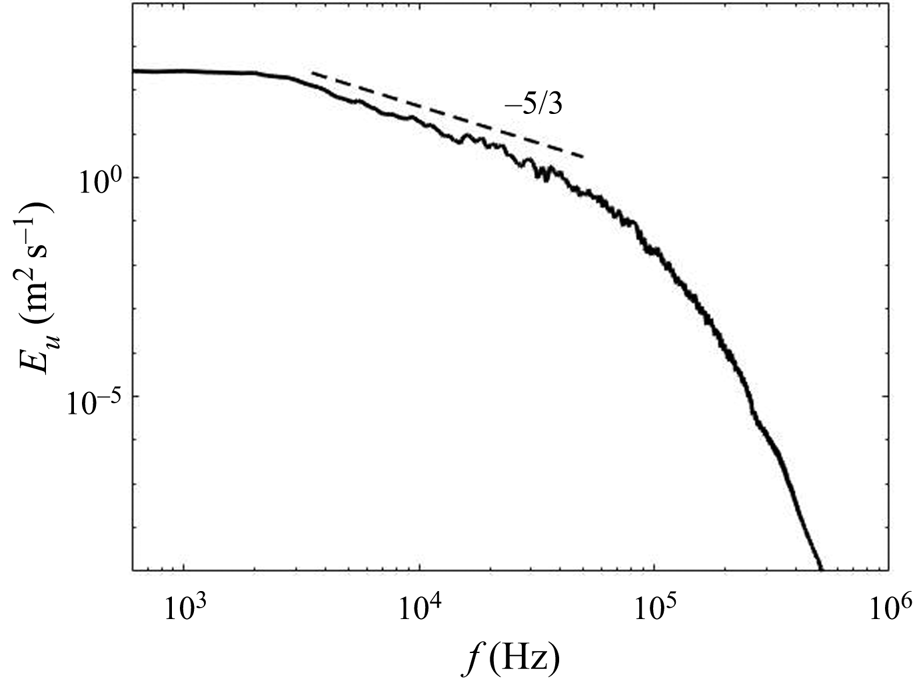
Figure 27. Energy spectrum at impingement centre [0,0,0]. The  $-$5/3 slope is indicated by the dashed line.
The resolution can also be assessed by examining the balance of turbulent kinetic energy, given by the following transport equation:
 \begin{align} &\underbrace{-U_{j} \frac{\partial}{\partial x_{j}} \left(\frac{1}{2}\langle u_{i} u_{i}\rangle\right)}_{convection} \underbrace{-\frac{\partial}{\partial x_{j}} \left(\frac{1}{\rho}\langle u_{j} p\rangle\right)}_{pressure\ work} \nonumber\\ &\quad \underbrace{-\frac{\partial}{\partial x_{j}} \left(\frac{1}{2}\langle u_{i} u_{i} u_{j} \rangle\right)}_{turbulent\ transport} \underbrace{+\frac{\partial}{\partial x_{j}} (2 \nu\langle u_{i} s_{i j}\rangle)}_{viscous\ diffusion} \underbrace{-\langle u_{i} u_{j}\rangle S_{i j}}_{production} \underbrace{-2 \nu\langle s_{i j} s_{i j}\rangle}_{dissipation} = 0. \end{align}
Here the terms represent the turbulent kinetic energy budget due to the mean convection, pressure–velocity correlation (or pressure work), turbulent transport, viscous diffusion, production and dissipation, respectively. At the statistically steady state, the sum of all these terms should be very small in a well-resolved simulation.
The terms of (B1) and their sum across the streamwise direction between the inlets are presented in figure 28. Most of the terms exhibit similar characteristics and feature peaks at or near the stream boundaries, the main exceptions being dissipation and diffusion. The evolution of the production term across the inlets is particularly strong and noticeable and, therefore, act as the main contributor to the turbulent kinetic energy budget. Its effects are balanced by the other terms. Meanwhile, turbulent transport also shares part of the contribution near the inlet and impingement centre but its sign flips at the stream boundaries, offsetting part of the production at the stream boundaries. On the other hand, the majority of the turbulent kinetic energy production is balanced by the pressure work and mean convection, whose values are mostly negative and whose peaks are collocated with the production term. While the energy dissipation is mild compared with other budget terms, it peaks at the impingement centre and is responsible for balancing the production there. Finally, the diffusion term shows only a small contribution to the balance. The sum of all budget terms in figure 28 is small and within acceptable range, as the maximum error is around  $5.5\,\%$ of the peak value of the production term. It must be emphasised that the flow in the current study is inhomogeneous in all directions. This is unlike boundary layer flow, for instance, where the homogeneous spanwise direction provides additional samples for averaging. By contrast, in the present flow the budget terms presented above are computed via temporal averaging only, and this makes it more difficult to obtain very tight balance.
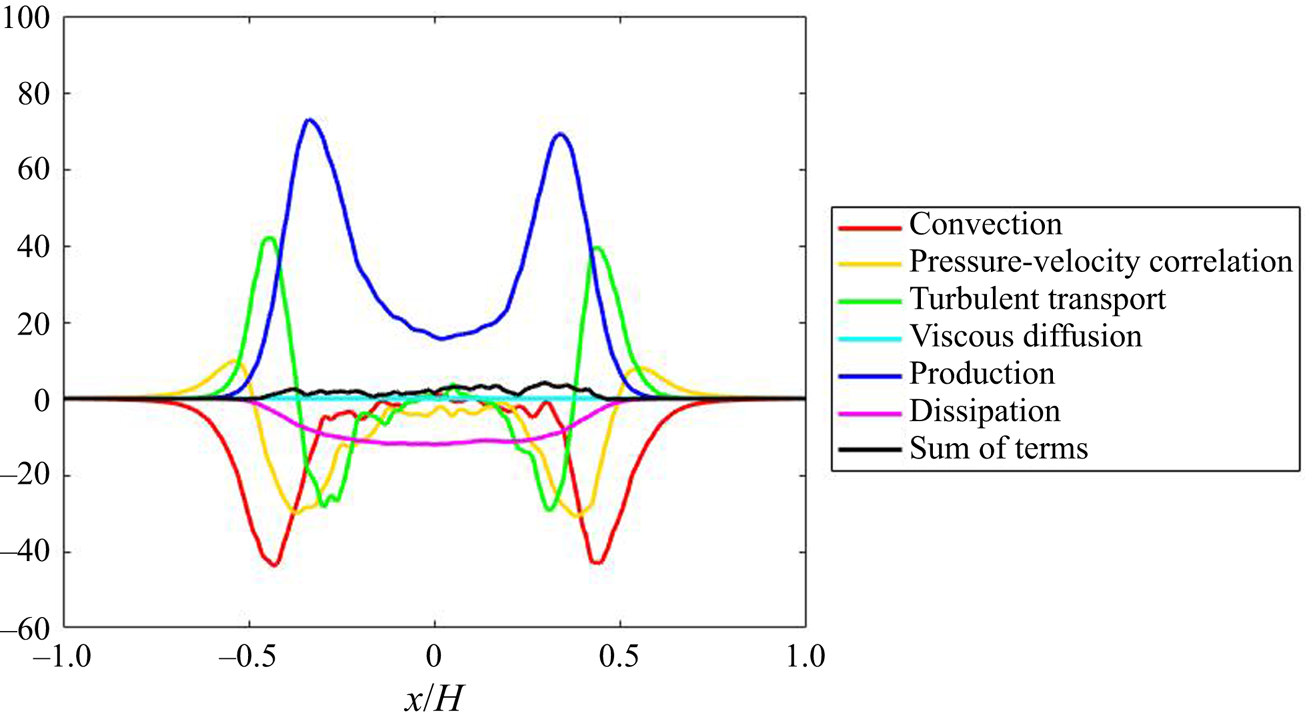
Figure 28. Turbulent kinetic energy budget terms along the inlet direction passing through the impingement centre. All terms are normalised by  $U_m^3/H$.


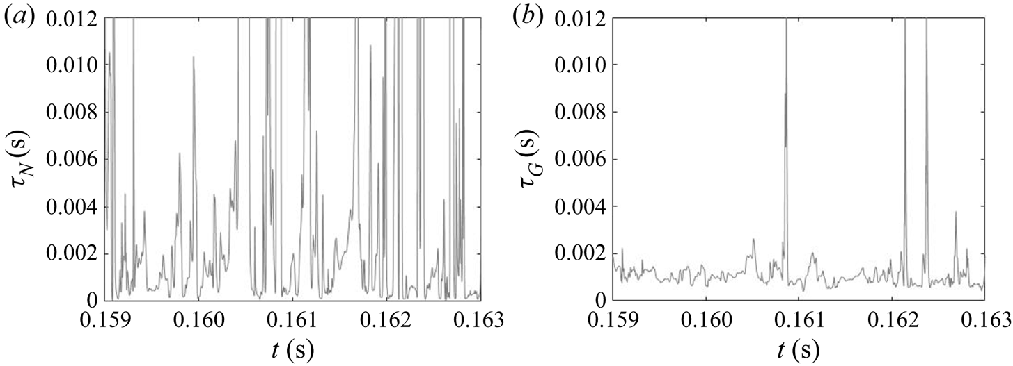


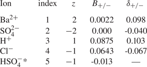


 Open access