


1. Introduction
When liquid drops are gently deposited on a hot solid surface whose temperature  $T_{w}$ is slightly above the boiling temperature $T_{b}$, the liquid boils violently resulting in rapid disappearance of the drop. However, if $T_{w}$ is increased past the Leidenfrost temperature $T_{L}$, the lifetime of the drop abruptly increases (Gottfried, Lee & Bell Reference Gottfried, Lee and Bell1966; Biance, Clanet & Quéré Reference Biance, Clanet and Quéré2003) due to the so-called Leidenfrost effect (Burton et al. Reference Burton, Sharpe, van de Veen, Franco and Nagel2012; Leidenfrost Reference Leidenfrost1756), where the drop levitates on its own vapour layer and is thus thermally shielded from the hot solid. This effect is an everyday phenomenon, seen as a water drop glides across a very hot pan, but is also crucial to numerous drop-based technologies, where the Leidenfrost effect can prevent efficient heat transfer, such as the spray cooling of high performance electronic devices (Kim Reference Kim2007) and spray combustion (Moreira, Moita & Panã Reference Moreira, Moita and Panã2010). Moreover, recent attention has been given to fascinating new topics, such as the self-propulsion of drops on ratchet surfaces (Linke et al. Reference Linke, Alemán, Melling, Taormina, Francis, Dow-Hygelund, Narayanan, Taylor and Stout2006) and hydrodynamic drag reduction (Vakarelski et al. Reference Vakarelski, Patankar, Marston, Chan and Thoroddsen2012). Fundamental studies of Leidenfrost drops, and numerous applications, are reviewed in great detail by Quéré (Reference Quéré2013) and Ling & Mudwar (Reference Ling and Mudwar2017).
At the most basic level, one would like to understand how and when the vapour film is able to retain a steady cushion for the drop and this naturally leads to a study of the geometry of the vapour film, which is complex experimentally due to its thin and almost hidden nature. In Biance et al. (Reference Biance, Clanet and Quéré2003) and Burton et al. (Reference Burton, Sharpe, van de Veen, Franco and Nagel2012) these challenges were overcome in order to experimentally record the equilibrium shapes of Leidenfrost water drops and measure the geometry of the vapour film for different drop sizes. It was demonstrated that the film thickness increases with increasing drop radii, being around  $30 - 100\,\mathrm {\mu }{\rm m}$ for drop radii of 1.6–7 mm. Using lubrication theory, and assuming an approximately uniform film, Biance et al. (Reference Biance, Clanet and Quéré2003) found good agreement with their experimental measurements, with two regimes identified based on whether the size of the drop, defined by its maximum radius $R_{max}$, is larger or smaller than the capillary length $l_{c}=(\sigma /\rho _{l}g)^{1/2}$ (dimensionlessly $\tilde {R}_{max}=R_{max}/l_{c}$, with $\tilde { }\,$ henceforth denoting dimensionless quantities), where $\sigma$ is the surface tension of the liquid–vapour interface, $g$ is gravitational acceleration and $\rho _{l}$ is the density of the liquid. Notably, for water, Burton et al. (Reference Burton, Sharpe, van de Veen, Franco and Nagel2012) showed that the vapour layer cannot be considered uniform and observed that the minimum height of this layer, at the ‘neck’, near its edge, varies from $5 - 100\,\mathrm {\mu }{\rm m}$ for drop sizes of radii 0.5–10 mm, thus motivating the development of more complex models for the film.
Variations in the profile of the vapour layer are accompanied by different drop shapes: for small drops ( $\tilde {R}_{max}<1$), surface tension dominates gravity so that the drop shape becomes quasi-spherical, with a slightly flattened base near the solid surface. Interestingly, for very small Leidenfrost drops (radii $1 - 30\,\mathrm {\mu }\mathrm {m}$), gap thicknesses actually increase with drop radius, as predicted and confirmed experimentally in Celestini, Frisch & Pomeau (Reference Celestini, Frisch and Pomeau2012), eventually leading to ‘take off’, but this regime is yet to be considered in detail computationally/theoretically.
For large drops ( $\tilde {R}_{max}>1$), gravity dominates so that a flat puddle shape is formed with a concave pocket-like geometry of the vapour layer (Burton et al. Reference Burton, Sharpe, van de Veen, Franco and Nagel2012). For a sufficiently large puddle drop, a vapour chimney forms underneath the puddle and eventually bursts at the upper surface of this drop. The onset of a chimney instability $\tilde {R}_{max} \approx 3.84$ is analytically estimated by Biance et al. (Reference Biance, Clanet and Quéré2003) by examining the Rayleigh–Taylor instability (Taylor Reference Taylor1950) of the liquid–vapour interface and then verified experimentally. Notably, Snoeijer, Brunet & Eggers (Reference Snoeijer, Brunet and Eggers2009) also found a critical radius $\tilde {R}_{max}\approx 4.0$ using a model that considered the static shapes of drops levitated by a lubricating film of air injected with constant velocity through the substrate, under isothermal conditions. For large drops, spontaneous symmetry-breaking oscillations can be observed that create the appearance of star-shaped drops (Ma, Liétor-Santos & Burton Reference Ma, Liétor-Santos and Burton2017; Brunet & Snoeijer Reference Brunet and Snoeijer2011), but these are beyond the scope of this article.
For the study of quasi-static Leidenfrost drops, Sobac et al. (Reference Sobac, Rednikov, Dorbolo and Colinet2014) proposed a theoretical model that balances the evaporation-driven viscous lubrication, hydrostatic and capillary pressures in the vapour film and matches this to a (Young–Laplace type) capillary and hydrostatic balance for the upper surface of the drop, under the assumption of axisymmetry. There are two main assumptions of the model: (i) the process is assumed to be quasi-static, with the evaporation time of the drop much longer than the viscous and thermal relaxation times in the vapour, so that the change of the drop radius can be neglected, and (ii) the liquid motion inside the drop is neglected. The theoretical predictions show very good agreement with experiments, for both the shapes of Leidenfrost water drops and the geometry of the vapour film. Despite the agreement, we will revisit the theory of Sobac et al. (Reference Sobac, Rednikov, Dorbolo and Colinet2014) in § 2, as we have seen that the original numerical solutions required reassessment (Chakraborty, Chubynsky & Sprittles Reference Chakraborty, Chubynsky and Sprittles2020); a fact which motivated our present study and led to an Erratum being published in Sobac et al. (Reference Sobac, Rednikov, Dorbolo and Colinet2021) after the authors discovered a typo in their code.
Recently, there has been interest in the dynamics of drops impacting on hot surfaces to predict the transition between the boiling and Leidenfrost regime; a question of key importance for cooling technologies (see Ling & Mudwar Reference Ling and Mudwar2017). Similarly to the static case, above the dynamic Leidenfrost temperature the drop does not touch the substrate (Tran et al. Reference Tran, Hendrik, Prosperetti and Lohse2012; Shirota et al. Reference Shirota, van Limbeek, Sun, Prosperetti and Lohse2016). Here, we will focus on developing a reliable computational model for the case of quasi-static Leidenfrost drops, with some dynamics captured for the chimney instability, and extend this in future work to study impact events.
In the aforementioned investigations, Leidenfrost drops are typically of millimetre size while the underlying vapour films are two orders of magnitude smaller, revealing a multiscale problem that makes direct computational approaches challenging. Numerical studies of the dynamics of droplets impacting on a hot surface above  $T_{L}$ have been reported using the level set/arbitrary Lagrangian Eulerian methods (Ge & Fan Reference Ge and Fan2005) and direct simulations of level set/ghost fluid methods (Villegas et al. Reference Villegas, Tanguy, Castanet, Caballina and Lemoine2017, and references therein). By using the interface capturing techniques and solving the full Navier–Stokes–Fourier equations in the whole computational domain, the drop's shape evolution and the thickness of thin vapour layer during the impact process were examined. These approaches require, on one hand, high density mesh in both the liquid and surrounding medium, especially in the thin vapour layer close to the hot surface, and on the other hand, very small time steps to produce stable and accurate numerical solutions, rendering such approaches computationally expensive and extremely challenging to produce accurate results, particularly as one approaches the transition between contact and bouncing (Chubynsky et al. Reference Chubynsky, Belousov, Lockerby and Sprittles2020).
Despite a wealth of experimental data, the computational modelling of quasi-static Leidenfrost drops over a range of parameters remains lacking from the literature. Furthermore, little research has been concerned with the interior flow and hence the effect of liquid viscosity on the process. In the present work, a robust hybrid/multiscale computational model is proposed based on coupling the lubrication approximation for the vapour flow to the Navier–Stokes equations for the flow within the drop. Numerical simulations are conducted using finite-element software and extend the work of Chubynsky et al. (Reference Chubynsky, Belousov, Lockerby and Sprittles2020), who studied the isothermal impact of a droplet on a solid surface to capture the suspension of a millimetre-sized drop by a nanoscale air film. The notable advantage of our approach is that only the liquid domain requires meshing with finite elements, with the vapour manifesting itself through the drop's boundary conditions, resulting in an efficient numerical method.
The paper is organized as follows. In §§ 2 and 3, we present two modelling approaches designed to provide insight into the Leidenfrost phenomenon: the hybrid/multiscale computational model and the theoretical framework of Sobac et al. (Reference Sobac, Rednikov, Dorbolo and Colinet2014). In § 4, we present and discuss the computational results for the various shape regimes of quasi-static Leidenfrost drops over a wide range of parameters that enable comparisons with previous experimental analyses (Biance et al. Reference Biance, Clanet and Quéré2003; Burton et al. Reference Burton, Sharpe, van de Veen, Franco and Nagel2012). Interestingly, in § 5 we discover an unexpected effect of liquid viscosity and divergence from experiments, which motivates further study. Next, in § 6, the limits of applicability of the lubrication approximation are established and a method to go beyond this is considered. Finally, in § 7, we show that our model is able to capture the dynamic chimney instability, before making concluding remarks in § 9.
2. Formulation of the computational model
Consider a Leidenfrost drop placed gently on a uniformly heated rigid horizontal surface at a constant  $T_{w}$, where $T_{w}$ is kept above $T_{L}$ ( $\gg T_{b}$), see figure 1(a). The drop levitates due to the evaporation-driven lubrication pressure which develops in the draining vapour film between the drop surface and the hot rigid wall. When the lubrication force due to vapour pressure in the gap is equal to the weight of the liquid drop, the drop is at equilibrium, as can be seen in figures 1(b) and figure 1(c). We aim to determine the quasi-static equilibrium shape of such a drop and, in particular, the underlying vapour film geometry.

Figure 1. Schematic of an axisymmetric Leidenfrost drop above an isothermal hot rigid flat surface at temperature  $T_{w}$. (a) An initially spherical drop of radius $R_0$ placed on a vapour cushion at an initial height $h_{0}$ above a heated flat surface with cylindrical coordinates ( $r,z,\theta$) shown, (b) shows an experimental image of a quasi-static Leidenfrost drop floating on a thin vapour film above a flat surface, taken from Quéré (Reference Quéré2013) and (c) a sketch of a quasi-static Leidenfrost drop levitating on a vapour layer of thickness $h(r)$. Numerical solutions of the theoretical model by Sobac et al. (Reference Sobac, Rednikov, Dorbolo and Colinet2014) (see § 2) are obtained by patching the solution for the upper surface of the drop to that for the lower surface bordering the lubrication vapour layer, at $r=R_{p}$. The image shows the maximum droplet radius $R_{max}$, the radius of the neck $R_{neck}$ and the height of the neck measured from the solid surface (minimum vapour film thickness) $h_{neck}$. The evaporation mass flux across the liquid–vapour interface is denoted by $j$.
$j$.
We consider an axisymmetric problem, an assumption which is discussed later, described in the cylindrical coordinate system  $(r, z, \theta )$, where $r$ is the radial coordinate, $z$ is the axial coordinate measured in the opposite direction of gravity and the problem is considered to be independent of the azimuthal coordinate $\theta$. As shown in figure 1, $z=0$ and $r=0$ represent the solid wall and the axis of symmetry, respectively. Even though the liquid and vapour properties are temperature dependent, in this study, for simplicity, we assume they can be approximately evaluated at the boiling temperature $T_{b}$ and at the mean temperature $T_{m}=(({T_{w}+T_{b}})/{2}$) between the wall and liquid, respectively, similar to Sobac et al. (Reference Sobac, Rednikov, Dorbolo and Colinet2014).
In this section, we formulate our computational model and then, in the next section, show how this relates to the simplified theoretical model of Sobac et al. (Reference Sobac, Rednikov, Dorbolo and Colinet2014). Our approach, which naturally extends to the consideration of dynamic processes, is to start with an initially spherical liquid drop of radius  $R_{0}$ which is released from rest above a solid at a height $h_{0}=0.1R_{0}$, as shown in figure 1(a), falls due to gravity and then evolves dynamically in time towards a quasi-static shape.
2.1. Liquid flow
The flow of liquid inside the drop is governed by the isothermal incompressible Navier–Stokes equations, with incompressibility
 \begin{equation} \frac{1}{r}\frac{\partial (ru_{l})}{\partial r}+\frac{\partial w_{l}}{\partial z}=0, \end{equation}
and the momentum equations
 \begin{gather} \rho_{l}\left(\frac{\partial{u_{l}}}{\partial t} + u_{l}\frac{\partial{u_{l}}}{\partial{r}}+w_{l}\frac{\partial{u_{l}}}{\partial{z}}\right) ={-} \frac{\partial{p_{l}}}{\partial r} + \mu_{l} \left(\frac{\partial^{2}u_{l}}{\partial r^{2}}+\frac{1}{r}\frac{\partial u_{l}}{\partial r}+\frac{\partial^{2}u_{l}}{\partial z^{2}}-\frac{u_{l}}{r^{2}}\right), \end{gather}
 \begin{gather} \rho_{l}\left(\frac{\partial{w_{l}}}{\partial t} + u_{l}\frac{\partial{w_{l}}}{\partial{r}}+w_{l}\frac{\partial{w_{l}}}{\partial{z}}\right) ={-} \frac{\partial{p_{l}}}{\partial z} + \mu_{l} \left(\frac{\partial^{2}w_{l}}{\partial r^{2}}+\frac{1}{r}\frac{\partial w_{l}}{\partial r}+\frac{\partial^{2}w_{l}}{\partial z^{2}}\right)-\rho_{l}{g}, \end{gather}
where henceforth a subscript  $l$ denotes the liquid phase and $v$ will denote the vapour. Here, $\rho$ will represent densities; $\mu$ dynamic viscosities; $u$ and $w$ are velocity components in the $r$ and $z$ directions; $p$ is the pressure; and $t$ is the time.
2.2. Vapour flow
In the vapour film we develop a lubrication model, with height  $h(r,t)$ considered slowly varying ( ${\partial h}/{\partial r}\ll 1$) and small compared with the drop size $R_{max}$ ( $\epsilon =h/R_{max} \ll 1$) in those parts of the film that contribute significantly to the pressure drop in the film and vapour generation. In addition, we neglect the influence of gravity in the vapour layer and consider inertial forces negligible compared with viscous ones, for which we need $\epsilon Re_{v} \ll 1$ (Aursand, Davis & Ytrehus Reference Aursand, Davis and Ytrehus2018), where the Reynolds number of the thin vapour layer is defined as $Re_{v}=\rho _{v}h^{3}\vert \boldsymbol {\nabla } p_{v}\vert /\mu ^{2}_{v}$ (Biance et al. Reference Biance, Clanet and Quéré2003; Celestini et al. Reference Celestini, Frisch and Pomeau2012; Aursand et al. Reference Aursand, Davis and Ytrehus2018). This establishes the use of lubrication theory in the vapour film (Biance et al. Reference Biance, Clanet and Quéré2003; Sobac et al. Reference Sobac, Rednikov, Dorbolo and Colinet2014; Aursand et al. Reference Aursand, Davis and Ytrehus2018), with incompressibility unchanged
 \begin{equation} \frac{1}{r}\frac{\partial (ru_{v})}{\partial r}+\frac{\partial w_{v}}{\partial z}=0, \end{equation}
and the momentum equations simplifying to
 \begin{equation} \frac{\partial p_{v}}{\partial r}= \mu_{v}\frac{\partial^{2} u_{v}}{\partial z^{2}} \quad \mathrm{and}\quad \frac{\partial p_{v}}{\partial z}=0. \end{equation}
 The velocity component tangent to the interface ( $z=h(r,t)$) is assumed continuous across it, so that $u_{v,\varGamma }=u_{l,\varGamma }\equiv u_{\varGamma }$, where $\varGamma$ indicates a surface property of the liquid–vapour interface and subscripts $v,\varGamma$ and $l,\varGamma$ refer to bulk properties at the interface. By integrating equation (2.5a,b) with the boundary conditions $u_{v}(z=0)=0$ at the solid wall and $u_{v}(z=h(r,t))=u_{\varGamma }$ at the drop surface, the local radial velocity profile in the lubricating film is obtained as
 \begin{equation} u_{v}(r,z,t)= \frac{1}{2\mu_{v}}\frac{\partial p_{v}(r,t)}{\partial r}\{z^{2}-zh(r,t)\} + u_{\varGamma}(r,t)\frac{z}{h(r,t)}. \end{equation}
This shows that the radial velocity profile underneath the drop is expressed by the superposition of two components, a Poiseuille flow (pressure-driven) component with an immobile interface and a Couette flow driven by the interface's tangential velocity with no pressure gradient.
In the Leidenfrost phenomenon, heat transfer and evaporation both take place in the region of the vapour film. Under the considered lubrication approximation, the effects of convective heat transfer are negligible compared with thermal conduction when  $\epsilon Re_{v} Pr_{v}\ll 1$, where the Prandtl number is $Pr_{v}=\mu _{v}c_{p,v}/k_{v}$ (for water vapour $Pr_{v}\approx 0.95$ at $T_{m}=200\,^{\circ }\mathrm {C}$), and $k_{v}$ and $c_{p,v}$ are thermal conductivity and specific heat capacity (see Aursand et al. Reference Aursand, Davis and Ytrehus2018) . Hence, in the lubrication approximation the energy conservation equation simplifies to
 \begin{equation} \frac{\partial^{2} T_{v}}{\partial z^{2}}=0, \end{equation}
which indicates that the temperature across the vapour film varies linearly between the solid surface temperature  $T_{v}\arrowvert _{z=0}=T_{w}$ and the liquid–vapour interface temperature $T_{v}\arrowvert _{z=h}=T_{b}$.
Let the rate of change of the vapour film height in the frame of reference moving horizontally with speed  $u_{\varGamma }$ be $w_{\varGamma }$. Then in the laboratory frame
 \begin{equation} \frac{\partial h}{\partial t}=w_{\varGamma}-u_{\varGamma}\frac{\partial h}{\partial r}. \end{equation}
Without evaporation, the usual kinematic boundary conditions then give  $w_{\varGamma }=w_{l,\varGamma }=w_{v,\varGamma }$, where $w_{l,\varGamma }$ and $w_{v,\varGamma }$ are the vertical liquid and vapour velocities at the interface, respectively. In our case, the heat transferred by conduction from the hot solid to the drop is used for evaporative vapour generation at the liquid–vapour interface (as the temperature in the liquid is assumed fixed at its boiling point, so there is no heat flux into it). In this case, mass and energy conservation at $z=h$ yield (keeping in mind that the interface is nearly horizontal)
 \begin{equation} \rho_{v}(w_{v,\varGamma}-w_{\varGamma})=\rho_{l}(w_{l,\varGamma}-w_{\varGamma})={-}j,\quad \mathrm{and}\quad q_{v}=jL, \end{equation}
where  $j$ is the evaporative mass flux through the liquid–vapour interface and $L$ is the latent heat of evaporation. Equation (2.9) implies that the vertical velocities undergo a jump across the interface due to evaporation.
Since  $\eta =\rho _{v}/\rho _{l} \sim 10^{-3}$, (2.9) implies that $w_{v,\varGamma }-w_{\varGamma }$ is very large compared with $w_{l,\varGamma }-w_{\varGamma }$; thus, we can assume $w_{\varGamma }=w_{l,\varGamma }$. Furthermore, the low density ratio $\eta$ establishes that the timescales for viscous and thermal diffusion in the vapour film are very small compared with the liquid in the drop, which also marks a quasi-static process in this Leidenfrost phenomenon. In (2.9), the heat flux $q_{v}$ is modelled by Fourier's law expressed as
 \begin{equation} q_{v}={-}k_{v}\left(\frac{\partial T}{\partial z}\right){\vert}_{z=h}=\frac{k_{v}\Delta T}{h}, \end{equation}
where  $\Delta T=T_w-T_b$. Hence, (2.9) with (2.8) at $z=h$ can be rewritten as
 \begin{equation} w_{v,\varGamma}=\frac{\partial h}{\partial t}+u_{\varGamma}\frac{\partial h}{\partial r}-\frac{k_{v}\Delta T}{L\rho_{v}h}. \end{equation}
By substituting (2.6) into (2.4) and integrating equation (2.4) over the film thickness in the vertical direction with boundary conditions  $w_{v}\arrowvert _{z=0}=0$ and $w_{v}\arrowvert _{z=h}=w_{v,\varGamma }$ (obtained from (2.11)), and applying the Leibniz integral rule, we get
 \begin{equation} \frac{1}{r}\frac{\partial}{\partial r}\left \{r\left(-\frac{h^{3}}{12\mu_{v}}\frac{\partial p_{v}}{\partial r} + u_{\varGamma}\frac{h}{2}\right) \right \}+\frac{\partial h}{\partial t}-\frac{k_{v}\Delta T}{L\rho_{v}h}=0. \end{equation}
Note that, in regions where the lubrication assumptions are not valid,  $h$ is large, the last (evaporation) term vanishes, so the expression in braces is constant and then $\partial p_v/\partial r\approx 0$, which is still correct, so the equation remains valid. From (2.12), one readily obtains the pressure distribution $p_{v}(r,t)$ in the film expressed as a differential equation along the liquid–vapour interface
 \begin{equation} \frac{\partial^{2}p_{v}}{\partial r^{2}}+\frac{\partial}{\partial r}\{\ln{(rh^{3})}\}\frac{\partial p_{v}}{\partial r}=\frac{6\mu_{v}}{rh^{3}}\left \{{-}2r\frac{k_{v}\Delta T}{L\rho_{v}h}+\frac{\partial}{\partial r}\left(rhu_{\varGamma}\right )+2r\frac{\partial h}{\partial t}\right \}. \end{equation}
The corresponding boundary conditions are given by
 \begin{equation} \frac{\partial p_{v}}{\partial r}{\bigg \vert}_{r=0}=0\quad \mathrm{and}\quad p_{v}\arrowvert_{r=r_{o}}=p_{o}. \end{equation}
Here,  $r_{o}$ is defined at the boundary of the vapour film where $p_{o}=0$ is equal to the atmospheric pressure (i.e. pressures are measured relative to their atmospheric value). The exact choice of $r_{o}$ is discussed below. Finally, in the lubrication approximation, the shear stress on the drop surface is given by $\tau _{v}(r,t)=\mu _{v}(\left.{\partial u_{v}}/{\partial z}\right |)_{z=h}$. This leads to
 \begin{equation} \tau_{v}=\frac{h}{2}\left(\frac{\partial p_{v}}{\partial r}\right)+\mu_{v}\frac{u_{\varGamma}}{h} \end{equation}
with, as expected, terms from both Poiseuille and Couette components.
2.3. Boundary conditions
In order to solve the Navier–Stokes equations (2.1)–(2.3), we need the free surface boundary conditions: normal and shear stresses are enforced on the entire drop surface. For this purpose, the drop surface is divided into two parts, as considered also in the theory of Sobac et al. (Reference Sobac, Rednikov, Dorbolo and Colinet2014), separated at  $r=r_{o}$. The top of the drop (part 1) is modelled conventionally with the ambient pressure equal to the atmospheric pressure ( $p_{o}=0$), the normal stress is equal to the Laplace pressure, and the shear stress is zero. The bottom of the drop (part 2), adjacent to the vapour layer, has (i) the normal stress set to the sum of Laplace pressure and the lubrication pressure $p_{v}(r,t)$, where $p_{v}(r,t)$ is obtained by solving (2.13) and (ii) the shear stress $\tau _{v}(r,t)$ given by (2.15). Note that $p_{v}(r,t)$ and $\tau _{v}(r,t)$ depend on the radial velocity of the liquid ( $u_{\varGamma }=u_{l,\varGamma }$) at the free surface, and $\partial h/\partial t$ in (2.8) depends on the vertical velocity of the liquid ( $w_{\varGamma }=w_{l,\varGamma }$) at the interface, which are obtained simultaneously by solving the Navier–Stokes equations for the drop. We choose $r_{o}$ to be at the maximum radial extent of the drop surface where the vapour pressure is nearly equal to the atmospheric pressure. The computed results are insensitive to the exact value of $r_{o}$ providing at that point the value of $h$ is much larger than that in the vapour layer at its thinnest point; see the supplemental material of Chubynsky et al. (Reference Chubynsky, Belousov, Lockerby and Sprittles2020) for more details. Note also that the conventional kinematic boundary condition for the evolution of the free surface of the drop in terms of the liquid velocity at the surface applies everywhere on the surface, since in parts of the surface where evaporation is not negligible, $u_{l,\varGamma }=u_{\varGamma }$ and $w_{l,\varGamma }=w_{\varGamma }$ is still assumed.
2.4. Computational implementation
Our hybrid/multiscale computational model is solved in Comsol Multiphysics (COMSOL Ltd., Cambridge, UK; version 5.4) using finite elements, as described in Appendix A.
3. Theoretical model
This section reviews the theoretical framework proposed by Sobac et al. (Reference Sobac, Rednikov, Dorbolo and Colinet2014) and discusses its connections to the computational model just derived. Further details of the numerical implementation are provided in Appendix A. As previously, the surface of an axisymmetric Leidenfrost drop at equilibrium is divided into two parts, separated by a patching point ( $R_{p}, h_{p}$), with the upper and lower drop surfaces treated differently, as shown in figure 1(c). We choose the patching point to lie at the position where ${\rm d}\tilde {z}/{\rm d}\tilde {r}=1$. This is different from the choice we have made in our computational model (see § 2); thus, agreement between the two models will also indicate insensitivity to the choice of the patching point. The upper surface of the drop is determined from the Young–Laplace equation and the lower surface is, in addition, affected by a lubrication pressure from the thin vapour layer, with the two solutions matched at the patching point in order to predict the equilibrium shape of the drop.
First, the shape of the upper surface of the drop at equilibrium is governed by a balance between the interfacial capillary pressure and hydrostatic pressure variations in the liquid,
 \begin{equation} \sigma\kappa-\rho_{l}g z_1=\sigma\kappa_{apex}, \end{equation}
where  $z_1=z-z_{top}$ is the vertical coordinate measured from the apex of the drop ( $z=z_{top}$) and $\kappa _{apex}$ is the curvature of the drop surface at the apex. This equilibrium condition neglects internal flow in the drop, which is taken into account in our computational model. In dimensionless form (with respect to the capillary length),
 \begin{equation} \tilde \kappa =\tilde{z}_1 + \tilde{\kappa}_{apex}. \end{equation}
Given  $\tilde {\kappa }_{apex}$, (3.2) can be solved to obtain the shape of the upper surface, in the form of the dependences ${\tilde {z}_1}({\tilde {s}})$ and ${\tilde {r}}({\tilde {s}})$, where $\tilde {s}$ is the arc length measured from the apex (Duchemin, Lister & Lange Reference Duchemin, Lister and Lange2005). Rather than specifying the size of the drop $\tilde {R}_{max}$, it is more convenient to choose ${\tilde {\kappa }}_{apex}$ instead and $\tilde {R}_{max}$ is then found from the solution. Note that at this point $\tilde {z}_{top}$ remains unknown, in other words, the shape is determined up to a vertical shift.
Second, for the lower surface we include the vapour pressure, and then the equilibrium condition (again neglecting the liquid flow) is
 \begin{equation} p_v+\rho_l gh+\sigma\kappa=\mathrm{const.} \end{equation}
We next use (2.12), where we again neglect the liquid flow and therefore  $u_{\varGamma }$, which gives
 \begin{equation} \frac{\partial h}{\partial t}=\frac{k_{v}\Delta T}{L\rho_{v}h}-\frac{1}{r}\frac{\partial}{\partial r}\left \{r\left(-\frac{h^{3}}{12\mu_{v}}\frac{\partial p_{v}}{\partial r}\right) \right \}. \end{equation}
Using (3.3) to eliminate  $p_v$ and switching to dimensionless variables, we get
 \begin{equation} \frac{\partial \tilde{h}}{\partial \tilde{t}}=\frac{E}{\tilde{h}}-\frac{1}{12\tilde{r}}\frac{\partial}{\partial \tilde{r}}\left[\tilde{r} \tilde{h}^{3}\frac{\partial}{\partial \tilde{r}}\left(\tilde{h}+\tilde{\kappa} \right)\right], \end{equation}
where  ${\tilde {t}}=t/t_c$ with $t_{c}=\mu _{v}l_{c}/\sigma$. Note that (3.5) does not describe the true time evolution of the film thickness, since (3.3) is only valid in equilibrium; in fact, true dynamics depends on liquid viscosity and becomes infinitely slow as $\mu _l\to \infty$. However, the steady state of (3.5) is correct (indeed, putting $\partial \tilde {h}/\partial \tilde {t}=0$ turns it into the main equation of the theory of Sobac et al. Reference Sobac, Rednikov, Dorbolo and Colinet2014); the time derivative is retained for computational reasons and the steady-state profile is obtained as a result of time evolution in the long-time limit. It can be seen that (3.5) depends on a single dimensionless parameter
 \begin{equation} E=\frac{k_{v}\mu_{v}\Delta T}{\sigma L\rho_{v}l_{c}}, \end{equation}
which is the (dimensionless) evaporation number. In most cases, we find the condition  $E \ll 1$ which represents slow evaporation, corroborating the consideration of a quasi-static process. Note that the exact expression for the curvature, not assuming the slow variation of film thickness,
 \begin{equation} \tilde{\kappa}=\frac{\dfrac{\partial^{2} \tilde{h}}{\partial \tilde{r}^{2}}}{\left [1+\left (\dfrac{\partial \tilde{h}}{\partial \tilde{r}} \right)^{2} \right]^{3/2}}+\dfrac{\dfrac{\partial \tilde{h}}{\partial \tilde{r}}}{\tilde{r} \left [1+\left (\dfrac{\partial \tilde{h}}{\partial \tilde{r}} \right)^{2} \right]^{1/2}} \end{equation}
is used in (3.5), which makes that equation valid in parts of the surface where the lubrication approximation is not valid (but the terms calculated using that approximation are negligible).
Equation (3.5) is fourth order in  $\tilde {r}$ and therefore requires four boundary conditions: ${\rm d}\tilde {h}/{\rm d}\tilde {r}={\rm d}{\tilde {\kappa }}/{\rm d}{\tilde {r}}=0$ at the axis of symmetry $\tilde {r}=0$, and matching of ${\rm d}\tilde {h}/{\rm d}\tilde {r}$ and $\tilde {\kappa }$ at $\tilde {r}=\tilde {R}_{p}$ with the corresponding values obtained from the upper surface of the drop. After obtaining a steady-state solution, the continuity of $\tilde {h}(\tilde {r})$ itself simply amounts to translating vertically the upper surface of the drop, thus determining $\tilde {z}_{top}$ and revealing the complete equilibrium shape of the drop.
Whilst this formulation still requires a numerical solution, we refer to it as the ‘theoretical model’ or ‘theoretical solutions’ to distinguish it from the solutions to our computational model, which additionally solve for the internal flow via the Navier–Stokes equations.
To summarize, the theoretical model of Sobac et al. (Reference Sobac, Rednikov, Dorbolo and Colinet2014) can be obtained from our computational model by neglecting the flow inside the drop and thus the results of the models are expected to coincide when this flow is negligible, i.e. when the liquid viscosity  $\mu _l$ is large.
4. Leidenfrost drop shapes and identification of regimes
We are now in a position to compare our computational model with experimental analyses conducted on water drops and utilize it to establish the limits of applicability of the theoretical model. As described, the theoretical model neglects flow within the droplet and so to imitate this state with our computational model we align all parameters with those used in experiments (i.e. for water drops of a given size on a surface at a given temperature) with the exception of liquid viscosity which is set at a high value. This has the effect of ‘turning off’ the connection between the internal flow and the vapour film dynamics. The effect of internal flow can then be isolated and is investigated in § 5.
4.1. Shapes of Leidenfrost drops
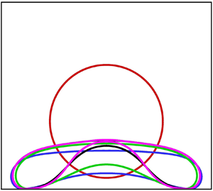
Figure 2 shows the shapes of quasi-static Leidenfrost drops at equilibrium predicted by our computational model for four different sizes  $\tilde {R}_{max}=0.26, 0.41, 2.69, 3.72$ at a fixed evaporation number $E=6.26\times 10^{-7}$ (all parameters are given in the caption) of a high-viscosity liquid ( $\mu _{l}=0.3\,\mathrm {Pa}\,\mathrm {s}$). Superimposed are the theoretical solutions showing excellent agreement is obtained. Four distinct regimes are observed upon increasing the drop size:
(i) Dimpleless quasi-spherical drop – where the drop is approximately spherical as $\tilde {R}_{max}<1$ and the curvature does not change sign at the bottom of the drop, seen in figure 2(a) for $\tilde {R}_{max}=0.26$.
(ii) Dimpled quasi-spherical drop – where the drop is approximately spherical as
$\tilde {R}_{max}<1$ but now a vapour pocket is formed under the drop, which is seen in figure 2(b) at $\tilde {R}_{max}=0.41$.(iii) Puddle-like drop – where gravity flattens the drop as
$\tilde {R}_{max}>1$, as seen in figure 2(c) for $\tilde {R}_{max}=2.69$.(iv) Chimney instability – where stable quasi-static shapes no longer exist. In figure 2(d) we show a case
$\tilde {R}_{max}=3.72$ close to where this instability occurs.


Figure 2. Comparison of the computational (black line) and theoretical (yellow dashed line) equilibrium shapes of Leidenfrost drops at  $T_{b}=100\,^{\circ }\mathrm {C}$ above a hot rigid surface at $T_{w}=300\,^{\circ }\mathrm {C}$ for (a) $\tilde {R}_{max}=0.26$, (b) $\tilde {R}_{max}=0.41$, (c) $\tilde {R}_{max}=2.69$ and (d) $\tilde {R}_{max}=3.72$. At $T_{m}=200\,^{\circ }\mathrm {C}$, the input parameters (Biance et al. Reference Biance, Clanet and Quéré2003) are $\rho _{v}=0.5\,\mathrm {kg}\,\mathrm {m}^{-3}$, $\mu _{v}=1.63\times 10^{-5}\,\mathrm {Pa}\,\mathrm {s}$, $k_{v}=0.032\,\mathrm {W}\,\mathrm {m}^{-1}\,\mathrm {K}^{-1}$ and the latent heat of evaporation $L=2.26\times 10^{6}\,\mathrm {J}\,\mathrm {kg}^{-1}$ at $T_{b}=100\,^{\circ }\mathrm {C}$ and thus the calculated value of evaporation number $E=6.259\times 10^{-7}$. Here, simulations are carried out for a higher-than-water dynamic liquid viscosity of $\mu _{l}=0.3\,\mathrm {Pa}\,\mathrm {s}$.
It is noticeable from figure 2(b–d) that the region of the deformed drop adjacent to the steady vapour film takes a dimple shape (an approximately parabolic shape with curvature opposite to that of the undeformed sphere), with a maximum vapour film thickness  $h_{centre}$ at the centre of the vapour layer $r=0$ and a minimum film thickness $h_{neck}$ defining the neck $r=R_{neck}$; see also figure 1. This dimpled regime is well known, and was first observed experimentally discovered for Leidenfrost droplets in Burton et al. (Reference Burton, Sharpe, van de Veen, Franco and Nagel2012), having been theoretically predicted for a drop suspended by an upward air flow from a permeable solid in Duchemin et al. (Reference Duchemin, Lister and Lange2005) for curved substrates and Snoeijer et al. (Reference Snoeijer, Brunet and Eggers2009) for flat ones, and having been seen in a variety of other drop/gas-film interactions, such as drop impact (Chandra & Avedisian Reference Chandra and Avedisian1991; Thoroddsen, Etoh & Takehara Reference Thoroddsen, Etoh and Takehara2003). In contrast, the dimpleless regime in figure 2(a), also commented on in Sobac et al. (Reference Sobac, Rednikov, Dorbolo and Colinet2021), is a new phenomenon.
4.2. Geometry of the vapour film
To enable a comparison with the experimental results in Biance et al. (Reference Biance, Clanet and Quéré2003) and Burton et al. (Reference Burton, Sharpe, van de Veen, Franco and Nagel2012), we consider the geometry of the vapour film using the parameters from these experiments (with the exception of liquid viscosity). In particular, in figure 3 we present the dependence of the vapour film thickness at the neck  $h_{neck}$, the difference in vapour film thickness $\Delta h=h_{centre}-h_{neck}$ and the film's neck radius $R_{neck}$ on the drop size $R_{max}$ varying over the range of $0.65\,\mathrm {mm} \le R_{max} \lesssim 10.0\,\mathrm {mm}$. This is done for two different wall temperatures $T_{w}=300\,^{\circ }\mathrm {C}\ \mathrm {and}\ 370\,^{\circ }\mathrm {C}$, corresponding to $E=6.259\times 10^{-7}\ \mathrm {and}\ 1.01\times 10^{-6}$, at high liquid viscosity $\mu _{l}=0.3\,\mathrm {Pa}\,\mathrm {s}$. In general, it is observed that the computed $h_{neck}$, $\Delta h$ and $R_{neck}$ all increase with $R_{max}$; $\Delta h$ and $R_{neck}$ are nearly independent of wall temperature $T_{w}$; and $h_{neck}$ somewhat increases with $T_{w}$.

Figure 3. Comparison of the computational model with experiments for the geometry of the vapour layer underneath a Leidenfrost drop. (a) The vapour film thickness at the neck  $h_{neck}$ vs the drop size $R_{max}$, (b) the difference in the vapour film thickness $\Delta h=h_{centre}-h_{neck}$ as a function of $R_{max}$ and (c) the neck radius $R_{neck}$ vs $R_{max}$, see figures 1 and 2. The solid line represents the results of our computational model for $T_{w}=300\,^{\circ }\mathrm {C}\ \mathrm {and} 370\,^{\circ }\mathrm {C}$ and $\mu _{l}=0.3\,\mathrm {Pa}\,\mathrm {s}$, compared with the symbols corresponding to the experimental data reported by Burton et al. (Reference Burton, Sharpe, van de Veen, Franco and Nagel2012) for $T_{w}=245\,^{\circ }\mathrm {C}, 320\,^{\circ }\mathrm {C}\ \mathrm {and}\ 370^{\circ }\mathrm {C}$ (for water drops), the dashed-dot lines are the solutions of the theoretical model; the vertical dotted line denotes the computed critical value of $R_{max,DL-D}$ below which ‘dimpleless’ (DL) regime with a nearly spherical drop shape can be seen, with the ‘dimpled’ (D) regime for higher $R_{max}$. In addition, the experimental data of Biance et al. (Reference Biance, Clanet and Quéré2003) for $h_{neck}$ (filled circle symbols) at $T_{w}=300\,^{\circ }\mathrm {C}$ (for water) are plotted in (a).
Notably, the computational model was able to identify differences with the solutions presented in Sobac et al. (Reference Sobac, Rednikov, Dorbolo and Colinet2014) that, upon seeing our results (in Chakraborty et al. Reference Chakraborty, Chubynsky and Sprittles2020), the authors were able to correct in Sobac et al. (Reference Sobac, Rednikov, Dorbolo and Colinet2021). In particular, for smaller values of  $R_{max}$, where the dimpleless regime sits, the original solution of the theoretical model from Sobac et al. (Reference Sobac, Rednikov, Dorbolo and Colinet2014) diverges from the corrected solution (Sobac et al. Reference Sobac, Rednikov, Dorbolo and Colinet2021).
In figure 3, we compare the result of our computational model with experiments and the theoretical model. Results for  $\Delta h$ and $R_{neck}$ show very good agreement with the experimental data of Burton et al. (Reference Burton, Sharpe, van de Veen, Franco and Nagel2012) when $R_{max}\gtrsim 1.0\,\mathrm {mm}$. For smaller values of $R_{max}$, we see discrepancies appearing between our predictions and experiments. This is worthy of further attention and could be caused by increased scatter from the indirect measurements as the film height shrinks (Burton et al. Reference Burton, Sharpe, van de Veen, Franco and Nagel2012) or due to the motion of the drop laterally (Bouillant et al. Reference Bouillant, Mouterde, Bourrianne, Lagarde, Clanet and Quéré2018). Qualitatively, it is noteworthy that experimental data for $\Delta h$ for 245 and $320\,^{\circ }\mathrm {C}$ rapidly decrease with decreasing $R_{max}$, indicating an approach to the dimple-less regime we have predicted. However, in figure 3(a) data for $h_{neck}$ from the experiment of Burton et al. (Reference Burton, Sharpe, van de Veen, Franco and Nagel2012) go into the dimpleless regime, where the neck no longer exists in our computational model; the reason for this discrepancy remains unclear. Furthermore, our results in figure 3(a) show less good agreement with experimental data of Biance et al. (Reference Biance, Clanet and Quéré2003) for minimum film thickness $h_{neck}$, at $T_w = 300\,^{\circ }\mathrm {C}$, particularly for larger drop sizes. The reason is not clearly understood, but a probable explanation is that Biance et al. (Reference Biance, Clanet and Quéré2003) measure an effective vapour film thickness, and never actually discuss the height at the neck, and it is inferred here, as in Sobac et al. (Reference Sobac, Rednikov, Dorbolo and Colinet2014), that this value is closely related to the local measurement $h_{neck}$.
To further study the geometry of the vapour film and establish how/if the liquid viscosity influences it, in figure 4 we compute the dimensionless vapour film thickness at the centre  $\tilde {h}_{centre}=h_{centre}/l_{c}$ and at the neck $\tilde {h}_{neck}=h_{neck}/l_{c}$ as a function of the dimensionless drop size $0.0016 \le \tilde {R}_{max} \lesssim 4.0$ for fixed $E=1.01\times 10^{-6}$ ( $T_{w}=370\,^{\circ }\mathrm {C}$). In this case, which is used in many forthcoming calculations, the vapour density is $\rho _v=0.47\,{\rm kg}\,{\rm m}^{-3}$, its viscosity $\mu _v=1.70\times 10^{-5}\,{\rm Pa}\,{\rm s}$, its conductivity is $k_v=0.0347\,{\rm Wm}^{-1}\,{\rm K}^{-1}$ and the latent heat of vaporization is $L=2.26\times 10^{6}\,{\rm J}\,{\rm kg}^{-1}$. Calculations are done using both the dynamic viscosity of water $\mu_{l,water}=0.00034\,\mathrm {Pa}\,\mathrm {s}$ at $T_{b}=100\,^{\circ }\mathrm {C}$ and the high dynamic viscosity $\mu _{l,high}=0.3\,\mathrm {Pa}\,\mathrm {s}$ (used in previous results). The theoretical model's results are also plotted and have no dependence on internal flow and hence liquid viscosity. These are both compared with experimental data for Leidenfrost water drops (Burton et al. Reference Burton, Sharpe, van de Veen, Franco and Nagel2012) and are now considered by regime.

Figure 4. The vapour film thickness at the centre  $\tilde {h}_{centre}$ and at the neck $\tilde {h}_{neck}$ vs the drop size $\tilde {R}_{max}$ for $E=1.01\times 10^{-6}$ ( $T_{w}=370\,^{\circ }\mathrm {C}$). The red and blue solid/dashed lines correspond to the results of the computational model for $\mu _{l,water}=0.00034\, \mathrm {Pa}\,\mathrm {s}$ (water) and $\mu _{l,high}=0.3\, \mathrm {Pa}\,\mathrm {s}$ (high viscosity), respectively, compared with the theoretical solution. Regimes marked on the plot correspond to (i) dimpleless quasi-spherical drops, (ii) dimpled quasi-spherical drops, (iii) dimpled puddles and (iv) chimney instabilities. The experimental data for $\tilde {h}_{centre}$ are obtained from the data for $\tilde {h}_{centre}-\tilde {h}_{neck}$ and $\tilde {h}_{neck}$ given by Burton et al. (Reference Burton, Sharpe, van de Veen, Franco and Nagel2012).
4.2.1. Dimpleless quasi-spherical drops: $\tilde {R}_{max} < \tilde {R}_{max,DL-D}=0.3$

In this regime, figure 4 shows that for both viscosities computational and theoretical curves for  $\tilde {h}_{centre}$ merge with those for $\tilde {h}_{neck}$ indicating a dimpleless regime. Interestingly, in this regime, there is non-monotonic behaviour, with both heights initially decreasing with smaller $\tilde {R}_{max}$, reaching a minimum at $\tilde {R}_{max,hmin} \approx 0.14$, after which film heights increase, in qualitative agreement with the experimental discoveries made in Celestini et al. (Reference Celestini, Frisch and Pomeau2012). Computational and theoretical results are in excellent agreement above the minima ( $0.14 \le \tilde {R}_{max} \le 0.3$) but discrepancies appear below it, where the accuracy of the lubrication approximation is reduced as the film height becomes comparable to the drop size; going beyond the lubrication approximation will be discussed in § 6. Notably, it can be observed (not shown here) that our results of $\tilde {h}_{min}$ and $\tilde {R}_{max,hmin}$ are only relatively weakly sensitive to the variation in the evaporation number $E$ or $T_{w}$.
4.2.2. Dimpled quasi-spherical drops: $\tilde {R}_{max,DL-D}<\tilde {R}_{max} <1$

Here, the dimpleless regime gives way to the well-known dimpled regime with figure 4 showing that film heights increase with  $\tilde {R}_{max}$ and that for $\tilde {h}_{neck}$ the computational, for both viscosities, and theoretical models agree well with experimental trends from Burton et al. (Reference Burton, Sharpe, van de Veen, Franco and Nagel2012).
4.2.3. Dimpled puddles: $1<\tilde {R}_{max} < \tilde {R}_{max,Ch} \approx 4.0$

Here, results for water viscosity from the computational model diverge from both experiments and the theoretical solutions. Specifically, for water drops the computational model predicts a complex non-monotonic behaviour and much smaller values of  $h_{centre}$ are observed than for the high viscosity computations, the theoretical model and experiments, which all align. This will be probed further in § 5.
4.2.4. Chimney instability: $\tilde {R}_{max} \to \tilde {R}_{max,Ch}$

In figure 4, we show two branches of the theoretical solution, with a stable lower branch meeting an upper unstable one at a ‘turning point’ or ‘fold’ (shown by an arrow) indicative of a saddle-node bifurcation point. (Strictly speaking, since it is the drop volume, or, equivalently, its initial radius  $\tilde {R}_0$, that is fixed and not $\tilde {R}_{max}$, the bifurcation occurs at the point along the solution curve where $\tilde {R}_0$, rather than $\tilde {R}_{max}$, reaches its maximum, which is slightly below the turning point on the plot.) This point defines the onset of the chimney instability whose dynamics will be considered further by our computational model in § 7. The advantage of the theoretical model of Sobac et al. (Reference Sobac, Rednikov, Dorbolo and Colinet2014) is that it can also reveal the unstable branch, whereas obtaining this in the computational model is difficult and sometimes impossible if the unstable solution corresponds to a self-intersecting curve. A similar turning point at $\tilde {R}_{max,Ch}$, of course, exists on the $\tilde {h}_{neck}$ curve, as well as the low-viscosity curves, for which the instability threshold is nearly the same; for these curves the unstable branches are not shown, but the existence of the turning point is also not apparent from the behaviour of the stable branches, as the slopes of the curves rise and approach infinity in a very narrow region near the threshold.
5. Internal flow
Having observed an unexpected dependence of  $\tilde {h}_{centre}$ on liquid viscosity, in figure 5 a more detailed study is shown for a range of liquid viscosities. This reveals that $\tilde {h}_{centre}$ is independent of liquid viscosity for $\tilde {R}_{max}<1$ and above this the curves vary smoothly between the two viscosities previously presented. Notably, figure 5(b,c) shows that the computed $\tilde {h}_{neck}$ and $\tilde {R}_{neck}$ depend only weakly on the liquid viscosity in contrast to $\tilde {h}_{centre}$.

Figure 5. (a) The film height at the centre of the vapour pocket  $\tilde {h}_{centre}$, (b) the neck height of the vapour film $\tilde {h}_{neck}$ and (c) the neck radius $\tilde {R}_{neck}$ as a function of the drop size $\tilde {R}_{max}$ obtained from COMSOL simulations for $E=1.01\times 10^{-6}$ at the wall temperature $T_{w}=370\,^{\circ }{\rm C}$ and different liquid viscosities. The square symbols for $\tilde {h}_{neck}$ and $\tilde {R}_{neck}$ represent the experimental data (Burton et al. Reference Burton, Sharpe, van de Veen, Franco and Nagel2012).
To study further the influence of liquid viscosity and internal flow, in figure 6 we show the results of our computational model for drops with an initial radius  $R_{0}=3.75\,\mathrm {mm}$ for three different viscosities ( $\mu _{l}=0.3\,\mathrm {Pa}\,\mathrm {s},\ 0.001\,\mathrm {Pa}\,\mathrm {s}\ \mathrm {and}\ 0.00034\,\mathrm {Pa}\,\mathrm {s}$) with at fixed $E=1.01\times 10^{-6}$. For a highly viscous drop as shown in figure 6(a), there is very little internal flow, the shape of the drop becomes a puddle, a dimple is formed and the computed drop size becomes $R_{max}=4.63\, \mathrm {mm}$ ( $\tilde {R}_{max}=1.85$). This result and the corresponding geometry of the vapour pocket below the drop (see figure 6d) are in excellent agreement with experiment (Burton et al. Reference Burton, Sharpe, van de Veen, Franco and Nagel2012) and theory (Sobac et al. Reference Sobac, Rednikov, Dorbolo and Colinet2014); see also figure 3.

Figure 6. The steady equilibrium shape of a drop with initial radius  $R_{0}=3.75\,\mathrm {mm}$ and the velocity field inside the drop including the velocity vectors of flow for (a) $\mu _{l}=0.3\,\mathrm {Pa}\,\mathrm {s}$, (b) $\mu _{l}=0.001\,\mathrm {Pa}\,\mathrm {s}$ and (c) $\mu _{l}=0.00034\,\mathrm {Pa}\,\mathrm {s}$ (water at $T_{b}=100\,^{\circ }\mathrm {C}$) and the fixed evaporation number $E=1.01\times 10^{-6}$ placed on a very hot surface at $T_{w}=370\,^{\circ }\mathrm {C}$. The colour denotes the corresponding velocity magnitude inside the drop. (d) The air film profiles for the cases presented in (a–c).
In contrast, the shapes of the low-viscosity drop with  $R_{max}=3.84\, \mathrm {mm}$ ( $\tilde {R}_{max}=1.54$) shown in figure 6(b) and the water drop with $R_{max}=3.46\, \mathrm {mm}$ ( $\tilde {R}_{max}=1.39$) shown in figure 6(c) display almost no dimple; instead a ‘wimple’ like shape of the vapour film is observed in figure 6(d). This shape has also been observed in a previous investigation (Chan, Klaseboer & Manica Reference Chan, Klaseboer and Manica2011) for the case of a drop suspended by a thin air film above a solid surface and similar theoretical results for the case of a large drop ( $\tilde {R}_{max} \gtrsim 1$) are reported by Maquet et al. (Reference Maquet, Sobac, Darbois-Texier, Duchesne, Brandenbourger, Rednikov, Colinet and Dorbolo2016), who studied the levitation of ethanol drops on a vapour layer above the surface of a heated liquid pool. Moreover, it can be seen from figure 6(b,c) that the drop attains a distinctly different prolate shape.
The observed situation is rather unusual, the more accurate computational model suddenly starts giving worse agreement with experiments than the less accurate theoretical model, which neglects internal flow. The complexity of the process is such that there are many potential reasons for this situation, but the weakest assumptions in our model are (i) that the liquid drop is at a constant (boiling) temperature and (ii) that the system is axisymmetric; these possibilities are discussed in § 8.
6. Beyond lubrication theory: $\tilde {R}_{max}<\tilde {R}_{max,hmin} \approx 0.14$

Consider now the dimpleless small-drop regime, in which film heights start to increase with decreasing drop sizes (lower  $\tilde {R}_{max}$) according to both the computational and theoretical models, which are underpinned by lubrication theory, see figure 7. To make further analytic progress, one can assume the drop takes a rigid-sphere shape, and derive an asymptotic expression $\tilde {h}_{centre} \sim \tilde {R}^{-1/2}_{max}$ in the limit of large $R_{max}$, see Sobac et al. (Reference Sobac, Rednikov, Dorbolo and Colinet2021), which highlights the increase of $\tilde {h}_{centre}$ with decreasing $\tilde {R}_{max}$. This plot also shows at what point deformability of the sphere becomes important, as the rigid-sphere theoretical result starts to deviate from that making no such assumption, which occurs near where there is a minimum in $\tilde {h}_{centre}$ with a subsequent increase for bigger drop sizes (i.e. larger $\tilde {R}_{max}$). This increase is thus clearly due to deformability of the drop surface.

Figure 7. Variation of  $\tilde {h}_{centre}$ with the drop radius $\tilde {R}_{max}$ for $E=1.01\times 10^{-6}$ ( $T_{w}=370\,^{\circ }\mathrm {C}$ for water) for small- and medium-sized drops. Different approaches are used: the theoretical (blue) and computational (red) approaches used in the rest of the paper, a similar theoretical approach assuming that the drop is a rigid sphere (Sobac et al. Reference Sobac, Rednikov, Dorbolo and Colinet2021) (orange), the same approach with a different patching point (magenta) and, finally, an approach going beyond lubrication, as described in the text (turquoise). The short dashed lines denote a scaling exponent $-1/2$ obtained (in both limits) from the scaling laws derived in Celestini et al. (Reference Celestini, Frisch and Pomeau2012); the prefactor for large $R_{max}$ is known (Sobac et al. Reference Sobac, Rednikov, Dorbolo and Colinet2021), while for small $R_{max}$ it is estimated based on the computational data.
However, figure 7 also shows that as  $\tilde {R}_{max}$ decreases and $\tilde {h}_{centre}$ increases, eventually the two become comparable so that the lubrication approximation becomes invalid. In this regime, there is a discrepancy between the computational and theoretical solutions, but also a dependence of the theoretical solution on the exact position of the matching point $R_{p}$ (see figure 1).
In fact, in this non-lubrication regime, scaling arguments in Celestini et al. (Reference Celestini, Frisch and Pomeau2012) for  $\tilde {h}_{centre}\gg \tilde {R}_{max}$ suggest that the characteristic film thickness also follows the power law dependence $\tilde {h}_{centre} \sim \tilde {R}^{-1/2}_{max}$, with the pre-factor now unknown. In this regime, one can likewise make the rigid-sphere assumption for the drop, but, on the other hand, the vapour flow around it needs to be considered in full. The consideration is simplified significantly by making additional assumptions of various degrees of realism, including Stokes flow of the vapour and its uniformity in space (even though it is, in fact, a vapour–air mixture of a varying composition). Under such assumptions, conveniently, $\tilde {h}(\tilde {R}_{max})$ still depends on just a single parameter $E$. For details, see the Appendix B. The result is plotted in figure 7 and approaches the asymptotics in both limits, as expected.
For small drops, we see that lubrication theory loses its accuracy as the vapour film loses its high aspect ratio. To capture these regimes reliably one must solve the full Navier–Stokes–Fourier equations in the ambient phase and account for the interplay of air and water vapour. In fact, this is not so complex as the multiscale nature of the problem is lost in this regime and the equations for the physical processes are well known.
7. Dynamic chimney instability
When the drop size is larger than the threshold for the chimney instability ( $\tilde {R}_{max,Ch}$), the quasi-static state is lost and dynamic evolution of the interface commences, with a vapour pocket under the drop growing towards the upper surface. The values we find for this instability of $\tilde {R}_{max,Ch} \approx 4.0$ for both models and all viscosities are close to the predictions in the literature of $\tilde {R}_{max,Ch}=3.84$ in Biance et al. (Reference Biance, Clanet and Quéré2003) and $3.95$ in Snoeijer et al. (Reference Snoeijer, Brunet and Eggers2009) and Burton et al. (Reference Burton, Sharpe, van de Veen, Franco and Nagel2012), where this instability is attributed to the Rayleigh–Taylor mechanism, with shapes similar to those observed for inviscid drop computations in Bouwhuis et al. (Reference Bouwhuis, Winkels, Peters, Brunet, van der Meer and Snoeijer2013). In particular, careful calculations for the theoretical model with $E=1.014\times 10^{-6}$ corresponding to water with $T_w=370^{\circ }$ give the maximum value of $\tilde {R}_0$ on the solution curve $\tilde {R}_{0,Ch}\approx 2.558$, corresponding to $\tilde {R}_{max,Ch}\approx 3.944$, slightly below the maximum value of $\tilde {R}_{max}$, 3.973, and in the simulations of the computational model for the same temperature and $\mu _l=0.3\, \mathrm {Pa}\,\mathrm {s}$ very similar values of 2.569 and 3.970, respectively, are obtained.
Physically, the vapour pocket eventually bursts, i.e. penetrates the upper surface. Reassuringly, in our computational model, the chimney is formed in around a second, in agreement with observations in Burton et al. (Reference Burton, Sharpe, van de Veen, Franco and Nagel2012). As previously described, our computational model can capture the dynamics and its prediction and simulation of this event highlight these capabilities, although the code is terminated prior to film rupture/pocket bursting as this topological change requires further work. Nevertheless we are able to capture the development of the instability in figure 8, which illustrates a quick formation of a dimpled shape followed by a slow growth of the instability. For such large drops the negative curvature of the bottom surface cannot be sufficiently large to balance the difference in hydrostatic pressure between the top and bottom of the drop, thus, the thin liquid ‘film’ at the top gradually drains until it breaks up.

Figure 8. Simulation of the chimney instability for a drop with an initial drop radius  $R_0=6.45$ mm ( $\tilde {R}_0=2.58$), which is above the threshold for the chimney instability (calculated using the theoretical model to be at $\approx \tilde {R}_0=2.56$). Here, $E=1.01\times 10^{-6}$ ( $T_w=370\,^{\circ }\mathrm {C}$ for water) and viscosity $\mu =0.3\,\mathrm {mPa}\,\mathrm {s}$. (a) The evolution of the shape of the drop from an initially spherical drop, through to a puddle and then into a chimney instability and (b) the flow field with the colormap showing the velocity magnitude and the arrows indicating the direction of flow.
8. Discussion
One of the most surprising findings of our work is the poor agreement of the computational model with experimental analyses for large water drops, where the model predicts a strong internal flow that creates a prolate drop profile which is not observed experimentally. As a starting point, we consider whether the magnitude of the velocities predicted by the computational model ( ${\approx }0.4\,{\rm m}\,{\rm s}^{-1}$) is commensurate with simple estimates and, after, we discuss the possible reasons for the discrepancy between computations and experiments.
8.1. Estimates for internal flow
Having in mind the situation in figure 6(c), with the corresponding vapour film profile in figure 6(d), we consider the approximation where the film has a constant thickness  $h$ and radius $R_f$. Notably, the assumption of a constant film height cannot be made for the high-viscosity shapes as in figure 6(a), where Laplace pressure gradients compensate vapour pressure gradients. Even though the flow in the drop will drive Couette flow in the film, we assume that Poiseuille flow still dominates so the Couette term (containing $u_{\varGamma }$) in (2.12) can be neglected in that equation (this assumption will be checked later). Since the stationary case is considered, the time derivative term vanishes. Then the solution for the pressure is
 \begin{equation} p_v=\frac{3\mu_v k_v \Delta T}{L\rho_v h^4}(R_f^2-r^2), \end{equation}
and, by integrating this over the circle of radius  $R_f$, the total pressure force is obtained
 \begin{equation} F_p=\frac{3{\rm \pi}\mu_v k_v R_f^4\Delta T}{2L\rho_v h^4}. \end{equation}
This force supports the weight of the drop,  $\rho _l gV$, where $V$ is its volume, which gives
 \begin{equation} h=\left(\frac{3{\rm \pi}\mu_v k_v R_f^4 \Delta T}{2L\rho_v\rho_l gV}\right)^{1/4}=\left(\frac{3{\rm \pi} E R_f^4l_c^3}{2V}\right)^{1/4}. \end{equation}
Using  $E=10^{-6}$, liquid parameters for water at $100\,^{\circ }$C, and, according to figure 6(c), $R_f=3$ mm and the volume corresponding to that of a sphere of radius 3.5 mm, this gives a film height of 0.076 mm, consistent with the wimple profile in figure 6(d).
There are two ways in which the vapour film can drive flow in the drop: first, due to shear stress on the liquid–vapour interface from the Poiseuille flow in the film and, second, due to pressure gradients that exist in the film, which are nearly continuous across the vapour–liquid interface (as it is almost flat).
8.1.1. Shear-stress-induced flow
The shear stress on the liquid–vapour interface from the Poiseuille flow in the film is given by
 \begin{equation} \tau_{\varGamma}={-}\frac{h}{2}\frac{\partial p_v}{\partial r}={\mathcal{T}} r, \end{equation}
where
 \begin{equation} {\mathcal{T}}=\left(\frac{24\mu_v k_v\rho_l^3 g^3 V^3 \Delta T}{{\rm \pi}^3 L\rho_v R_f^{12}}\right)^{1/4}=\left(\frac{24E\rho_l^4 g^4 V^3 l_c^3}{{\rm \pi}^3 R_f^{12}}\right)^{1/4}. \end{equation}
This stress is continuous across the interface and drives flow in the drop. The horizontal velocity of this flow drops rapidly in a boundary layer above the interface. Assuming that the thickness of this layer is much smaller than  $R_f$ and ignoring the pressure gradients, the equation for the horizontal component of the flow velocity is
 \begin{equation} \rho_l u_l\frac{\partial u_l}{\partial r}=\mu_l\frac{\partial^2 u_l}{\partial z^2}. \end{equation}
Here,  $z$ is measured from the liquid–vapour interface. The solution of this equation vanishing at $z=\infty$ and with the boundary condition (8.4) at $z=0$, to ensure continuity of shear stress across the interface, is
 \begin{equation} u_l=\frac{{\mathcal{U}}r}{(1+z/b)^2}, \end{equation}
where  ${\mathcal {U}}=({3{\mathcal {T}}^2}/{2\rho _l\mu _l})^{1/3}$ and the thickness of the boundary layer $b=({6\mu _l}/{\rho _l{\mathcal {U}}})^{1/2}$. Note that if the Reynolds number is defined as $Re={\rho _l{\mathcal {U}}R_f^2}/{\mu _l},$ (as ${\mathcal {U}}R_f$ is a velocity scale) then ${b}/{R_f}\sim Re^{-1/2}$, similar to the Blasius boundary layer. At the interface, $u_{\varGamma }={\mathcal {U}}r$ and the maximum value at $r=R_f$ is
 \begin{equation} u_{\varGamma}^{\rm max}=\left(\frac{3{\mathcal{T}}^2 R_f^3}{2\rho_l\mu_l}\right)^{1/3}=\left(\frac{54\mu_v k_v\rho_l g^3 V^3 \Delta T}{{\rm \pi}^3 L\rho_v\mu_l^2 R_f^6}\right)^{1/6}=\left(\frac{54E\rho_l^2 g^4 V^3l_c^3}{{\rm \pi}^3\mu_l^2 R_f^6}\right)^{1/6}. \end{equation}
Using the same parameters as above gives  $u_{\varGamma }^{\rm max}=0.5$ m s $^{-1}$, similar to the value found in COMSOL simulations in figure 6(c), giving us confidence in the prediction of such large speeds.
We now check the self-consistency of our assumptions. The ratio of the Couette and Poiseuille terms in (2.12) is
 \begin{equation} \frac{u_{\varGamma}}{\dfrac{h^2}{6\mu_v}\dfrac{\partial p_v}{\partial r}}=\dfrac{3\mu_v{\mathcal{U}}}{{\mathcal{T}}h}, \end{equation}
where (8.4) was used. Using the same parameters as above and  $\mu _v=1.7\times 10^{-5}$ Pa s gives $\approx 0.12$, sufficiently small for the approximation to be appropriate. The value of Re is $\approx 4200\gg 1$, so the boundary layer is indeed thin (as also seen in figure 6c).
8.1.2. Pressure-driven flow
We can now estimate the pressure-driven flow by combining Bernoulli's equation  $p_v+{\rho _l u^2}/{2}=\mathrm {const.}$ along the free surface (a streamline) with (8.1), where we again assume a uniform film thickness, to find that
 \begin{equation} u_{\varGamma}=\left(\frac{6\mu_v k_v\Delta T}{L\rho_v\rho_l h^4}\right)^{1/2}r. \end{equation}
Then using our expression for the film height (8.3), we obtain
 \begin{equation} u_{\varGamma}=\left(\frac{4gV}{{\rm \pi} R_f^4}\right)^{1/2}r. \end{equation}
Interestingly, this is only dependent on geometry and gravity and totally independent of any liquid or vapour properties! The maximum value at  $r=R_f$, for $R_f=3$ mm and $V$ as for a sphere of radius 3.5 mm is 0.5 m s $^{-1}$, the same as for the shear-driven component. Again, this gives confidence that the velocities observed in figure 6(c) are plausible, although the pressure-driven component is more sensitive to the interface shape and is likely overestimated by this analysis, suggesting that the shear stress component may be dominant.
8.2. Potential reasons for the discrepancy between computations and experiments
Experimentally, it is seen that larger drops are far more complex than their smaller counterparts, with the appearance of instabilities that can initiate cell-like vortices within apparently axisymmetric-shaped drops (Bouillant et al. Reference Bouillant, Mouterde, Bourrianne, Lagarde, Clanet and Quéré2018), drive vertical (Bouillant et al. Reference Bouillant, Cohen, Clanet and Quéré2018) and/or star shaped oscillations (Ma et al. Reference Ma, Liétor-Santos and Burton2017) of the drop surface, and finally rupture the drop due to the previously discussed chimney mechanism. Understanding the physical mechanisms for the formation of these structures is not so simple, as for larger drops additional physical effects come into play. Here, we discuss the two main assumptions in our model and assess, if relaxed, their potential to drive dominant flow features.
8.2.1. Temperature gradients in the droplet
Experiments show temperature variations  $\Delta T$ within Leidenfrost droplets of a few Kelvin (Wciślik Reference Wciślik2016; Bouillant et al. Reference Bouillant, Mouterde, Bourrianne, Lagarde, Clanet and Quéré2018; Yim et al. Reference Yim, Bouillant, Quéré and Gallaire2020; Ma et al. Reference Ma, Liétor-Santos and Burton2017) which have the potential to generate thermal Marangoni effects and/or buoyancy-induced convection. These effects will drive internal flows that could alter the shape of the droplet and thus the geometry of the vapour layer, if included in our computational model. To capture these effects numerically requires the energy equation to be solved in the liquid and the dynamics of the air/vapour phase mixture to be computed and coupled to the drop through appropriate boundary conditions. Such an approach has been considered in, for example, (Pan et al. Reference Pan, Dash, Weibel and Garimella2000) for non-Leidenfrost drops, but is beyond the scope of this article, where we focus instead on estimates for the scale of the various additional effects.
Marangoni effects – theoretical estimates for the flow driven by these forces are known to overpredict by many orders of magnitude experimental findings (Hu & Larson Reference Hu and Larson2005; Yim et al. Reference Yim, Bouillant, Quéré and Gallaire2020), and this has been attributed to impurities/contamination in the liquid. Furthermore, Marangoni forces would enhance the internal flow shown in figure 6(c), with fluid pulled up the free surface from regions of low surface tension at the base, where the drop is hottest, towards the apex, where it is coldest and the surface tension is larger. Therefore, it is likely that including Marangoni effects would lead to an increased discrepancy between theory and experiments.
Buoyancy-driven flow – opposes the internal flow from figure 6(c), with fluid transported up along the axis of symmetry from the low density (hot) base towards the (colder) apex (e.g. see figure 1 in Yim, Bouillant & Gallaire Reference Yim, Bouillant and Gallaire2021). To investigate further the potential for buoyancy effects to nullify the internal flow seen in figure 6(c), we estimate the typical velocity scales associated with this effect considering an inertially dominated regime, as the liquid Reynolds number based on flow speeds ( ${\sim }10\,{\rm cm}\,{\rm s}^{-1}$) in figure 6 is greater than $10^2$. To do so, we determine how the buoyancy force (per unit volume) $\rho _0 \beta g \Delta T$, where $\beta = 7\times 10^{-4}\,{\rm K}^{-1}$ is the thermal expansion coefficient of water at the boiling temperature and $\rho _0$ is a characteristic density, can drive a characteristic acceleration $U^2/R$ to obtain a velocity scale of $U=\sqrt {\beta R g \Delta T}$ which based on $\Delta T =10$ K gives $U\sim {\rm cm}\,{\rm s}^{-1}$ for the drop in figure 6(c), which is consistent with values seen in Yim et al. (Reference Yim, Bouillant and Gallaire2021). The buoyancy-driven flow is not insignificant, but it is still an order of magnitude below those velocities seen in figure 6, so it seems unlikely that the inclusion of these effects would drastically alter the drop shape.
8.2.2. Non-axisymmetric flow
Whilst Marangoni- and buoyancy-induced effects seem relevant, neither appear to overcome the observed discrepancies. Therefore, it seems most likely that, as experiments (Bouillant et al. Reference Bouillant, Mouterde, Bourrianne, Lagarde, Clanet and Quéré2018) indicate, in this regime the flow inside the drop loses its axial symmetry and becomes more complex, while our computational model assumes axisymmetric motion. It is possible that the azimuthally averaged flow is much weaker than axisymmetric simulations indicate, which naturally reduces the ability of the vapour flow to drive a huge internal flow and alter the geometry of the film. Recent articles have probed this non-axisymmetric flow by conducting linear stability analyses about a base flow (Yim et al. Reference Yim, Bouillant, Quéré and Gallaire2020, Reference Yim, Bouillant and Gallaire2021), but at present these do not capture vapour-driven internal flow. Clearly, in future work, there is scope for us to (i) use our model to establish an axisymmetric base state and then perturb it in the azimuthal direction and (ii) extend our model to capture three dimensional flow.
9. Concluding remarks
A computational model has been developed that allows us to go beyond the theory of Sobac et al. (Reference Sobac, Rednikov, Dorbolo and Colinet2014) by taking into account internal flow and drop dynamics. Comparisons with Sobac et al. (Reference Sobac, Rednikov, Dorbolo and Colinet2014) identified discrepancies that were subsequently corrected in Sobac et al. (Reference Sobac, Rednikov, Dorbolo and Colinet2021) and show that for a large range of parameters this theory does an excellent job of predicting the characteristics of quasi-static Leidenfrost drops. In particular, both the model and theory allowed us to discover that small drops exhibit a transition to a dimpleless drop which, as far as we are aware, has not yet been recovered experimentally, being on the edge of what is measured in Burton et al. (Reference Burton, Sharpe, van de Veen, Franco and Nagel2012), see figure 3(a), and thus should be a stimulus for further analyses. The limits of applicability of the model have been discussed in § 8, and directions for future work proposed.
Finally, our model demonstrated, via the chimney instability, its capability to capture dynamic processes that will be the focus of future work. In particular, studying drop impact Leidenfrost is of most interest, as it represents a highly practically relevant case and many fascinating high-accuracy experimental results have recently been obtained there (Tran et al. Reference Tran, Hendrik, Prosperetti and Lohse2012; Shirota et al. Reference Shirota, van Limbeek, Sun, Prosperetti and Lohse2016). Importantly, as for drop impact in isothermal conditions (Chubynsky et al. Reference Chubynsky, Belousov, Lockerby and Sprittles2020), the developed framework exhibits accuracy beyond what may be expected, as for most drop sizes the lubrication pressure only manifests itself when the vapour film is long and thin, i.e. when the lubrication approximation is indeed valid.
Funding
We wish to acknowledge the financial support by the EPSRC (grants EP/N016602/1, EP/P020887/1, EP/S029966/1 & EP/P031684/1) and the Scheme for Promotion of Academic and Research Collaboration (SPARC) funded by the Ministry of Human Resources Development (MHRD), India.
Declaration of interests
The authors report no conflict of interest.
Appendix A. Computational details
A.1. Computational model in COMSOL Multiphysics
Details of our implementation are provided here, with a description of precisely how this fits into the COMSOL structure provided in the supplementary material of Chubynsky et al. (Reference Chubynsky, Belousov, Lockerby and Sprittles2020).
We started with a spherical drop of radius  $R$ placed at distance $R/10$ from the solid surface which approaches the solid under the action of gravity. Given the axial symmetry, the initial simulation domain is then a half-disk with a semicircular boundary, and this the domain which is filled with a finite element mesh (i.e. the vapour is not meshed). As the basis of our simulations, we used the built-in Laminar Flow interface for an axisymmetric flow, which implements a finite-element solver for the Navier–Stokes equations. As described in § 2.3, the drop surface is divided into two parts; an upper part, where no lubrication forces act so that expressions follow the standard finite element approach for the capillary pressure and the lower section where, in addition to the capillary pressure term, weak contribution terms for normal and shear stress due to the lubrication forces generated by the vapour film are also added, with the former equal to the vapour pressure $p_v(r,t)$ and the latter given by (2.15) and likewise on $p_v$. The vapour pressure is obtained by solving (2.13) simultaneously with the NS equations for the drop.
In our framework, the axisymmetric Navier–Stokes equations are solved for the liquid's dynamics with the arbitrary Lagrangian–Eulerian approach employed for tracking the moving and deforming surface of the drop with high accuracy, whilst elements within the drop remain not too deformed. The liquid domain is meshed using non-uniform triangular Lagrange elements, with nodes of the mesh evolved using the Laplacian mesh smoothing technique. The typical number of mesh elements is a few thousand (usually  ${\approx }4000$) and the mesh is relatively uniform. Remeshing is often required after significant mesh distortion and can occur, automatically in COMSOL, up to five times for larger (more deformed) drops. The time evolution is implemented using a second-order implicit backward differentiation formula, with a maximum time step $\Delta t=10^{-3}\,\mathrm {s}$. The resulting nonlinear equations are solved iteratively at each time step using the Newton–Raphson scheme combined with the multifrontal massively parallel solver solver for the solution of linear equations at each iteration.
For large drops with low viscosity (water drops), convergence towards a steady-state solution was complex due to the weak damping of interfacial oscillations that naturally occur as the drop approaches the surface and can cause the code to crash. To overcome these issues for large water drops, and find a steady state, we started with a high-viscosity drop and included some artificial damping, a contribution to the normal stress at the drop surface proportional to the normal velocity component. The viscosity was then gradually decreased to the value associated with water and the artificial damping was slowly switched off, from which we found a robust steady-state solution. It is natural to wonder if the complexities observed here are related to the self-sustained oscillations observed experimentally in such regimes (Bouillant et al. Reference Bouillant, Cohen, Clanet and Quéré2018), but these aspects are beyond the scope of this article.
Convergence of all features of the drop were confirmed under spatial and temporal refinement studies, with results presented in the article graphically indistinguishable from those obtained under further refinement.
A.2. Numerical approach to solving the theoretical model
The approach for the upper surface mimics that presented in Duchemin et al. (Reference Duchemin, Lister and Lange2005), but with the full axisymmetric expression for the curvature used here and iterations over the value of the curvature at the apex used to match a required  $\tilde {R}_{max}$. The equations are solved using a fourth-order Runge–Kutta method, starting from the apex of the drop and ending at the patching point $\tilde {r}=\tilde {R}_{p}$.
In order to compute the film shape, the governing one-dimensional equation (3.5) is discretized using a spatially second-order finite-difference method with time stepping based on the second-order Adams–Bashforth method. Here, the simulations are performed using the dimensionless grid size  $10^{-3}$ and the dimensionless time step $10^{-5}$; chosen after conducting grid and time-step sensitivity tests. To solve (3.5), as mentioned in the main text, we require four boundary conditions: ${\rm d}\tilde {h}/{\rm d}\tilde {r}={\rm d}{\tilde {\kappa }}/{\rm d}{\tilde {r}}=0$ at the axis of symmetry $\tilde {r}=0$, and matching of ${\rm d}\tilde {h}/{\rm d}\tilde {r}$ and $\tilde {\kappa }$ at $\tilde {r}=\tilde {R}_{p}$ with the corresponding values obtained from the upper surface of the drop. Then, the procedure for the film shape is to start with a constant initial thickness of the vapour film $\tilde {h}({r,0})=\tilde {h}_{0}$ and iterate towards a steady state. After obtaining a steady-state solution satisfying $\partial \tilde {h}/\partial \tilde {t}=0$, ensuring the continuity of $\tilde {h}(\tilde {r})$ itself simply amounts to translating vertically the upper surface of the drop to reveal the complete equilibrium shape of the drop. The location of the patching point was varied from ${\rm d}\tilde {z}/{\rm d}\tilde {r}=1$ to $10$ with a negligible influence on the results.
Notably, our numerical results agree with those in Sobac et al. (Reference Sobac, Rednikov, Dorbolo and Colinet2021).
Appendix B. Going beyond lubrication theory for small spherical drops
Consider an evaporating rigid sphere of radius  $R$ at distance $h$ above an infinite hot planar solid surface. While we no longer assume that the gap between the sphere and the surface is thin compared with the size of the sphere, we retain a few other assumptions of the lubrication approximation we have used, namely, Stokes flow of the vapour and uniformity of its properties in space, and convective heat transfer is still neglected. In addition, since gas flow has to be considered in an infinite space, boundary conditions at infinity are important and we choose them as no flow and $T=T_w$.
Define dimensionless cylindrical coordinates  $(\bar {r},\bar {z})$ in units of $R$ and the dimensionless temperature $\bar {T}$ via
 \begin{equation} T=T_b+\bar{T}\Delta T. \end{equation}
It obeys the Laplace equation
 \begin{equation} \nabla^2 \bar{T}=0,\end{equation}
and the boundary conditions are  $\bar {T}=0$ on the sphere and $\bar {T}=1$ on the solid surface and at infinity. The solution has only $\bar {h}=h/R$ as the parameter
 \begin{equation} \bar{T}=\bar{T}(\bar{r},\bar{z};\bar{h}). \end{equation}
For vapour flow the dimensional Stokes equations are
 $$\begin{gather} \boldsymbol{\nabla} p=\mu_v \nabla^2 \boldsymbol{v}, \end{gather}$$
 $$\begin{gather}\boldsymbol{\nabla}\boldsymbol{\cdot}\boldsymbol{v}=0. \end{gather}$$
The boundary conditions are no slip at the solid surface and a normal outflow velocity is specified on the surface of the sphere. This outflow velocity varies along the surface and is given by
 \begin{equation} v_o(z)=\frac{k_v}{\rho_v L}\frac{\partial T}{\partial n}, \end{equation}
where  $\partial T/\partial n$ is the normal derivative of $T$. Introducing dimensionless variables $\bar {\boldsymbol {v}}$, $\bar {v}_o$ and $\bar {p}$ via
 $$\begin{gather} \boldsymbol{v}=\frac{k_v\Delta T}{\rho_vL R}\bar{\boldsymbol{v}}, \end{gather}$$
 $$\begin{gather}v_o=\frac{k_v\Delta T}{\rho_vL R}\bar{v}_o, \end{gather}$$
 $$\begin{gather}p=\frac{k_v\mu_v\Delta T}{\rho_vL R^2}\bar{p}, \end{gather}$$
we can rewrite (B4)–(B6) in dimensionless form,
 $$\begin{gather} \overline{\boldsymbol{\nabla}}\bar{p}=\overline{\nabla}^2 \bar{\boldsymbol{v}}, \end{gather}$$
 $$\begin{gather}\overline{\boldsymbol{\nabla}}\boldsymbol{\cdot}\bar{\boldsymbol{v}}=0, \end{gather}$$
 $$\begin{gather}\bar{v}_o=\frac{\partial\bar{T}}{\partial \bar{n}}, \end{gather}$$
where  $\overline {\boldsymbol {\nabla }}=R\boldsymbol {\nabla }$ and $\partial \bar {T}/\partial \bar {n}$ is the normal derivative of $\bar {T}$ made dimensionless by multiplying it by $R$. This derivative can be obtained from (B3) and depends only on a single parameter $\bar {h}$. In dimensionless coordinates, the geometry also depends only on $\bar {h}$ and no other parameters enter (B10)–(B12). Then $\bar {h}$ is the only parameter that the solution of these equations depends on and
 $$\begin{gather} \boldsymbol{v}(\bar{r},\bar{z})=\frac{k_v \Delta T}{\rho_v L R}\bar{\boldsymbol{v}}(\bar{r},\bar{z};\bar{h}), \end{gather}$$
 $$\begin{gather}p(\bar{r},\bar{z})=\frac{k_v \mu_v \Delta T}{\rho_vL R^2}\bar{p}(\bar{r},\bar{z};\bar{h}), \end{gather}$$
where on the right-hand sides the dependences on all parameters are specified explicitly. Note that (B13) and (B14) would not be valid for the solution of the full Navier–Stokes equations. For the considerations below, the stress tensor is also useful; it is given by
 \begin{align} {\mathsf{T}}(\bar{r},\bar{z})={-}p{\mathsf{I}}+\mu_v\left[(\boldsymbol{\nabla}\boldsymbol{v})+(\boldsymbol{\nabla}\boldsymbol{v})^{\rm T}\right]&=\frac{k_v \mu_v \Delta T}{\rho_vL R^2}\left(-\bar{p}{\mathsf{I}}+\left[\left(\overline{\boldsymbol{\nabla}}\bar{\boldsymbol{v}}\right)+\left(\overline{\boldsymbol{\nabla}}\bar{\boldsymbol{v}}\right)^{\rm T}\right]\right)\nonumber\\ &\equiv \frac{k_v \mu_v \Delta T}{\rho_vL R^2}\bar{{\mathsf{T}}}(\bar{r},\bar{z};\bar{h}). \end{align}
 The force balance condition requires that the total force on the sphere due to vapour balance the gravity force. The vertical component of the force due to the vapour is obtained by integrating the  $T_{nz}$ component of the stress tensor ( $T_{nz}=\boldsymbol {n}\boldsymbol {\cdot } {\mathsf {T}}\boldsymbol {\cdot }\boldsymbol {\hat {z}}$) over the surface (here $\boldsymbol {n}$ and $\boldsymbol {\hat {z}}$ are unit vectors normal to the surface of the sphere and in the direction of the $z$-axis, respectively). This gives
 \begin{equation} F=\frac{k_v \mu_v\Delta T}{\rho_vL}\bar{F}(\bar{h}), \end{equation}
where  $\bar {F}(\bar {h})$ is the integral of $T_{nz}$ over the surface of the sphere. Then
 \begin{equation} \frac{k_v \mu_v\Delta T}{\rho_vL}\bar{F}(\bar{h})=\frac{4}{3}{\rm \pi}\rho_l g R^3, \end{equation}
or
 \begin{equation} \frac{k_v \mu_v\Delta T}{\rho_vL}\bar{F}(\tilde{h}/\tilde{R})=\frac{4}{3}{\rm \pi}\rho_l gl_c^3 \tilde{R}^3, \end{equation}
the solution of which is
 \begin{equation} \tilde{h}=\tilde{R}\bar{F}^{{-}1}\left(\frac{4{\rm \pi}\rho_l\rho_vL gl_c^3\bar{R}^3}{3k_v\mu_v\Delta T}\right)=\tilde{R}\bar{F}^{{-}1}\left(\frac{4{\rm \pi}\tilde{R}^3}{3E}\right). \end{equation}
This shows that under the assumptions we have made, the  $\tilde {h}(\tilde {R})$ dependence still only depends on a single parameter $E$, as in the lubrication approximation. In fact, $E$ and $\tilde {R}$ enter in a particular combination $\tilde {R}^3/E$. This is a consequence of the rigid sphere assumption, which means that the result cannot depend on $\sigma$ (effectively $\sigma \to \infty$).
Equation (B19) makes it possible to obtain the gap width  $\tilde {h}$ given the sphere radius $\tilde {R}$, however, this involves inverting a function calculated numerically via simulations, which requires a time-consuming iterative procedure. On the other hand, if the goal is simply to produce a graph similar to figure 7, by obtaining a set of points lying somewhere on the $\tilde {h}(\tilde {R})$ curve, then this is unnecessary. Instead, note first that (B17) can be rewritten as
 \begin{equation} \tilde{R}=\left[\frac{3E}{4{\rm \pi}}\bar{F}(\bar{h})\right]^{1/3}. \end{equation}
Then, to obtain one point for the plot, we choose  $\bar {h}$, carry out the simulation (in COMSOL) to calculate $\bar {F}(\bar {h})$, use (B20) to calculate $\tilde {R}$ and, finally, find $\tilde {h}=\bar {h}\tilde {R}$.


 Open access