


1. Introduction
Water impacting on the underside of surfaces has relevance to a range of applications, from surface cleaning and cooling, to air layer drag reduction (Peifer, Callahan-Dudley & Mäkiharju Reference Peifer, Callahan-Dudley and Mäkiharju2020). The latter application was the primary motivation for this study, and necessitated understanding the spread of water upon impingement on the underside of surfaces with varying contact angles and roughness.
In air layer drag reduction, gas is injected underneath the ship's hull, establishing a thin (nominally continuous) layer of air between the ship's hull and the water (Sanders et al. Reference Sanders, Winkel, Dowling, Perlin and Ceccio2006; Ceccio Reference Ceccio2010; Elbing et al. Reference Elbing, Mäkiharju, Wiggins, Perlin, Dowling and Ceccio2013; Mäkiharju et al. Reference Mäkiharju, Lee, Filip, Maki and Ceccio2017; Mäkiharju & Ceccio Reference Mäkiharju and Ceccio2018). The resulting frictional drag reduction has already enabled net energy savings up to  $O(10\,\%)$, as predicted in Mäkiharju, Perlin & Ceccio (Reference Mäkiharju, Perlin and Ceccio2012). However, if the gas flux requirements could be reduced, then the net energy savings could be more than doubled. This would require a thinner layer of gas to be able to resist breakup. The Kelvin–Helmholtz instability (Kim & Moin Reference Kim and Moin2010) or other omnipresent perturbations of the air–water interface cause the water to frequently attempt to wet the surface and initiate a sequence of events breaking the layer of gas into a bubbly flow that no longer yields the desired reduction in frictional drag.
Peifer et al. (Reference Peifer, Callahan-Dudley and Mäkiharju2020) and Callahan-Dudley et al. (Reference Callahan-Dudley, Tecson, Martinez de la Cruz and Mäkiharju2020) studied whether a hydrophobic surface would promote healing of the continuous air layer, and initial results from these studies indicate that a decrease in air flux by a factor of two or three may still sustain a continuous air layer, if the underlying solid surface is superhydrophobic. However, the relevant physical mechanisms and scaling as a function of surface and flow properties are not yet well understood. As seen in data of Callahan-Dudley et al. (Reference Callahan-Dudley, Tecson, Martinez de la Cruz and Mäkiharju2020), following events of water rising and impacting the lower surface of the hull, and multiple such events merging, the continuous air film breaks up. In an attempt to simplify the full problem and to gain better understanding of the effects of the key parameters, it was decided to study isolated wetting events in a reproducible and controlled manner. In this simplified case, the slug of water that contacts the surface through the air layer is replaced by an upward inclined jet, and the ship's hull is represented by a flat plate with varied hydrophobic and roughness properties. The upward inclined jet is thought to mimic the types of oblique impacts that occur through the actual air layer, as depicted in figure 1.

Figure 1. (a) Conceptual representation of the wetting event of Peifer et al. (Reference Peifer, Callahan-Dudley and Mäkiharju2020), with a slug of water rising up through the air layer and impacting the superhydrophobic surface (SHS). (b) The simplified repeatable experiment with a jet at an oblique angle impinging on the underside of a flat plate. Here,  $v$,
$v$,  $u$ and $U$ are the vertical, horizontal and scalar water jet velocities, respectively. Gravity acts downwards, normal to the surface.
The impact of a jet on a flat plate has received a fair amount of attention, including studies of hydraulic jumps resulting from normal impacts by e.g. Watson (Reference Watson1964), Bhagat et al. (Reference Bhagat, Jha, Linden and Wilson2018), Duchesne, Andersen & Bohr (Reference Duchesne, Andersen and Bohr2019) and Bhagat & Linden (Reference Bhagat and Linden2020). Most recently, Moitra et al. (Reference Moitra, Roy, Ganguly and Megaridis2021) also considered impact on a superhydrophobic mesh, and reported hydraulic jumps and Cassie–Baxter to Wenzel transitions. However, no study examined jets impacting the underside of a surface in the parameter range of interest, where both surface properties and orientation with respect to gravity are expected to be significant. Yet much can be learned from the previous results. On hydrophilic surfaces, Kate, Das & Chakraborty (Reference Kate, Das and Chakraborty2007) studied – experimentally and theoretically – oblique jets impinging on the top of a horizontal surface. This resulted in a hydraulic jump, and the authors derived an expression for its radial location. Wang et al. (Reference Wang, Faria, Stevens, Tan, Davidson and Wilson2013) considered an oblique jet impact on a vertical surface over a parameter range partly overlapping ours, which offers an interesting dataset for comparison considering the effects of gravity.
Kibar et al. (Reference Kibar, Karabay, Yiğit, Ucar and Erbil2010) showed how surface properties can affect the topology resulting from an oblique jet impinging on a vertical surface. This was studied further numerically by Kibar (Reference Kibar2015), who presented an energy argument on the water patch topology that builds on the experimental work of Kaps et al. (Reference Kaps, Adelung, Scharnberg, Faupel, Milenkovic and Hassel2014). Similarly, Prince, Maynes & Crockett (Reference Prince, Maynes and Crockett2015) also showed that water patch topology resulting from an impinging jet can clearly be influenced by surface hydrophobicity.
Impingement of water microjets on a hydrophobic surface was studied by Celestini et al. (Reference Celestini, Kofman, Noblin and Pellegrin2010), who reported mirror rebounds and jumps of ‘crawling water’. While concerned only with jets smaller than 1 mm, this work further showed that surface characteristics can have a significant effect on the topology resulting from jet impingement on a surface.
Much work has also been done on two jets impacting in midair, such as the very thoughtful experimental and theoretical study of Bush & Hasha (Reference Bush and Hasha2004), who found the Rayleigh–Plateau instability of the rims to be responsible for the ‘fishbone’ topology and ejection of droplets. Their jet's post-impact shape bears a striking similarity qualitatively to the topology observed in the present work. And their conservation-law-based derivation rim-film flow is relevant, albeit justifiably conducted whilst neglecting gravity, given that their Froude number range was one to two orders of magnitude higher than that in the present study.
We undertook this study, as no prior research was found on a jet impacting on the underside of a plate when the parameter range was such that gravity, surface tension, inertia and viscosity all were expected to potentially play a role in water spread and dewetting. Specifically, considering the wetted spot sizes observed in the air layer drag reduction experiments by Peifer et al. (Reference Peifer, Callahan-Dudley and Mäkiharju2020) and Callahan-Dudley et al. (Reference Callahan-Dudley, Tecson, Martinez de la Cruz and Mäkiharju2020), we consider Bond numbers of  $O(10)$ and Froude numbers from 1 to 23. Hence gravity effects are presumed to be potentially non-negligible.
This paper is organized as follows. The experimental set-up is described in § 2. Results on hydraulically smooth and rough surfaces are presented and analysed in §§ 3 and 5, respectively. Section 4 compares present findings to those reported by previous investigators to examine gravity's effect, and conclusions are presented in § 6.
2. Experimental set-up
The experimental set-up was designed to enable quantitative image-based measurements of the water patch topology as well as the measurement of the horizontal force exerted on the plate by the jet. The set-up, shown in figure 2, consisted of a plate (horizontal within  ${<}0.4^{\circ }$) and a brass pipe under the surface from which the jet originated. The pipe's upper edge was 1–3 mm below the plate (3–10 mm to the centre of the jet, depending on the pipe diameter), which was as close as it could be placed without its presence influencing the flow topology. (For closer spacing, the pipe could be observed to interact with the backwards flow from the stagnation point.) The loss in potential energy compared to the jet's kinetic energy due to vertical separation was always less than 12 %, and below 4 % for 92 % of the cases. In the few cases with higher potential energy loss (lowest jet velocity), the impact was partial, as can be seen in panels (a4) and (a5) of figure 4, but these data are included as they were of interest given the motivating application.

Figure 2. The ascending jet impact set-up. The  $y$-axis on the coordinate system points ‘out’ of the paper to form a right-handed coordinate system. The parameters $U (= 4\dot {m} / \rho {\rm \pi}d^{2})$, $d$,
$d$,  $\alpha$, $g$,
$g$,  $\rho$ and $\dot {m}$ represent the average jet velocity, pipe diameter, initial jet angle, gravitational acceleration, water density and mass flow rate, respectively.
Two cameras were used to record top and side views of the water patch. The top view camera (Basler ace acA2040-55um) was located above the plate looking down through the transparent test surface. (The transparency of the coatings and plate is discussed further in § 2.3.) The side view was captured by a Vision Research Phantom v1210 recording at 100 fps, with  $1280\times 800$ pixel resolution. A Neewer SL-200W light was used for backlighting. Both cameras were synchronized with force and flow rate measurements.
The water patch area was computed by fitting an ellipse to an average of all images recorded during the experiment, utilizing two different algorithms: (i) using a Hough transform; (ii) defining an ellipse with major and minor axes that correspond to the maximum length and width of the water patch, respectively. If the values from the two measurements were within 2 %, then the value from method (ii) was used. If the values yielded by the two automated algorithms differed more than this, then the ellipse length and width were obtained manually from the images. As an additional check, for all cases, the images of the computed ellipses superimposed on the patch boundaries were inspected visually to ensure that the algorithm had not produced spurious results.
The horizontal ( $x$-component) force on the plate due to the impinging jet was measured utilizing a 100 g load cell connected to a DMD4059 Omega Strain Gauge DC Isolated Transmitter, which acted both as a load cell amplifier and a noise filter. The force measurement was found to agree with calibration weights and be repeatable within 0.5 mN. The plate was suspended from four 1.2 m long wires (Stren SHIQS10-HG High Impact Monofilament) such that any horizontal force imparted by the plate mounting could be assumed negligible.
The flow loop consisted of a 300 l water tank, pump,  $30\,\mathrm {\mu }{\rm m}$ filter, Coriolis flow meter, 19 and 9.5 mm (nominal 3/4′′ and 3/8′′) inside-diameter tubing, and finally a brass pipe (of varied diameter) from which the jet exited. The water tank collected the liquid falling from the plate. The pump used was a 0.5 hp Goulds MCS 1MS1C5E4 pump controlled by an EATON mmx11aa2d8n0-0 variable frequency drive, which enabled a repeatable flow within the accuracy of the mass flow measurement. The mass flow rate was measured with a Micromotion CMF025M319N0AMEZZZ-2400S Coriolis flow meter, which additionally yielded a water temperature measurement. This flow meter has a manufacturer-specified uncertainty of 0.05 % of reading. (The flow meter performance was also verified by comparing readings against measurement of the mass of water accumulated in a secondary reservoir over a period of two minutes. Data were found to agree within the measurement uncertainty.)
The pipes (of varied diameters) from which the jet emerged were all 0.9 m long, ( ${>}15{\times }$ the estimated entrance length Cencel & Cimbala Reference Cencel and Cimbala2006), hence it was assumed that the flow upon exit was a fully developed turbulent flow. The pipe's angle was measured with a digital inclinometer (GemRed with $0.05^{\circ }$ manufacturer-specified accuracy).
The temperature of the water, measured continuously by the flow meter's built-in sensor, ranged from 20.4  $^{\circ }$C to 21.8 $^{\circ }$C for the smooth hydrophilic and hydrophobic surface experiments (‘A’ plates in table 1), and from 23.5 $^{\circ }$C to 23.9 $^{\circ }$C for the rough surface experiments (‘B’ plates in table 1). Hence the dynamic viscosity and density of the filtered tap water were taken to be $(9.4 \pm 0.4) \times 10^{-4}$ Pa s and $997.5 \pm 0.5\,{\rm kg}\,{\rm m}^{-3}$, respectively. Surface tension was measured utilizing an annular slide (Lapham, Dowling & Schultz Reference Lapham, Dowling and Schultz1999) and found to be $72.3\pm 2.3\,{\rm mN}\,{\rm m}^{-1}$ (i.e. within experimental uncertainty of that expected for water, $72\,{\rm mN}\,{\rm m}^{-1}$ at the measured water temperature).
Table 1. Surface properties, where  $\pm$ indicates one standard deviation of the measurements, and $R_a$ and $k^{+}$ are the arithmetic mean and dimensionless roughness, respectively.

A Labview VI controlled National Instruments USB-6351 DAQ was used to trigger the cameras and measure the transducer outputs. Data were acquired at 30 kHz and then averaged over 0.075 s for each saved data point. Each dataset contained 600 of these averaged data points. 100 data points were taken before the pump was turned on, for zero reference; 400 data points taken during the experiment ensured that the system reached a steady state and yielded  $\approx$28 s of steady data, followed by 100 data points recorded after the pump was turned off to observe the dewetting process and the return of measured quantities to reference values.
2.1. Contact angle measurement
The static contact angle of the surfaces was measured by depositing a  $2\,\mathrm {\mu }{\rm l}$ water droplet on top of the surface. As the capillary length for water in normal conditions is 2.74 mm, for the $2\,\mathrm {\mu }{\rm l}$ droplet of radius $\approx$0.9 mm, the effect of gravity could be ignored. The droplets were imaged using a Basler ace acA2040-55um camera, and the images (figure 3) analysed in ImageJ, utilizing a contact angle measuring plugin (Daerr & Mogne Reference Daerr and Mogne2016). For each surface, three repeated measurements at five locations in a 254 mm wide cross-pattern were conducted. Table 1 reports the means and standard deviations of these 15 measurements.

Figure 3. Pictures of droplets taken for the contact angle measurement. Surfaces: (a) A1 Glass ( $45 \pm 8^{\circ }$); (b) A2 NeverWet ( $101 \pm 3^{\circ }$); (c) A4 NaisolSHBC ( $142 \pm 4^{\circ }$); (d) A5 Cytonix800M ( $150 \pm 2^{\circ }$).
2.2. Roughness measurement
The roughness of each surface was measured at five different locations, with five readings taken at each location. Additionally, a single measurement at four randomly chosen locations was taken. These 29 measurements per test surface were obtained with a Mitutoyo Surftest SJ-210 roughness meter with resolution 6 nm. Prior to measuring the test surfaces, the device was checked against a roughness calibration plate and yielded a reading within specifications of the calibration plate. The roughness measurements are summarized in table 1, where  $\pm$ indicates one standard deviation of the 29 measurements taken per surface. We report the arithmetic average, $R_a$. This can be related to the non-dimensional roughness, $k^{+} = {\rho u_\tau k_s}/{\mu }$, where $u_\tau$ is the frictional velocity based on measured force and water patch size, and $k_s \approx 5.86 R_a$ is the surface sand-grain roughness (Adams, Grant & Watson Reference Adams, Grant and Watson2012). As the dimensionless roughness $k^{+}$ satisfies $k^{+}< 5$ (table 1) for all except the intentionally rough surface B3, surfaces A1, A2, A4, A5 and B1 are considered hydraulically smooth.
2.3. Test surfaces
Coatings and plate material were chosen to be transparent to enable the visualization of the water patch through the plate from the top view camera. Four different coatings (listed in table 1) were utilized to examine the effect of hydrophobicity on hydraulically smooth surfaces. Two additional surfaces were prepared for the experiments on the effect of roughness. Both of these were coated with the same primer to try to maintain the same contact angle, but  $64.5\,{\rm ml}\,{\rm m}^{-2}$ of ceramic microspheres (Miapoxy 64) with a size distribution from 10 to 540 $\mathrm {\mu }{\rm m}$ and mean 110 $\mathrm {\mu }{\rm m}$ were randomly sprinkled onto surface B3. The resulting measured surface properties are summarized in table 1.
Depending on the coating (if it would adhere to glass), two different plate materials were used. For surfaces A1 and A2,  $451\,{\rm mm}\times 610\,{\rm mm}\times 3.2\,{\rm mm}$ glass plates were employed, while for the rest, $451\,{\rm mm}\times 610\,{\rm mm}\times 6.4\,{\rm mm}$ acrylic plates were used. The plate thicknesses were chosen such that, based on theory, deformation due to the plate's mass and the force from the impinging jet would be less than 25 $\mathrm {\mu }{\rm m}$.
2.4. Test matrix
The range of flow rates ( $Q$), pipe diameters ( $d$), pipe angles ( $\alpha$) and other parameters considered in the present study, as well as fluid properties, are summarized in table 2. The ranges of dimensionless numbers, relevant based on dimensional analysis (discussed further in Appendix C), are given in table 3. We note that the parameter ranges studied were chosen to match, to the extent possible, those expected to be relevant for air layer drag reduction over superhydrophobic surfaces (Callahan-Dudley et al. Reference Callahan-Dudley, Tecson, Martinez de la Cruz and Mäkiharju2020; Peifer et al. Reference Peifer, Callahan-Dudley and Mäkiharju2020).
Table 2. Parameter ranges explored and water properties at experimental conditions. Note that the jet angle,  $\alpha$, is defined relative to the horizontal plane.
 $^{a}$Computed from the measured mass flow rate, $Q = \dot {m}/\rho$. $^{b}$Average velocity, $U = 4 Q/({\rm \pi} d^{2})$.
Table 3. Ranges of the relevant non-dimensional parameters derived in Appendix C. Note that albeit Froude number is not an independent group as it is just a combination of Weber and Bond numbers, its range is listed here for clarity.

3. Results: effects of hydrophobicity on a smooth surface
We first consider the water spread topology and force on the plate resulting from jet impingement on hydraulically smooth surfaces with different hydrophobicity – the ‘A’ plates of table 1.
3.1. Water patch topology
Figure 4 shows the side and top views for four different flow rates, for the four different ‘A’ surfaces (A1, A2, A4 and A5 in order of increasing hydrophobicity). The pipe diameter (9.3 mm) and angle ( $35^{\circ }$) are constant in this figure to highlight differences due to only surface wettability and jet momentum. The top view (upper part of each panel) for the hydrophobic surfaces is the average of thousands of images, whereas the side view (bottom of each panel) is an instantaneous still image. Mass flow rates for each row were constant within 4 %, and the only parameter varied within a row was the surface hydrophobicity.

Figure 4. Top view (upper part of each panel) and side view (bottom of each panel) for different jet momentums and surface hydrophobicities. Pipe angle,  $\alpha$, and diameter, $d$, are constants equal to $35^{\circ }$ and 9.3 mm, respectively. Flow rate, $Q$, from top to bottom row is 2.12, 4.25, 6.4 and 8.52 ${\rm l}\,{\rm min}^{-1}$. The Reynolds numbers are therefore $5.54 \times 10^{3}$, $1.11 \times 10^{4}$, $1.67 \times 10^{4}$, $2.22 \times 10^{4}$, and the Weber numbers are 45, 181, 411, 728. Surfaces and their contact angles from left to right are: A1 (45 $^{\circ }$), A2 (101 $^{\circ }$), A4 (142 $^{\circ }$) and A5 (150 $^{\circ }$). The two highest flow rates on the hydrophilic plate, A1, were not reported as the water spread beyond the plate's edges.
Two different water patch topologies can be distinguished in these data, and can also be found for other pipe angles and flow rates. On hydrophobic surfaces, the impinging jet spreads in an ellipse-like nearly ‘falling droplet’ shape (figure 6a). Two rims enclose a thin film of liquid flowing between them, which is presumed to be laminar as the Reynolds number, based on downstream distance, would be below transitional, and the film surface is free of observable perturbation. The rims are pushed outwards due to the inertia of the impacting jet, increasing the wetted region's width  $b(x)$ until approximately half of the patch length, $L/2$ (see figure 5). At this point of maximum width, $b_{max}$, all the perpendicular-to-the-plate ( $z$) jet kinetic energy is transformed into surface energy (with some losses due to viscosity). During the second half of the patch, the surface energy is transformed back into kinetic energy, pulling the rims together until they merge and detach from the plate.

Figure 5. Schematic top view of topology. Main variables are:  $b(x)$, water patch width; $L$, water patch length; $A$, water patch (wet) area; $\psi$, angle from the symmetry line; $r(\psi )$, radial coordinate of the water patch edge. Note that all lengths and areas include rims.
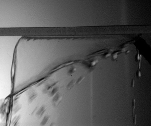
On hydrophilic surfaces (figure 6b), we find a significantly different topology. No rims are observed and the water spreads based on initial kinetic energy in all directions, as discussed in Kate et al. (Reference Kate, Das and Chakraborty2007), in the context of impingement on a top surface. For the range of parameters examined, water does not detach from the plate until it accumulates on the edges, once its advance is halted by frictional drag (Bhagat et al. Reference Bhagat, Jha, Linden and Wilson2018). Once enough water accumulates, gravity overcomes surface tension and a drop falls. The drops fall nominally vertically, which indicates that all momentum parallel to the plate was lost (see figure 8a). Droplets with a certain radius fall periodically from the edges, as was described previously for jet impacts on the underside of a hydrophilic flat plate by Jameson et al. (Reference Jameson, Jenkins, Button and Sader2010) and Brunet, Clanet & Limat (Reference Brunet, Clanet and Limat2004). An energy argument, similar to that described in (A1), but for spherical drops ((A6) and dashed line in figure 7), predicts the size of falling droplets to be around 8 mm, which is in fair agreement with observation in the present work (e.g. figure 8(a) shows falling droplets with diameters around 10 mm). Randomness in the location from which droplets detach may be caused by a Rayleigh–Plateau type instability, but further analysis would be needed to verify this.

Figure 6. Jet impingement with  $Q= 4.8\,{\rm l}\,{\rm min}^{-1}$, $d= 9.3\,{\rm mm}$ and $\alpha =45^{\circ }$ ( $\textit{Re} = 1.25 \times 10^{4}$, $\textit {We} = 231$). (a) Top view of patch on a hydrophobic surface (A2). Note the two thick perturbed (hence opaque) rims around a thin laminar (clear) region in the middle. (b) Top view of the patch on a hydrophilic surface (A1). The rims are absent, and water accumulates at the edges of the wetted spot from where drops detach (with radial accumulation location being time dependent). Note also the much larger wetted area on the hydrophilic surface. (c) Sketches of the approximated cross-section views at the lines indicated in (a,b); $\theta \approx \theta _{static}$ is the contact angle at the edge of the water patch.

Figure 7. Map of the experimental conditions and the critical rim diameter (see (A3)) above which the rim is expected to not be able to remain attached. Symbols indicate experimental observations: empty symbols indicate cases where the rims remained attached until they merged or water was stopped by viscosity and pooled on the edges; filled markers indicate that detachment was observed before rims merged. The dashed line (see (A6)) shows the critical diameter for droplets.

Figure 8. (a) Detachment from a hydrophilic surface (A1);  $Q= 2.46\,{\rm l}\,{\rm min}^{-1}$, $d= 6.1$ mm and $\alpha =35\,^{\circ }$ ( $\textit {Re} = 9.75 \times 10^{3}$, $\textit {We} = 212$). (b) Continuous rim/edge and film detachment on the superhydrophobic surface (A5); $Q= 4.62\,{\rm l}\,{\rm min}^{-1}$, $d= 9.3$ mm and $\alpha =45\,^{\circ }$ ( $\textit {Re} = 1.21 \times 10^{4}$, $\textit {We} = 214$).
3.1.1. Simplified criteria for water detachment
Seeking to better understand the different detachment behaviours observed on hydrophilic and hydrophobic surfaces, we derive in Appendix A a simplified model for a critical detachment rim radius of the water as a function of the surface contact angle. On hydrophobic surfaces, we could expect rims to detach from the underside of the plate if they had radius larger than that indicated in (A3). The critical rim diameter,  $2r_D(\theta )$, is plotted as a continuous line in figure 7. To the left of the line, the energy of the attached rim is lower than that of the detached rim, therefore we expect that it will preferably stay attached. To the right of the line, on the contrary, detachment is energetically favourable. In figure 7, each point represents the approximate rim diameter for all the pipe angles $\alpha$ and flow rate $Q$ for each surface and pipe size. Such a rim diameter was computed, as a first approximation, neglecting the flow rate through the thin laminar film between the rims. Detached (filled symbol) status was given to those flows where rims detached even before they merge (e.g. as seen in figure 8b), and attached (empty symbol) status indicates cases where rims detached only after merging (e.g. panel (d4) of figure 4), or a hydrophilic surface where the water accumulated at the edge of the patch and fell as droplets (figure 6b).
Equation (A3) predicted that on the mildly hydrophobic surface (A2), all but the largest jets are small enough to allow the water to remain attached, even if rims form. However, we see that rim separation (filled symbols in figure 7) required an  ${\approx }20\,\%$ larger equivalent rim diameter to detach than was predicted. Interestingly, if we do not neglect the flow rate in film between the rims and assume this to be ${\approx }30\,\%$ of $Q$, then the data points would be shifted to the left, matching the model's prediction.
Figure 7 shows superhydrophobic surfaces (A4 NaisolSHBC and A5 Cytonix800M) on the detached region of the graph, to the right of the borderline. In this case, where detachment is favoured from an energy balance viewpoint, we observe experimentally the rims or even the full film detach from the surface before the rims merge. For example, in figures 4(d4,d5) we see the rims detach, and in figure 8(b) even the full film detaches. For hydrophilic surfaces, where detachment is not energetically favourable, water detached in drops once forward momentum was lost and water accumulated in the path edges, as indicated by the droplets falling nearly straight down (figure 8a). (Similar droplet separations from surface considerations are provided e.g. in the numerical study of Manik, Dalal & Natarajan Reference Manik, Dalal and Natarajan2019).
3.2. Water patch width
Another key result of water spreading on surfaces is the maximum width. From conservation of mass, momentum and energy, we can attempt to predict the maximum width of the water patch as a function of the jet's vertical momentum, surface tension and contact angle. Appendix B discusses such a simplified model in detail. For a surface in Wenzel state, ignoring viscosity, we find that the water patch width is expected to scale with the contact-angle-modified Weber number of the perpendicular jet velocity component,  $We_{\theta z} = {\rho d u_z^{2}}/{\sigma (1- \cos \theta )}$ as
 \begin{equation} \frac{b_{max}}{d} = \frac{\rm \pi}{8 \cos{\alpha}}\,We_{\theta z} + \frac{\rm \pi}{\cos{\alpha}(1- \cos\theta)}. \end{equation}
The maximum water patch width is plotted in figure 9 against  $We_{\theta z}$. The model in (3.1) for smallest and highest $\alpha$ is represented by two lines.

Figure 9. Jet-width-normalized maximum water patch width versus contact-angle-modified vertical-velocity Weber number  $We_{\theta z}$. Lines show predictions of (3.1) for lowest and highest jet angle $\alpha$.
Data seem to collapse when plotted against the mentioned contact-angle Weber number (see figure 9), and furthermore, at low Weber numbers, the data also show a linear trend, albeit at a lesser slope than expected based on the simple analysis. However, the linear trend is lost as the jet speed increases, and viscous frictional losses could be expected to become non-negligible in the larger water patch. While (3.1) guided us to collapse the data with  $We_{\theta z}$, it is overly simplified especially in respect of ignoring friction.
A more comprehensive model was proposed by Wang et al. (Reference Wang, Faria, Stevens, Tan, Davidson and Wilson2013). Starting from the results of Wilson et al. (Reference Wilson, Le, Dao, Lai, Morison and Davidson2012), Wang et al. (Reference Wang, Faria, Stevens, Tan, Davidson and Wilson2013) construct a model for jet impingements on a vertical surface, accounting for oblique jet impact by incorporating the radial flow distribution model developed by Kate et al. (Reference Kate, Das and Chakraborty2007). While Wang et al. (Reference Wang, Faria, Stevens, Tan, Davidson and Wilson2013) are mainly concerned with jet impingement on a vertical surface, they also presented a model ignoring the effect of gravity, and such a model could be expected to more closely match the present data. The simplified version of this model yields the extent of the radial flow zone (corresponding to our patch width minus rim thickness) as a function of angular coordinate  $\psi$ and the impinging jet radius $r_0$:
 \begin{equation} r(\psi) = \left( \frac{9}{50} U^{3} \frac{\sin^{9}{\alpha}}{(1 + \cos{\alpha} \cos{\psi})^{6}}\,\frac{r_o^{6} \rho^{2}}{\mu \sigma(1-\cos{\theta})} \right)^{1/4}. \end{equation}
From this result, it is possible to obtain analytically the maximum width of the radial flow zone. Noting the width  $b = 2r(\psi ) \sin {\psi }$, we can obtain the maximum width by finding the maximum of the term $\sin ^{2}{\psi }/(1-\cos {\alpha } \cos {\psi })^{3}$ (Wang et al. Reference Wang, Faria, Stevens, Tan, Davidson and Wilson2013). Reorganizing terms, using $d = 2r_0$, and recognizing the modified Weber number ( $We_{\theta z}$) and Reynolds number ( $Re$), it is possible to express the maximum patch width as
 \begin{equation} \frac{b_{max}}{d} = 0.4606 \left( \frac{\sin^{7}{\alpha} \sin^{4}{\psi^{*}}}{(1 + \cos{\alpha} \cos{\psi^{*}})^{6}}\,We_{\theta z}\,Re \right)^{1/4}, \end{equation}
where  $\psi ^{*}$ corresponds to the azimuthal angle for maximum width obtained through the minimization of the $\sin ^{2}{\psi }/(1-\cos {\alpha } \cos ^{3}{\psi })$ term, such that
 \begin{equation} \cos{ \psi^{*}} = \frac{1 - \sqrt{1+3\cos^{2}{\alpha}}}{\cos{\alpha}}. \end{equation}
 The comparison of the predicted radial flow zone width to our data is presented in figure 10 and shows fair agreement with the experimental data. Although the trend is well captured, the tendency of the Wang et al. (Reference Wang, Faria, Stevens, Tan, Davidson and Wilson2013) model is to overestimate the radial flow zone width, even though our definition of the width also includes the rims. However, this overestimation of the patch width is not surprising as nothing in the models accounts for the tendency of gravity, particularly on superhydrophobic surfaces, to promote early dewetting. An extreme case of this is seen in figure 8(b), which shows a ‘skewed water bell’ where the film clearly separates from the plate before the radial spread was expected to end. A potential additional difference is that – contrary to the Wang et al. (Reference Wang, Faria, Stevens, Tan, Davidson and Wilson2013) assumption that all momentum of the flow along a streamline at all angles  $\psi$ is balanced by the surface tension at the edges of the radial flow zone – at maximum width (which does not occur at $\psi = 90^{\circ }$), the flow in the rims still carries momentum in the streamwise direction, and the boundary condition could be amended accordingly.

Figure 10. Comparison of measured patch width to width of radial spreading zone predicted by (3.3) based on model by Wang et al. (Reference Wang, Faria, Stevens, Tan, Davidson and Wilson2013).
3.3. Water patch length
The normalized water patch length is another quantity of interest. As seen in figure 11, it appears to scale approximately with the square root of the contact-angle-modified Weber number based on the horizontal,  $x$, jet velocity component:
 \begin{equation} We_{\theta x} = \frac{\rho d u_x^{2}}{\sigma(1-\cos\theta)}. \end{equation}
Figure 11. Jet-width-diameter normalized water patch length plotted against the square root of the contact-angle-modified horizontal-velocity Weber number,  $We_{\theta x}$.
We also note that a similar modified Weber number has been employed by e.g. Son & Kim (Reference Son and Kim2009) to characterize the spreading diameter of an inkjet droplet.
3.4. Water patch area
Given the trends of water patch width and length (the former scaling with the normal,  $z$, and the latter with the square root of the $x$-component with the contact-angle-modified Weber number), the water patch area was expected to potentially scale linearly with the square root of the product of the two contact-angle-modified Weber numbers. This assumption appears to be a fair approximation, as shown in figure 12.

Figure 12. Normalized water patch area plotted against the square root of the product of contact-angle-modified Weber numbers  $(We_{\theta i}=\rho u^{2}_{i}d/\sigma(1-\cos \theta))$.
3.5. Force on plate
Finally, the force on the plate was measured. Considering a control volume around the plate and encompassing the jet and water patch, the jet's momentum loss in the horizontal direction is equal to the measured force on the plate, if we assume air–water drag to be negligible:
 \begin{equation} F_{x} = \dot m u_x = \left(\rho U d^{2} \frac{\rm \pi}{4}\right) (U \cos{\alpha}), \end{equation}
where  $\alpha$ is the incident jet angle, nominally taken as the pipe angle, and $\dot m$ is the jet's mass flow rate.
In figure 13 the force measured by the load cell is plotted against the incoming jet's horizontal momentum, and (3.6) is plotted as a dashed line. Points on the dashed line hence correspond to cases where all of the jet's horizontal momentum is lost, and points below this line are cases where water departs the plate before losing all the momentum. We observe that most of the data for impingement of a hydrophilic surface (A1) lie on the line, thus indicating that all incoming horizontal momentum was lost due frictional drag. This is in good agreement with observations of water departing the glass as droplets with nominally no horizontal velocity, as seen in figure 14(b). Jet impingement on (super)hydrophobic surfaces populates below the line in figure 13, which indicates that water detaches from the low-energy surface before losing all its momentum. We see this in figure 14(a), where water departs the hydrophobic surface at nearly the same angle as it impacted.

Figure 13. Measured horizontal force on the plate versus horizontal momentum of the incoming jet; the dashed line represents (3.6), where these are equal and all horizontal momentum is lost due to viscous friction. Data below the line represent cases where only a fraction of the momentum was lost.

Figure 14. (a) ‘Rebound’ off the superhydrophobic plate (A5);  $Q= 2.58\,{\rm l}\,{\rm min}^{-1}$, $d= 6.1$ mm and $\alpha =25\,^{\circ }$. (b) Water departing vertically from a hydrophilic plate (A1); $Q= 1.98\,{\rm l}\,{\rm min}^{-1}$, $d= 6.3$ mm and $\alpha =25$ $^{\circ }$. The jet is at an oblique angle from the right.
From these data, we find the force on the plate to be dependent on the jet angle, jet velocity, surface properties and jet diameter. As we also have a measurement of the water patch area,  $A$, we can evaluate the frictional drag coefficient, $C_F = F_x / \frac {1}{2}\rho u_x^{2} A$. Figure 15 plots $C_F$ based on measured force and patch area against the Reynolds number $Re_L = \rho u_x L / \mu$ based on measured water patch length $L$ and horizontal velocity $u_x$. In this figure, we also show what $C_F$ would have been on a smooth surface simply assuming a ‘rectangular’ uniform patch with a Blasius laminar (dashed line) or Prandtl turbulent boundary layer (dash-dot line). For laminar flow, we also considered the nominally elliptical shape in the integration:
 \begin{equation} C_{f,LAM ellipse} = \frac{4}{{\rm \pi} b L}\int_0^{L} \int_{{-}b\sqrt{x/L(1-x/L)}}^{b\sqrt{x/L(1-x/L)}} \frac{0.664}{\sqrt{Re_x}} \,{{\rm d}y}\,{{\rm d} x} = \frac{1.13}{\sqrt{Re_L}}. \end{equation}
This result is shown in figure 15 as the solid line, which best matches the data on a hydrophilic (glass) surface.

Figure 15. Frictional drag coefficient  $C_F$ based on measured horizontal force $F_x$ and patch area $A$, versus $Re_L$. The dashed and dash-dot lines represent drag from turbulent and laminar approximations to the boundary layer friction coefficient, if we simplify the patch to be rectangular spanwise uniform. The solid line accounts for elliptical shape for a laminar boundary layer.
While the net force measured was smaller for superhydrophobic surfaces, a higher  $C_F$ was estimated based on patch area at given $Re_L$ (see figure 15). This suggests that in the present case, the force reduction is primarily a result of the reduction in the wetted area, and not due to drag reduction over the wetted area. That is, there is no clear sign of viscous shear stress reduction on the wetted patch due to the surface that may trap gas (as discussed in e.g. Gose et al. Reference Gose, Golovin, Boban, Mabry, Tuteja, Perlin and Ceccio2018). This may be due to roughness, or a lack of significant amounts of gas trapped on the surface perhaps due to the non-negligible jet impact velocity, similar to the case discussed in Zheng, Yu & Zhao (Reference Zheng, Yu and Zhao2005).
4. Results: effect of gravity
Previous studies on jets impacting vertical walls and top sides of surfaces provide interesting data for comparison in order to understand the effect of gravity. Results from four previous studies are used for comparison with current results: Kate et al. (Reference Kate, Das and Chakraborty2007) had a water jet impact the top of a surface and studied the hydraulic jump that resulted; Kibar et al. (Reference Kibar, Karabay, Yiğit, Ucar and Erbil2010) and Kibar & Yiğit (Reference Kibar2018) performed experimental work on water jet impingement on a vertical (super)hydrophobic surface; and Wang et al. (Reference Wang, Faria, Stevens, Tan, Davidson and Wilson2013) utilized experiment and theory to consider jet impingement on vertical hydrophilic surfaces. The parameter ranges that these investigators examined are compared to ours in tables 4 and 5. We proceed to a quantitative comparison of our data and the results from these previous studies. (And a more extensive qualitative comparison of different water patch topologies observed in the present work and in several other previous studies is provided in figure 18.)
Table 4. Range of surface parameters of the present and previous studies.

Table 5. Range of flow parameters of the present and previous studies.

4.1. Gravity's effect on the wetted area
Both Kate et al. (Reference Kate, Das and Chakraborty2007) and Wang et al. (Reference Wang, Faria, Stevens, Tan, Davidson and Wilson2013) theoretically, and later Kibar (Reference Kibar2018) by fitting experimental data, developed models to compute the radius of the water patch or hydraulic jump border depending on the azimuthal coordinate ( $r = r(\psi$), see figure 5). Kate et al. (Reference Kate, Das and Chakraborty2007) obtained the radial location of the hydraulic jump by applying the continuity and momentum equations to a radial slice of the flow. Assuming a quadratic velocity profile in the film, the following relation for the location of the hydraulic jump was obtained:
 \begin{equation} r(\alpha, \psi) = C \left( \frac{d^{2}}{8}\,\frac{\sin{\alpha}^{3}}{(1+\cos{\alpha} \cos{\psi})^{2}}\,U \right)^{5/8} \nu ^{{-}3/8} g^{{-}1/8}, \end{equation}
where  $C$ is a constant, $\nu$ is the water kinematic viscosity, $\psi$ is the azimuthal coordinate (see figure 5), $\alpha$ is the angle of the jet with the horizontal, and $g$ is the gravitational acceleration. (Note that the effect of the contact angle was not considered in (4.1).)
For jet impingement on a vertical hydrophilic surface, as discussed in § 3.2, Wang et al. (Reference Wang, Faria, Stevens, Tan, Davidson and Wilson2013) developed a model building on the results of Kate et al. (Reference Kate, Das and Chakraborty2007) and Wilson et al. (Reference Wilson, Le, Dao, Lai, Morison and Davidson2012), obtaining the water patch edge as the position at which the radial flow momentum is equal to the surface tension:
 \begin{equation} R(\psi) = \frac{3U\rho r_e^{2} \sin{\alpha}}{5\sigma (1 - \cos{\theta})}\,U_R(\psi), \end{equation}
where  $U_R(\psi )$ is the speed at the water patch edge $r=R(\psi )$, and $r_e$ is the radial position of the impinging jet (Kate et al. Reference Kate, Das and Chakraborty2007). The speed in the radial flow film can be obtained from a momentum balance as (Wang et al. Reference Wang, Faria, Stevens, Tan, Davidson and Wilson2013)
 \begin{equation} \frac{{\rm d}u}{{\rm d}r} ={-}10\,\frac{\nu}{U^{2} r_e^{4} \sin{\alpha}^{2}}\,r^{2} u^{2} - \frac{5g}{6}\,\frac{\cos{\psi}}{u}. \end{equation}
Neglecting gravity and assuming large water patches in comparison with the jet diameter ( $R\gg d$ and $U_R \ll U$), the above equation can be simplified to obtain (3.2). Since no gravity is included, (3.2) is of interest for impingement on horizontal surfaces.
Finally, Kibar (Reference Kibar2018), based on the experimental work in Kibar et al. (Reference Kibar, Karabay, Yiğit, Ucar and Erbil2010), found an empirical fit for the water patch that resulted from jet impingement on vertical (super)hydrophobic surfaces. The empirical fit that they found for the radial location of the water patch edge was
 \begin{equation} r(\psi) = \frac{d}{2} 0.2\,Re^{0.3}\,We^{0.4} [1 + \cos({\rm \pi} - \theta)]^{{-}0.5} \times \left[\frac{\sin^{2.2}\alpha}{1 + \cos{\alpha} \cos{\psi}} \right]^{1.34} \left[e^{\psi/{\rm \pi}}\right]^{0.65} \end{equation}
These theoretical and empirical equations (4.1), (4.2), (3.2) and (4.4), which the previous investigators found to match their data in a satisfactory manner, enable comparison of water patch topology depending on the plate's orientation i.e. effect of gravity (for a limited range of parameters, as the parameter ranges considered in present study only partially overlapped those previously considered, see tables 4 and 5).
A comparison of the water patch shape for a particular set of parameters is depicted in figure 16. All the shapes are similar, but enlarged by a factor that varies depending on the flow conditions, primarily differing in orientation of gravity. For most cases, the patch on the underside of the plate had an area between 1 and 5 times smaller than on vertical surfaces and the top side. This is not surprising given that in our case, water can detach once gravity overcomes surface tension.

Figure 16. Water patch shape comparison between current paper and equations found to fit results of: Kibar (Reference Kibar2018), see (4.4); Wang et al. (Reference Wang, Faria, Stevens, Tan, Davidson and Wilson2013), see (3.2) and (4.2); and Kate et al. (Reference Kate, Das and Chakraborty2007), see (4.1). Here,  $Q= 4.8\,{\rm l}\,{\rm min}^{-1}$, $d= 9.3$ mm, $\theta = 101^{\circ }$ and $\alpha =45^{\circ }$ ( $\textit {Re} = 1.25 \times 10^{4}$, $\textit {We} = 231$).
Figure 17 shows the average ratio of water patch length based on (4.1), (4.2), (3.2) and (4.4) with respect to that seen in the present study. Comparison with Kate et al. (Reference Kate, Das and Chakraborty2007) is particularly interesting. We observe that for a hydrophilic surface (in our case A1 Glass), the length ratio is approximately 1, which suggests that for the parameter range being considered and in the case of a hydrophilic surface, the dominant mechanisms are the same regardless of the orientation of gravity. That is, inertia and viscosity dominate the water patch size. On the top of a surface, a hydraulic jump results where momentum is mostly lost and jump conditions are met, whereas on the underside of a plate, the hydraulic jump is substituted by water accumulation at the corresponding location until gravity leads to droplet detachment, as discussed in § 3.1.1. However, when the surface impacted is hydrophobic, while still within parameter range of Kate et al. (Reference Kate, Das and Chakraborty2007), area ratio begins to increase. Surface tension still has the role of containing the water spread, but on the underside of a plate, gravity facilitates dewetting when the two rims merge (e.g. panels (b1) and (b2) of figure 4), or even before (e.g. figure 8b). The key difference is that with the present orientation of gravity, the impingement does not need to result in a hydraulic jump, but rather fluid can dewet the surface prior to a hydraulic jump.

Figure 17. Mean length ratio for Kibar (Reference Kibar2018), Wang et al. (Reference Wang, Faria, Stevens, Tan, Davidson and Wilson2013) (g for gravity included, (4.2), and ng for no gravity, (3.2)) and Kate et al. (Reference Kate, Das and Chakraborty2007) with respect to this paper. Each bar value is the average of the ratio of all the tests done of such surface (51 for A1 Glass, 68 for A2 NeverWet, 35 for A4 NaisolSHBC, and 64 for A5 Cytonix800M). The error bars represent one standard deviation.
Comparison to a water patch on a vertically orientated surface of Wang et al. (Reference Wang, Faria, Stevens, Tan, Davidson and Wilson2013) (with gravity, (4.2)) and Kibar (Reference Kibar2018) shows that the water patch length is 2–5 times that found in the present study. However, when gravity is omitted from the model, Wang et al. (Reference Wang, Faria, Stevens, Tan, Davidson and Wilson2013) is closer to this paper's results. Note also that the width that Wang et al. (Reference Wang, Faria, Stevens, Tan, Davidson and Wilson2013) predict is that of the radial flow zone alone, and our definition of the water patch width includes this zone and the rims. Hence a ratio slightly below unity would indicate that the model prediction matches the present data. In these previous studies, surface tension had a role along with viscosity and inertia, and gravity aided the spread of the fluid but did not promote dewetting. This differs from the case in the present study, where gravity aids the dewetting from the underside of the surface, resulting in smaller water patch areas.
Furthermore, to check if changing the orientation of gravity would have a similar effect on topology resulting from jet impingement on our specific surfaces, a quick and rough qualitative experiment was conducted by affixing a pipe at an angle to one of our plates (A4). When manually varying the angle of the entire set-up, an increase in wetted patch area was observed, and this was qualitatively in agreement with Wang et al. (Reference Wang, Faria, Stevens, Tan, Davidson and Wilson2013); Kibar (Reference Kibar2018). Hence for this type of experiment and parameter range, a relatively low Froude number and orientation of gravity appear to have a major role in determining the water patch area.
4.2. Gravity's effect on force imparted on plate
In Kibar et al. (Reference Kibar, Karabay, Yiğit, Ucar and Erbil2010), which spanned  $\textit {Re} = 500\text {--}8000$, $\textit {We} = 5\text {--}650$, $\alpha = 15\text {--}45^{\circ }$, and examined surfaces with $\theta = 102^{\circ }, 112^{\circ }, 123^{\circ }, 145^{\circ }, 167^{\circ }$, the force ratio with respect to the momentum of jet imparted on the plate was found to have fair agreement with an empirical fit given by
 \begin{equation} \frac{F_x}{M_{jet,x}} = 0.911\,Re^{0.481}\,We^{{-}0.524} (1+\cos(180-\theta))^{{-}7.188} \sin(\alpha)^{0.529} \left(\frac{4A}{{\rm \pi} d^{2}}\right)^{0.690}, \end{equation}
where  $M_{jet,x} = \rho Q U\cos (\alpha )$. When (4.5) is applied to our full range of parameters, non-physical results exist that exceed the force–momentum ratio of unity. However, if only cases within the range of data of (Kibar et al. Reference Kibar, Karabay, Yiğit, Ucar and Erbil2010) are considered, then the effect of gravity being parallel to the plate (where the plate is in a vertical position as in Kibar et al. Reference Kibar, Karabay, Yiğit, Ucar and Erbil2010) significantly increases the force on the plate (around an order of magnitude for a glass surface, by a factor of 3–5 times in the case of (super)hydrophobic surfaces). This is presumably due to the significantly increased contact area and allowing for increased effect from frictional drag.
However, as only a small number of cases in the present study overlap with Reynolds and Weber numbers considered in Kibar et al. (Reference Kibar, Karabay, Yiğit, Ucar and Erbil2010), whose empirical correlation cannot be extrapolated beyond the original parameter range, further study would be needed to quantify the effect of orientation on jet momentum loss (i.e. force on the plate).
4.3. Gravity's effect on the topology
While qualitatively similar topology to figures 4 and 6 was found for jet impingement on vertical and horizontal (super)hydrophobic surfaces in Kibar (Reference Kibar2018), Kibar et al. (Reference Kibar, Karabay, Yiğit, Ucar and Erbil2010) and Kaps et al. (Reference Kaps, Adelung, Scharnberg, Faupel, Milenkovic and Hassel2014), in general, multiple topologies can be identified for jet impingement on surfaces depending on the orientation of gravity. Figure 18 shows the various topologies reported for different orientations of gravity and contact angle, as well as those seen in the present study (panel (e) right, and (f) left and right).

Figure 18. Different water patch topologies and flow patterns reported depending on plate orientation and contact angle. (a) Hydraulic jumps as seen in Kate et al. (Reference Kate, Das and Chakraborty2007). (b) Braiding as seen in Mertens, Putkaradze & Vorobieff (Reference Mertens, Putkaradze and Vorobieff2005), and reflections for microjets as in Celestini et al. (Reference Celestini, Kofman, Noblin and Pellegrin2010). (c) Vertical rivulet flow (Wilson et al. Reference Wilson, Le, Dao, Lai, Morison and Davidson2012), gravity and dry patch flow (Wang et al. Reference Wang, Faria, Stevens, Tan, Davidson and Wilson2013). (d) Braiding and reflection of jet as per Kibar et al. (Reference Kibar, Karabay, Yiğit, Ucar and Erbil2010). (e) Underside waterbells for limited range of flow conditions of Button et al. (Reference Button, Davidson, Jameson and Sader2010), and droplet detachment as seen both in Button et al. (Reference Button, Davidson, Jameson and Sader2010) and in the present study on surface A1. (f) Reflection before rims join, forming a skewed water bell, and reflection when rims merge, as seen in the present study on surfaces A2, A4 and A5.
With respect to a jet impinging on the top side of a hydrophilic horizontal plate, several topologies of hydraulic jumps are explained and modelled in (Kate et al. Reference Kate, Das and Chakraborty2007). Braiding appears when the surface starts to transition towards the hydrophobic region (Celestini et al. Reference Celestini, Kofman, Noblin and Pellegrin2010) or when the plate has some inclination with respect to gravity (Mertens et al. Reference Mertens, Putkaradze and Vorobieff2005). Finally, reflections were seen when very high surface hydrophobicity and small jets were used (Celestini et al. Reference Celestini, Kofman, Noblin and Pellegrin2010).
If the plate is vertical, then rims form on the edges of the water patch, resulting in rivulet flow at low flow rates (Wilson et al. Reference Wilson, Le, Dao, Lai, Morison and Davidson2012), and when the jet flow rate increased, ‘gravity’ or ‘dry patch’ patterns (figure 18c) have been reported (Wang et al. Reference Wang, Faria, Stevens, Tan, Davidson and Wilson2013). Higher angles of jet impingement,  $\alpha$, or jet momentum tend to lead to what authors called ‘gravity’ flow, while increasing the contact angle (albeit within the hydrophilic region) increased the tendency for rivulet and dry patches. That is, as in the present study, increased hydrophobicity reduced the surface-water contact area. If the vertical walls’ contact angle is increased above $90^{\circ }$ into the hydrophobic and superhydrophobic ranges, then braiding was reported for lower contact angles and jet flow rate, while higher values of these parameters led to transition towards reflection, and even splashing (i.e. disorganized reflection).
Finally, if the jet impinges on the underside of a horizontal hydrophilic surface, as in the present study (figure 8a), the result was droplet detachment from the edges. Interestingly, for a laminar jet impinging normal to a surface, and for a special combination of parameters, a water bell topology may also result as in Button et al. (Reference Button, Davidson, Jameson and Sader2010). In the present study, if surface hydrophobicity is increased, then reflection can be observed (similar to that seen in the case of vertical surfaces), although the water patch area is greatly reduced. And a skewed-water-bell-type detachment (figure 8b) could be observed in some particular cases.
Comparing to previous hydrophobic surface experiments where the orientation of gravity was different, the jet impinging on the plate's underside differs notably: e.g. the rims do not reappear after merging, and a second patch never forms for the parameter range studied. For all conditions examined, once the rims merge, water detaches from the plate in a jet-like topology. This is substantially different from observations of Kibar et al. (Reference Kibar, Karabay, Yiğit, Ucar and Erbil2010), who studied a jet with parameter range overlapping ours and reported oscillation between open and closed rims, i.e. ‘braiding’. This braiding could be considered to be the two-dimensional (due to the physical surface) equivalent to fluid chains studied in context of two liquid jets impinging in air (e.g. Bush & Hasha Reference Bush and Hasha2004), and qualitative similarity to flows of the present study can be noted in the rim and film topology. However, differences arise due to the effect of gravity, because of the present study's lower Froude numbers and the presence of a solid surface.
5. Results: effect of roughness
We also conducted exploratory experiments on the effect of surface roughness on the flow topology. Surfaces B1 (smooth) and B2 (rough), described in table 1, have similar contact angles, but B2 is hydraulically rough. For water patch area, shown in figure 19, we can see a trend: for low jet momentum, the wetted area on surfaces is similar. However, beyond a ‘critical’  $\sqrt {We_{\theta z}We_{\theta x}} \approx 60$, the smooth surface's wetted area is more than double the size of that on the rough surfaces.

Figure 19. Water patch area on rough (B2) and smooth (B1) surfaces normalized by jet cross-section plotted against the square of the product of the contact-angle-modified Weber numbers.
Considering the low Weber number region where the viscous sublayer would be thicker, it could be that effectively both surfaces present to the flow as hydraulically smooth in this range. As the viscous sublayer becomes thinner at higher velocities (higher  $We$), the surface of the B2 plate becomes hydraulically rough, and lower water patch areas occur due to higher momentum loss as a result of increased skin friction.
Jet impingements at three different flow rates are shown in figure 20. The images in figure 20(a) correspond to the smooth surface, while those in figure 20(b) show the rough plate. We clearly see what the data in figure 19 indicated: the water patch grows faster with increased jet momentum on the smooth surface. However, as we examined only one rough plate, and the manual surface production may have resulted in inhomogeneities, one should view these preliminary results with caution. To gain further insight into roughness effects, a followup study is planned.

Figure 20. Top view of the water patch on (a) smooth surface (B1), and (b) rough surface (B2). From top to bottom, the flow rates are 7.71, 5.78 and  $3.86\,{\rm l}\,{\rm min}^{-1}$ ( $\textit {Re} = 2.01 \times 10^{4}$, $\textit {We} = 596$; $\textit {Re} = 1.51 \times 10^{4}$, $\textit {We} = 335$; $\textit {Re} = 1.01 \times 10^{4}$, $\textit {We} = 149$). The pipe diameter ( $d$) was 9.3 mm, and the incidence angle ( $\alpha$) was $25^{\circ }$.
6. Conclusions
The flow topology and horizontal force imparted by a water jet impinging on the underside of a flat plate were studied over a range of parameters. The surfaces’ hydrophobicity was found to be the key parameter, and momentum loss and wetted area were found to increase with a lower surface contact angle. Regarding topology, two distinct flow behaviours were observed.
(i) For hydrophilic surfaces, both viscosity and gravity versus surface tension play dominant roles: first viscosity slows down the water until it is accumulated at the boundaries of the patch, then gravity causes droplets to fall once they grow too large (i.e. when energy is minimized by detachment).
(ii) Jet impingement on a (super)hydrophobic surface formed an ellipse shape delimited by two rims that carry the majority of the flow and enclose a laminar thin film. The interchange between kinetic energy and surface tension resembles that of a harmonic oscillator, with surface tension as the spring. The rims open up until a maximum width is reached where all lateral kinetic energy is transformed into surface energy. This is then transformed back to lateral inward kinetic energy during the second half of the water patch.
For a narrow range of parameters, reflection could occur before the rims merge, while the film remains connected to the rims and separates from the surface downstream (e.g. figure 8b). This could be thought of as a type of skewed water bell that appears to be rather unique. A simplified model for rim detachment was found to describe the observations fairly well.
Water patch width dependency on various parameters was studied and inspired the scaling with modified Weber number  $We_{\theta z}$ that collapsed data. A simple model without friction aided understanding, but overpredicted patch width. A model based on Wang et al. (Reference Wang, Faria, Stevens, Tan, Davidson and Wilson2013), which accounted for friction, provided a somewhat more satisfactory scaling, albeit it still overpredicted the width. However, this could have been expected as nothing in any of the models considered in the literature or present work accounts for the tendency of gravity to promote dewetting. This was seen particularly on the superhydrophobic surfaces, where, in an extreme case (see figure 8b), a ‘skewed water bell’ – where the film separates from the surface before the radial spread was predicted to end – was observed. An additional cause for the Wang et al. (Reference Wang, Faria, Stevens, Tan, Davidson and Wilson2013) model's overprediction is that contrary to the momentum of the flow along a streamline at all angles $\psi$ being balanced by the surface tension at the edges of the radial flow zone, as assumed in Wang et al. (Reference Wang, Faria, Stevens, Tan, Davidson and Wilson2013), at maximum width, $\psi$ is not $90^{\circ }$ and the flow in the rims carries momentum in the streamwise direction. Hence in a future study modified boundary conditions should be explored.
The measured horizontal force, equivalent to the momentum loss of the jet, was shown to be sensitive to surface properties. While on a hydrophilic surface nominally all horizontal momentum was lost before detachment, on a hydrophobic surface the jet often detached with a significant fraction of its horizontal momentum remaining. This, along with a smaller water patch area, may also in part explain observations made in context of air layer drag reduction on hydrophilic and hydrophobic surfaces Peifer et al. (Reference Peifer, Callahan-Dudley and Mäkiharju2020) and Callahan-Dudley et al. (Reference Callahan-Dudley, Tecson, Martinez de la Cruz and Mäkiharju2020). These data suggest that water encountering a hydrophobic surface would be returned to the bulk flow not only sooner and after having wetted a smaller area, but also with more of its original streamwise momentum left. The latter could lessen the probability for generating another rewetting event, as the returning fluid mixes with bulk flow with nearly uniform velocity, instead of returning having lost all its momentum and hence possibly promoting overturning.
As opposed to Bush & Hasha (Reference Bush and Hasha2004), where gravity was justifiably negligible, and by the nature of the two jets colliding there was no surface friction, the present work considered a significantly lower Froude number region. Hence it was not surprising that orientation of gravity was found to be non-negligible. Interestingly, in the present study, in some parameter ranges, the droplet ejection from the rims seen in high-speed recordings was reminiscent of ‘fishbone’ formation discussed in Bush & Hasha (Reference Bush and Hasha2004). Given  $Re$,
$Re$,  $We$ and $Oh(\sqrt{(We)/Re})$ the range may be also due to a Rayleigh–Plateau type instability. However, the data collected in the present study do not lend themselves to an in-depth analysis of such instabilities. Specifically, we see that compared to the flows at similar parameter ranges of Kate et al. (Reference Kate, Das and Chakraborty2007), Wang et al. (Reference Wang, Faria, Stevens, Tan, Davidson and Wilson2013) and Kibar (Reference Kibar2018), a different orientation of gravity modified the wetted patch area, force imparted and overall topology.
Data from exploratory experiments on hydraulically rough surfaces also suggest that surface roughness can significantly affect the resulting water patch area. Water spread on smooth surfaces surpassed that on rough coatings as the Weber number was increased. Further study is needed to enable a clearer explanation of the mechanisms by which roughness in conjunction with hydrophobicity effects the topology.
Finally, we may also note that a scaling of the water patch area was found with the contact-angle-modified Weber number,  $We_{\theta }$, which successfully predicted the fraction of wetted surface in experiments of air layer drag reduction on hydrophilic and hydrophobic surfaces (Callahan-Dudley et al. Reference Callahan-Dudley, Tecson, Martinez de la Cruz and Mäkiharju2020). Despite the numerous approximations, the effect of contact angle on air layer integrity was matched qualitatively. Hence the present results begin to offer insight to a scaling that may explain data of Peifer et al. (Reference Peifer, Callahan-Dudley and Mäkiharju2020) and Callahan-Dudley et al. (Reference Callahan-Dudley, Tecson, Martinez de la Cruz and Mäkiharju2020). However, further studies to enable more general quantitative prediction and consideration of roughness are needed, and such research is ongoing.
Acknowledgements
Thanks to the Justus & Louise van Effe Grant (TU Delft) for making life at Berkeley possible financially; to PhD students at UC Berkeley, K. Kadala for aiding with the contact angle measurements, and D. Grieb for helping to set up the flow loop; to C.M. Reynaud for working with R.M. during the last few months of his studies, and continuing to collect and analyse additional data during his summer visit to Berkeley; and to undergraduate students T. Streichenberger and K. Chrismanto, who helped to characterize the plates.
Funding
This research received no specific grant from any funding agency, commercial or not-for-profit sectors.
Declaration of interests
The authors report no conflict of interest.
Appendix A. Water detachment criteria
We consider rim detachment criteria based on an energy balance analysis with the simplifications stated below. We consider for such an analysis the two possible states of a rim at any given point of the ellipse edge, depending on the rim water volume and the surface properties.
(i) The rim remains attached to the surface. As sketched in figure 6(c), we assume that the rim forms a partial cylinder with a contact angle nominally equal to the static surface contact angle $\theta$ (defined in radians for definitions of table 6), and a constant volume $V$ per unit length, $\Delta L$, which determines the attached partial cylinder's radius, $r_A$.
(ii) The rim is fully detached from the surface, but is still tangent to the surface. With a radius
$r_D$, it is taken to have a circular cross-section (figure 21).


Figure 21. Rims cross-section sketch used for energy balance model for attached (a) versus detached (b) rims. Here,  $\theta$, $r_A$, $r_D$ and $c$ represent the contact angle, attached drop radius, detached drop radius and centroid distance to the surface, respectively. The $A$ terms represent different areas per unit length according to table 6.
Table 6. Areas and volumes per unit length, and centroids, of the attached and detached cylinder cross-sections as functions of contact angle,  $\theta$, and their radii, $r_A$ and $r_D$. The two radii are related by mass conservation as $V^{A} = V^{D}$, $r_A^{2}={2 {\rm \pi}r_D^{2} }/({2\theta - \sin 2\theta })$.

The volume per unit length,  $V$, contact area between solid and liquid, $A_{SL}$, area between liquid and gas when detached $A_{LG}^{D}$, and attached $A_{LG}^{A}$, new area created between gas and solid when water is detached, $A_{SG}^{D}$, and centroid, $c$, can all be computed as functions of the contact angle, $\theta$, attached cylinder radius, $r_A$, and detached radius, $r_D$. Table 6 summarizes these values, and some are depicted in figure 21.
The question that we are trying to answer is: what is the energy associated with each of these two states, and for which surface properties and rim size is one more favourable than the other? (That is, where is the limit where, energetically, it is more efficient to stay attached or detach from the surface?)
In other words, we seek to obtain the critical rim volume at which the energies of the attached and detached states are equal. Volume per unit length any larger than this critical value would lead to rim detachment. Establishing an energy balance between the two cases, assuming insignificant kinetic energy difference between the attached and detached rims states, and taking into account surface tension and gravitational potential energies, we can write
 \begin{equation} A^{A}_{LG} \sigma_{LG} + A^{A}_{SL} \sigma_{SL} - \rho V^{A} g c^{A} = A^{D}_{LG} \sigma_{LG} + A^{D}_{SG} \sigma_{SG} - \rho V^{D} g c^{D}, \end{equation}
where the superscripts  $A$ and $D$ indicate the attached and detached values from table 6, respectively; $g$ is the gravitational acceleration; $\rho$ is the water density, and $\sigma$ is the surface tension between the mediums indicated with the subscripts $S,L,G$ (solid, liquid, gas). Note the negative sign in front of the potential energy terms, as the zero potential energy line is taken at the plate height and positive upwards.
Using Young's equation to relate the surface tension forces at the triple point and the contact angle ( $\sigma _{SG} - \sigma _{SL} = \sigma _{LG}\cos \theta$), and realizing that the detached solid–gas area is equal to the attached liquid–solid area ( $A^{D}_{SG} = A^{A}_{SL}$), we can eliminate the unknown solid–gas and liquid–solid surface tension, replacing it by the contact angle ( $\theta$):
 \begin{equation} \sigma_{LG} ( A^{A}_{LG} -A^{D}_{LG}-A^{A}_{SL} \cos\theta)-\rho g (V^{A} c^{A}-V^{D} c^{D}) = 0, \end{equation}
where  $\sigma _{LG}$, or just $\sigma$ as defined earlier, is the air–water surface tension.
Introducing the values in table 6 into (A2) and relating the detached and attached cylinder radii by the cylinder cross-section constant volume per unit length, we find
 \begin{equation} r_D|_{cylinder} = f(\theta) = \sqrt{2\,\frac{ \sigma}{\rho g}\,\frac{A_c (\theta)}{ B_c(\theta)}}, \end{equation}
where
 \begin{gather} A_c(\theta) = {\rm \pi}+ \left(\frac{2{\rm \pi}}{2\theta-\sin(2\theta)}\right)^{1/2} (\sin\theta \cos\theta-\theta), \end{gather}
 \begin{gather}B_c(\theta) = {\rm \pi}- \left(\frac{2{\rm \pi}^{3}}{2\theta-\sin(2\theta)}\right)^{1/2} \left(\frac{4 \sin^{3}\theta}{3(2\theta-\sin(2\theta))} - \cos\theta\right). \end{gather}
To consider when droplets might separate from the rims formed on the hydrophobic surfaces or from the accumulation on the edges of the patch on the hydrophilic surface A1, we repeat a similar energy analysis for droplets as discussed for cylinders above. This analysis will result in (A6) given below (and shown as a dashed line in figure 7):
 \begin{equation} r_D|_{droplet} = f(\theta) = \sqrt{\frac{\sigma\,A_d (\theta)}{\rho g\,B_d(\theta)}}, \end{equation}
where
 \begin{gather} A_d(\theta) = {\rm \pi}\left[ (2-2 \cos\theta)((1- \cos\theta)(2+ \cos\theta))^{2/3} - \sin^{2}\theta \cos\theta \right], \end{gather}
 \begin{gather}B_d(\theta) = \frac{\rm \pi}{3} \left[ (1- \cos\theta)^{2}(2+ \cos\theta) \left( \frac{3+3 \cos\theta}{2+ \cos\theta} - 4 \cos\theta -(1\!-\! \cos\theta)^{2}(2\!+\! \cos\theta) \right) \right]. \end{gather}
This predicts the size of droplets that should detach (e.g. from the hydrophilic surface A1 as water accumulates on the edges and form drops too heavy for surface tension to keep them attached). The prediction is in fair agreement with observation. Figure 8(a) shows detached drops from the A1 surface to be  $\approx$6–10 mm in diameter, whereas (A6) predicted $\approx$8 mm to be the critical droplet diameter for detachment for surface A1.
Appendix B. Water patch width prediction
A simplified model is introduced in an attempt to better understand the dependence of the water patch maximum width on hydrophobic surfaces described in § 3.1. The approach chosen is inspired by Kaps et al. (Reference Kaps, Adelung, Scharnberg, Faupel, Milenkovic and Hassel2014), who asserted previously that the jet velocity  $x$-component plays a minor role in the patch maximum width, and similarly, as a first approximation, we consider the jet's $x$-momentum to remain unchanged in the control volume. Mass, momentum and energy conservation are applied in the control volume shown in figure 22. The control volume begins at the jet exit from the pipe, terminating at the broadest point of the water patch on the surface. To simplify the analysis we assume the following.
(a) Steady state.
(b) Constant density, temperature and ambient pressure.
(c) Water loss from the rims before the location of maximum width is taken to be insignificant (i.e. water enters and exits the control volume solely via the jet and patch cross-section surfaces). Note that for the parameter range considered, this assumption was justified by observations as the modest momentum of film flow in the negative
$x$-direction was less significant than surface tension in the $x<0$ region. However, one should note that were the parameters to be expanded beyond the range considered, especially if the angle were to approach 90$^{\circ }$, water loss in the negative $x$-direction could become significant.(d) The cross-section at the widest point of the patch is approximated to be rectangular and to have a uniform velocity. (Note that figure 6(c) shows a more realistic cross-section that one should consider in a more detailed analysis.)
(e) Incoming jet velocity is nominally uniform.
( f) Frictional drag is neglected in the water–plate and water–air interfaces.


With the included approximations, the conservation laws for the control volume can be written as follows.

Figure 22. Sketch of control volume (red) used for derivation of a simplified model for the water patch width. Side view shown in panel (b), and cross-section at indicated plane in (a). Note that figure 6(c) shows a more realistic cross-section, and the rectangular approximation is adopted only for the present analysis. With this first approximation, the water patch shape is considered to be a  $b \times t$ rectangle, while in actuality the cross-section consists of rims connected by a thinner film.
Conservation of mass:
With the above approximations and for convenience taking  $z$ as positive along the gravity vector, we have
 \begin{equation} \rho b_{max} \int_{0}^{t} u_x(y) \,{\rm d}z = \rho 2 {\rm \pi}\int_{0}^{d/2} u_{axial}(r)\,r \,{\rm d}r. \end{equation}
Assuming uniform velocity at both inlet and outlet, and as by definition the measured mass flow and average jet velocity  $U$ are related by $U = 4\dot m / \rho {\rm \pi}d^{2}$ and density is constant, we have
 \begin{equation} U_{out} b_{max} t = {\rm \pi}\frac{d^{2}}{4} U. \end{equation}
Conservation of linear momentum in x-direction:
This is given for the control volume by
 \begin{equation} D_{on plate} = \dot m_{out} U_{out} - \dot m_{in} \cos(\alpha)\,U, \end{equation}
which, if drag were negligible and given that  $\dot m_{in} = \dot m_{out}$, simplifies to
 \begin{equation} U_{out} = U \cos{\alpha}. \end{equation}
Conservation of energy:
Assuming constant temperature and pressure, we consider only the surface, kinetic and potential energies, with subscripts  $s$,
$s$,  $k$ and $p$, respectively. We can hence write
 \begin{equation} \dot E_{s,in} + \dot E_{k,in} + \dot E_{p,in} = \dot E_{s,out} + \dot E_{k,out} + \dot E_{p,out}. \end{equation}
Note as well that the liquid–air interface area ( $A_{LG,out}$) is computed neglecting the extra interface surface from the rims’ curvature and film thickness, which can be estimated to cause an approximately 2 % error. Hence, considering the simplified rectangular cross-section, we obtain
 \begin{align} &{\rm \pi} d U \sigma_{LG} + \tfrac{1}{2} \dot m_{in} U^{2} + z_{pipe} g \dot m_{in} \nonumber\\ &\quad = U_{out} [ \phi \sigma_{SL} b_{max} + [(1-\phi)b_{max} +(2t + b_{max}) ]\sigma_{LG} - \phi \sigma_{SG} b_{max}]\nonumber\\ &\qquad + \tfrac{1}{2} \dot m_{out} U_{out}^{2} \nonumber\\ &\qquad + \tfrac{1}{2} ({-}1) t g \dot m_{out}, \end{align}
where  $\sigma _{LG}$, $\sigma _{SL}$, $\sigma _{SG}$ are the surface tensions of the liquid–air, liquid–solid and solid–air interfaces, and $\phi$ is the wetted fraction of the surface. Finally, note that $z_{pipe}$ is negative.
Using Young's equation to incorporate the contact angle instead of the solid–gas and solid–liquid surface tensions, assuming  ${t}/{b_{max}} \ll 1$ and reorganizing terms, gives
 \begin{align} &{\rm \pi} d \sigma_{LG} + \tfrac{1}{2} \rho {\rm \pi}\frac{d^{2}}{4} U^{2} + \left(z_{pipe} + \tfrac{1}{2} t\right) g \rho {\rm \pi}\frac{d^{2}}{4} \nonumber\\ &\quad= \cos{(\alpha)}\,b_{max} \sigma_{LG} [ - \phi \cos{\theta} + 2 - \phi ] \nonumber\\ &\qquad + \tfrac{1}{2} \rho {\rm \pi}\frac{d^{2}}{4} [\cos^{2}({\alpha}) U^{2}]. \end{align}
 Finally, solving for  $b_{max}$ gives
 \begin{align} \frac{b_{max}}{d} &= \frac{{\rm \pi} \rho d u_z^{2} }{8 \sigma_{LG} [2 - \phi (1 + \cos{\theta} ) ]\cos{\alpha}}\nonumber\\ &\quad + \frac{\rm \pi}{[2 - \phi (1 + \cos{\theta} ) ]\cos{\alpha}} + \frac{d \left(z_{pipe} + \frac{1}{2} t\right) g \rho {\rm \pi}}{4 \sigma_{LG} [2 - \phi (1 + \cos{\theta} ) ]\cos{\alpha}}. \end{align}
 We note that for the (super)hydrophobic cases (A3, A4, A5), the wet fraction value is unknown, as a Cassie state may exist. However, as detailed in § 3.5, for the jet velocities used, the water in contact with the surface might be in a Wenzel state ( $\phi =1$). If the wet fraction ( $\phi$) is considered to be 1, meaning that all the surface in between the water and plate is wetted, and recognizing the term ${\rho d u_z^{2}}/{\sigma _{GL}(1- \cos \theta )}$ as the contact-angle-modified Weber number of the perpendicular jet velocity component, $We_{\theta z}$, then we find
 \begin{equation} \frac{b_{max}}{d}\,\frac{\cos{\alpha}}{\rm \pi} = \frac{We_{\theta z}}{8} + \frac{1}{[1 - \cos{\theta}]} + \frac{d \left(z_{pipe} + \frac{1}{2} t\right) g \rho}{4 \sigma_{LG}[1 - \cos{\theta}]}. \end{equation}
Here,
 \begin{equation} \frac{d \left(z_{pipe} + \frac{1}{2} t\right) g \rho}{ \sigma_{LG}[1 - \cos{\theta}]} \end{equation}
could be termed as a modified Bond (Eötvos) number  $Bo_{dz}$ as it relates the relative importance of the gravitational forces (elevation change) to surface tension:
 \begin{equation} \frac{b_{max}}{d}\,\frac{\cos{\alpha}}{\rm \pi} = \frac{We_{\theta z}}{8} + \frac{1}{[1 - \cos{\theta}]} + \frac{Bo_{dz}}{4}. \end{equation}
Examining the magnitude of the modified Bond term compared to others, we find it to be always below  $20\,\%$, and below $5\,\%$ for most cases. Hence we could simplify this to
 \begin{equation} \frac{b_{max}}{d} = \frac{\rm \pi}{8 \cos{\alpha}}\,We_{\theta z} + \frac{\rm \pi}{\cos{\alpha}[1- \cos\theta]}. \end{equation}
Appendix C. Dimensional analysis
Table 2 summarizes the dimensional independent variables in this study, and ranges of their values, namely pipe diameter  $d$, nominal jet velocity $U$ (taken to be equal to the average velocity in the pipe), jet angle $\alpha$ (nominally equal to pipe angle), surface contact angle $\theta$, surface roughness $R_a$, water–air surface tension $\sigma$, water dynamic viscosity $\mu$, water density $\rho$, and gravity acceleration $g$. Flow rate would be redundant, as it can be constructed from the jet velocity and pipe diameter. These nine variables determine the output from the system, among which are the water patch area $A$, length $L$, maximum width $b_{max}$, and horizontal force $F_x$. Applying Buckingham's ${\rm \pi}$ theorem, four dependent groups containing the output variables above can be considered to be dependent on only six non-dimensional groups, all summarized in table 7. Additional dimensionless numbers, all derived from the ones included in table 7, and used throughout the present study, are as follows.
(i) Contact angle-modified Weber number,
$We_\theta$. This appears when analysing the energy balance of the spreading film taking into account surface tension (B12). It is therefore an expansion of the classical Weber number when surface tension effects become important, and is derived from the Weber number and the contact angle. Depending on the wetting model, different versions of this derived non-dimensional number may be relevant.(ii) Froude number,
$Fr$. This relates the flow inertia to the gravity, and is particularly interesting due to the connection between the present study and naval applications. It is derived from the Weber and Bond numbers as $Fr = \sqrt {{We}/{Bo}}$.(iii) Non-dimensional roughness,
$k^{+}$. The relative roughness, $\epsilon$, gives a physical ratio between the characteristic dimension, taken as jet diameter in the present study, and physical surface roughness. However, from a general fluid dynamics point of view, it is the non-dimensional roughness, $k^{+}$, that determines if the height of the surface peaks and valleys is sufficient that they protrude through the viscous sublayer and have an influence on the flow over the surface. This is constructed as $k^{+} = {\rho u_\tau k_s}/{\mu }$, where $k_s \approx 5.86\,R_a$ (Adams et al. Reference Adams, Grant and Watson2012), and $u_\tau$ is the frictional velocity based on measured force and water patch size.


Table 7. Set of four dependent and six independent groups resulting from the dimensional analysis. Alternative groups can be derived from these, and of particular interest in the present study is the contact-angle-modified Weber number.

Appendix D. Raw data
Table 8 shows the data in raw format to facilitate further comparison to theory and other experiments. Uncertainties based on instrumentation or standard deviation of a number of measurements were below 0.1 mm for pipe diameter  $d$,
$d$,  $1.5^{\circ }$ for pipe angle $\alpha$, $0.08\,{\rm l}\,{\rm min}^{-1}$ for flow rate $Q$,
$Q$,  $8^{\circ }$ for the contact angle $\theta$, 4 mm for the length $L$ and maximum width $b_{max}$ of the ellipse, and $0.003$ N for the horizontal force $F_x$.
Table 8. Raw data for the superhydrohphobic ‘A’ surfaces.


 Open access