


Introduction
The Groningen field was discovered in 1959 and gas production started in 1963. Globally, the field is one of the top ten largest gas fields, and subsidence was recognised, even before production began, as a threat to groundwater levels. Parts of the province of Groningen lie below sea level, and additional subsidence necessitates artificial lowering of the water table, requiring additional pump capacity. To monitor this carefully, subsidence monitoring was performed from the start of production through regular geodetic levelling surveys.
The Groningen field covers an area of approximately 900km2. The Slochteren Sandstone reservoir consists of a quartz-rich cemented sandstone that is part of the Permian Rotliegend Group, a reservoir layer situated at a depth of around 2900m. Its thickness varies from 70m in the extreme southeastern part of the field to 240m in the northwest.
Besides leading to subsidence, potentially impacting groundwater management, reservoir compaction has also been correlated to the occurrence of induced seismicity (Bourne et al. Reference Bourne, Oates, van Elk and Doornhof2014), which is recognised as posing a significant threat of damage to buildings above the field. Although induced seismicity is believed to be caused mainly by poro-elastic effective stress changes, it is observed that the highest frequencies and magnitudes of earthquakes occur in areas where the compaction is highest (with the understanding that compaction is also a reflection of poro-elastic stress changes).
The advantage of correlating seismicity to compaction instead of directly to stress change is the abundance of available deformation measurements that can be inverted to arrive at a temporal and spatial understanding of the compaction of the Groningen reservoir (Bierman et al., Reference Bierman, Kraaijeveld and Bourne2015; Fokker & van Thienen-Visser, Reference Fokker and Van Thienen-Visser2016).
Subsidence models for Groningen were revised and refined over time as more data became available. The first predictions by Shell were based on laboratory measurements only and predicted a maximum value of up to 1m of subsidence at the end of field life. With time, monitoring data and new laboratory experiments resulted in further constraints but also further developments on compaction models. These compaction models should meet two criteria: a close match with the subsidence measurements and a foundation on plausible physical mechanisms.
Most of the operator's historical work on subsidence predictions is documented in the so-called ‘statusrapporten’ (e.g. NAM, 2015a). These Dutch reports describe the calibration procedures of the models to the data. Doornhof (Reference Doornhof1992) provides an overview of data and subsidence models up to 1992 and provides a detailed description of the shallow and deep compaction measurements above the Groningen field.
Since the Huizinge earthquake in 2012 with a moment magnitude of 3.4 (Dost et al., Reference Dost, Edwards and Bommer2016) and the subsequently observed correlation of induced seismicity with compaction, the number of publications on subsidence and compaction in Groningen has increased significantly (e.g. van Thienen-Visser et al., Reference Van Thienen-Visser, Pruiksma and Breunese2015; Fokker & van Thienen-Visser, Reference Fokker and Van Thienen-Visser2016; van der Wal and van Eijs, Reference Van der Wal and van Eijs2016). Through these publications various compaction models were shared and applied to the Groningen field. Because of the central role of compaction models in these publications we will briefly summarise them below.
Compaction models
Linear compaction model
The simplest geomechanical compaction model is a linear elastic equation where the compaction of a depleting reservoir layer scales linearly with depletion, thickness and uniaxial compressibility (C m) of the reservoir rock. This is a good first-order approach and a suitable compaction model for short-term (up to 5 years) predictions. A compaction source based on linear behaviour was developed by Geertsma (Reference Geertsma1973) and implemented in a homogeneous half-space model that provides the influence function of the compaction to derive the subsidence at surface.
Bilinear
Geodetic observations above the gas fields in the Netherlands show an increase of the subsidence rate after the first years of production. The first phenomenological model used to match this observation was a bilinear compaction model and used by NAM till 2011 to provide subsidence forecasts. The compaction model consists of two branches that use different values for the C m where a stiffer branch changes at a certain transition pressure to a softer branch. Mainly the geodetic observations above the Ameland field (NAM, 2015b) made clear that the bilinear model could not describe the observed ongoing subsidence with a decreasing depletion rate at the end of field life.
A delay of compaction at both the start and the end of production could be explained by a compaction model where the compaction rate reacts to a change in reservoir pressure in an exponential decay type fashion. This led to the introduction of the time decay model (Mossop, Reference Mossop2012).
Time decay
While it cannot be claimed that the precise cause of the volumetric time-decay process has been identified, it seems likely that it is associated with volume strain in the reservoir rather than elsewhere in the subsurface. The constrained volume strain, ε ii , at a point, x, in the reservoir is then the usual instantaneous product of pressure change, Δp, and constrained uniaxial compressibility, C m, but now convolved with a time-decay function.
 $$\begin{equation*}
{\varepsilon _{ii}}\left( {{{\bf x}},{\rm{\ }}t} \right) = {\rm{\Delta}}p\left( {{{\bf x}},{\rm{\ }}t} \right){\rm{\ }}{C_{\rm m}}\left( {{\bf x}} \right){\rm{\ }}{{\rm{*}}_t}{\rm{\ }}\frac{1}{\tau }{\rm{exp}}\left[ {\frac{{ - t}}{\tau }} \right]
\end{equation*}$$
$$\begin{equation*}
{\varepsilon _{ii}}\left( {{{\bf x}},{\rm{\ }}t} \right) = {\rm{\Delta}}p\left( {{{\bf x}},{\rm{\ }}t} \right){\rm{\ }}{C_{\rm m}}\left( {{\bf x}} \right){\rm{\ }}{{\rm{*}}_t}{\rm{\ }}\frac{1}{\tau }{\rm{exp}}\left[ {\frac{{ - t}}{\tau }} \right]
\end{equation*}$$
Here, t is time, * t is the convolution operator with respect to time and τ is a time-decay constant. The best-fitting time-decay constants for the Groningen field were found by inversion using a semi-analytic geomechanical model concluding on values between 3 and 8 years. The value for the C m can be retrieved from inversion of geodetic data or from pore pressure depletion experiments on core plugs. These experiments have the advantage that a possible Biot effect is taken into account. It should be realised that it is quite possible that the observed time decay is not a material property of the reservoir rock, but could be due to characteristics of the reservoir geometry, pore fluids or some other factor. Therefore, it cannot be assumed that the time-decay constant appropriate for one reservoir can be applied to another simply based on rock type.
Rate-type compaction model
De Waal (Reference De Waal1986) proposed a rate-type compaction model where the compaction (strain) of a sandstone is dependent on the loading rate of the rock. This model originates from soil mechanics principles (e.g. Bjerrum, Reference Bjerrum1967) but is applied as well to describe the stress–strain response of a sandstone plug in the laboratory.
In the Netherlands, a related model is mostly used for settlement calculations in soft soil. This model is known as the a,b,c isotachen model (den Haan, Reference den Haan2003). Pruiksma et al. (Reference Pruiksma, Breunese, van Thienen-Visser and de Waal2015) described the application of this model to results of laboratory compaction experiments on Rotliegend sandstone core material. Improvements to the original work of De Waal led to the definition of the isotach (i) formulation of the rate-type compaction model (RTCiM) which was also implemented by NAM (Nederlandse Aardolie Maatschappij NV) (e.g. van der Wal and van Eijs, Reference Van der Wal and van Eijs2016). While the time decay model simply convolves the compaction from each individual pressure step over time, a more complex scheme is required to calculate the compaction according to the RTCiM model outlined in the steps below.
(1) Use current effective stress and calculate secular strain rate ${\dot{\varepsilon }_{\rm{s}}}( t )$
from
${\dot{\varepsilon }_{\rm{s}}}( t )$
from
 $$\begin{equation*}{\dot{\varepsilon }_{\rm{s}}}\left( t \right) = \left( {\frac{{\varepsilon \left( t \right) - {\varepsilon _0}}}{{\sigma ^{'}\left( t \right)}} - {C_{{\rm{m}},{\rm{a}}}}} \right){\mathop {\dot{\sigma{'}}}_{{\rm{ref}}}}{\left( {\frac{{\varepsilon \left( t \right) - {\varepsilon _0}}}{{\sigma '\left( t \right) \cdot {C_{{\rm{m}},{\rm{ref}}}}}}} \right)^{ - 1/b}}
\end{equation*}$$
$$\begin{equation*}{\dot{\varepsilon }_{\rm{s}}}\left( t \right) = \left( {\frac{{\varepsilon \left( t \right) - {\varepsilon _0}}}{{\sigma ^{'}\left( t \right)}} - {C_{{\rm{m}},{\rm{a}}}}} \right){\mathop {\dot{\sigma{'}}}_{{\rm{ref}}}}{\left( {\frac{{\varepsilon \left( t \right) - {\varepsilon _0}}}{{\sigma '\left( t \right) \cdot {C_{{\rm{m}},{\rm{ref}}}}}}} \right)^{ - 1/b}}
\end{equation*}$$
The vertical effective stress is derived from density ρ integrated over depth up to the reservoir top z r as:
 $$\begin{equation*}
\sigma '\left( t \right) = \left( {\rho \cdot g \cdot {z_{\rm{r}}}} \right) - P\left( t \right)
\end{equation*}$$
$$\begin{equation*}
\sigma '\left( t \right) = \left( {\rho \cdot g \cdot {z_{\rm{r}}}} \right) - P\left( t \right)
\end{equation*}$$
At the start of production t 0 : εd = εs = 0 with reference total strain, expressed by:
 $$\begin{equation*}
{\varepsilon _0} = - {C_{{\rm{m}},{\rm{ref}}}}\, \cdot {\sigma '_{{\rm{ref}}}}
\end{equation*}$$
$$\begin{equation*}
{\varepsilon _0} = - {C_{{\rm{m}},{\rm{ref}}}}\, \cdot {\sigma '_{{\rm{ref}}}}
\end{equation*}$$
(2) Calculate increase in secular strain ${\rm{\Delta }}{\varepsilon _{\rm{s}}}\ = \ {\dot{\varepsilon }_{\rm{s}}}/ {\rm{\Delta}}t$
and update εs
${\rm{\Delta }}{\varepsilon _{\rm{s}}}\ = \ {\dot{\varepsilon }_{\rm{s}}}/ {\rm{\Delta}}t$
and update εs
 $$\begin{equation*}
{\varepsilon _{\rm{s}}}\left( {{t_{ + 1}}} \right) \to {\varepsilon _{\rm{s}}}\left( t \right) + \Delta {\varepsilon _{\rm{s}}}
\end{equation*}$$
$$\begin{equation*}
{\varepsilon _{\rm{s}}}\left( {{t_{ + 1}}} \right) \to {\varepsilon _{\rm{s}}}\left( t \right) + \Delta {\varepsilon _{\rm{s}}}
\end{equation*}$$
(3) Update t + 1 = t + Δt
(4) Calculate direct strain ε d from εd(t + Δt) = C m, a(σ'(t + Δt) − σ' ref) using the new σ'(t)
(5) Calculate ε(t + Δt) = εd(t + Δt) + εs(t + Δt)
Geodetic and geomechanical data
There are two main sources of data available for the Groningen field that are relevant for compaction and subsidence model calibration. First, an overview will be presented of the geodetic data, followed by a description of the geomechanical data (C m measurements). Besides the availability of these two main sources, a third source of data is available coming from the deep compaction measurements to possibly reduce compaction uncertainty. The set-up of these measurements was described in detail by Doornhof (Reference Doornhof1992). Kole (Reference Kole2015) demonstrated, however, that the accuracy of the data was greatly overestimated and that these measurements therefore deliver less information value than previously thought (Doornhof, Reference Doornhof1992). In 2015, a fibre-optic compaction cable (DSS) was placed in the Zeerijp-3 monitoring well. Results so far indicate in situ measured C m values that are close the core derived C m values.
Geodetic data
The Dutch mining law requires a geodetic survey plan to be in place for all onshore gas and oil production activities. For Groningen, a full levelling survey is carried out every 5 years. An initial survey for Groningen was carried out in 1964, but only covered the southern part of the field. The first full levelling survey covering the entire area was performed in 1972. The levelling networks are designed such that the benchmarks at the edges of the network are just outside the subsiding area. The survey register consists of a free network adjustment (first phase) as a quality control on the observations, a register of differences with relative heights (relative to the chosen reference benchmark) and height differences of the benchmarks between epochs and a map of the survey network and benchmark locations, labelled with the height differences between the last and previous epoch. The reported height differences are not corrected for possible autonomous movement but present the total displacement at surface. A conservative approach has been applied in the calibration and inversion phase to the compaction, implying that all deformation results from reservoir compaction. The current surveying techniques are (Fig. 1):
-
• spirit levelling. Surveys are executed per regulations and described above, with a distance-dependent accuracy of around $1\, {\rm{mm}}/\sqrt {km} $
-
• PS-InSAR (satellite radar interferometry). Since the early 1990s, deformation has been estimated from phase differences between the acquisitions and persistent scatterers (Ketelaar, Reference Ketelaar2008). The spatial resolution depends on the presence of natural reflectors, such as buildings. To obtain a precision comparable to levelling, error sources (like atmospheric disturbance, orbital inaccuracies) need to be estimated and removed. To support this, a time series of satellite images is required (>20–25 images) and ample resolution of scatterers. The big advantages of the InSAR technique are its high temporal resolution (>10× per year) and the dense spatial resolution. No survey crew is required in the field, hence no disturbance of the area and no security risks. Moreover, the accuracy of PS-InSAR is comparable to levelling. Since 2010, deformation based on the PS-InSAR technique has been reported to the regulator, in conjunction with a number of levelling trajectories for validation.
-
• GPS (as part of GNSS: Global Navigation Satellite System). Global Positioning System (GPS) stations have been placed at 10 Groningen field facilities. A first GPS station was placed at the Ten Post location in Q1 2013. The new stations have been recording since 26 March 2014. GPS stations are continuously monitoring the horizontal and vertical components of subsidence of the ground surface. They are best placed on an existing building. Locations Stedum, Usquert and Zeerijp, do not have buildings. There, a three-legged reinforced concrete construction was placed to anchor the GPS. Data are transferred from the GPS locations by 3G/4G modems.


Fig. 1. Map showing the location of the field and the position and trajectories of the various geodetic measurements.
Levelling and InSAR data used for the calibration
Calibration with geodetic data is mainly done using the ‘differentiestaten’, a list of differential heights of the benchmarks between epochs of the levelling campaigns, using a benchmark south of the field as reference point. The measured height differences of the levelling surveys are processed with the geodetic program Move3 (https://move3software.com/) in a free network adjustment. Only 8 out of 1000 benchmarks were excluded from the dataset as they were showing a temporal subsidence pattern in disagreement with the subsidence behaviour observed at neighbouring points. InSAR measurements close to levelling benchmark positions were averaged and stitched to the levelling data.
Data from uniaxial compaction experiments
Subsidence measurements (geodetic data) are the primary data source used to calibrate the geomechanical models. In addition, compaction experiments on plugs taken from reservoir core samples provide insight into the compressibility of the reservoir rock. However, care is required to use such data directly in forward geomechanical modelling, mainly because of the sparse sampling density of core material that cannot fully constrain the spatial variability of the reservoir compressibility. Another source of uncertainty is driven by the unloading process of the core confining stress during core retrieval, which can lead to the development of micro-cracks, thus making the samples appear more compressible. The expectation is that such ‘softening’ would be especially marked during the first cycle of a multi-cycle compression test. Moreover, the test methodologies varied over time. Most of the measurements were conducted on dry samples and formally should be corrected for a Biot constant. Where often a Biot constant of 1 is assumed, Hettema et al. (Reference Hettema, Schutjens, Verboom and Gussinklo2000) reported a typical value of 0.9. More recent experiments applied a pore pressure depletion technique mimicking the in situ compaction behaviour more realistically and incorporating Biot effects.
The subsidence and compaction models presented in this paper are fully calibrated to the geodetic data, but we will demonstrate that the applied uniaxial compaction coefficients in the calibration still fall within the range of measured C m values from the core tests.
Rotliegendes core samples
The Groningen C m values (×10−5bar−1) compare well with all other available data on Slochteren Formation (ROSL) core plugs. Figure 2 plots these values as a function of porosity. A best-fit cubic polynomial trend line with porosity fraction (-), using a least-squared regression based on all data (L2 norm), is also plotted in the graph. Based on the good agreement between Groningen data and the overall ROSL data, it was decided to use this regression fit as a starting point for the calibration of the geomechanical model to the subsidence measurements:
 $$\begin{equation*}
{C_{\rm{m}}}*{10^{ - 5}}{\rm{ba}}{{\rm{r}}^{ - 1}} = 267.3{\phi ^3} - 68.72{\phi ^2} + 9.85\phi + 0.21
\end{equation*}$$
$$\begin{equation*}
{C_{\rm{m}}}*{10^{ - 5}}{\rm{ba}}{{\rm{r}}^{ - 1}} = 267.3{\phi ^3} - 68.72{\phi ^2} + 9.85\phi + 0.21
\end{equation*}$$

Fig, 2 Comparison of the Groningen data to all available ROSL Cm values as a function of atmospheric porosity.
In the NAM (2013) subsidence predictions it was found that a direct application of this L2 fit would lead to an overall overprediction of the subsidence above the field, and therefore a multiplication factor was applied in that study to reduce the residuals (cf. the green line in Fig. 2). Also this polynomial was used to provide a prior estimate of the spatial distribution of C m values. A grid, based on this porosity–C m correlation was used in an inversion scheme.
Models
The Groningen geomechanical model computes the compaction due to depletion at reservoir level and transfers the derived strains to surface subsidence using a semi-analytical approach based on Geertsma (Reference Geertsma1973) and Geertsma & van Opstal (Reference Geertsma and van Opstal1973). The linear elastic model uses a ‘rigid basement’ placed at a depth of 7000m and a Poisson's ratio of 0.25. The model is fully isotropic.
The compaction model has the same dimensions as the reservoir simulation model that delivers the input of the pressure grids for multiple time steps. The extent of this model is shown in Figure 3 by the blue area surrounding the Groningen gas field. The areas in blue indicate the location of the aquifers which were explicitly modelled by the reservoir simulator. The geomechanical model uses the top reservoir map, the reservoir thickness, the reservoir pressure and the porosity as input for the calculations. The model consists of one single reservoir layer, and therefore an upscaling method was applied to the thin-layered reservoir model with the objective that the compaction of the upscaled layer equals the sum of compaction of the original thin layers.

Fig. 3. Area definition of the benchmarks used in the calibration (within the purple polygon). The green areas illustrate the location of the gas fields. The blue area surrounding the Groningen gas field indicates the position of possible connected aquifers that are incorporated in the fluid/gas flow model or reservoir model. The white enclave in the western part of the model is a fault block that is not connected to the rest of the field.
When calibrating the model to the measured subsidence, the subsidence effect caused by neighbouring fields is removed by making the area for the benchmark selection in the west and south smaller than the extent of the compaction model. In the south the area is further restricted because the subsidence is affected by salt mining between Annerveen and Groningen.
Inversion and calibration to the data
For the calibration of the models, we implemented a scheme that consists of the following steps:
-
1. Inversion of subsidence data to a spatial C m grid using the time-decay compaction model and a (prior) spatial grid of C m defined by core measurements
-
2. Further refined calibration at the individual benchmarks with a Monte Carlo approach for both time decay and RTCiM
-
3. Selection of the best model and understanding the uncertainty using RMS plots.
Each of these steps will be discussed in more detail below.
Inversion of subsidence data to a spatial Cm grid using the time-decay compaction model and a (prior) spatial grid of Cm defined by core measurements
For the inversion to obtain the spatial C m grid, all available levelling data are used complemented with InSAR data. A number of time intervals were selected representing the subsidence over time (Fig, 4). This figure shows, by the thickness of the blue vertical lines, that the more recent periods have more measurements (also indicated by the numbers in the green bars) when compared to the older campaigns.

Fig. 4. Used time periods (green bars) for the spatial Cm calibration. The numbers in the green bars are the number of measurements; the blue lines indicate the levelling time, where the thickness of these lines gives a relative indication of the number of benchmarks measured. The count of the time periods can be found on the vertical axis.
A possible bias in the calibration that results from the dataset is corrected for by normalising the root mean square (RMS) of the difference between modelled and measured subsidence, or:
 $$\begin{equation*}
{\rm{RMS}} = \sqrt {\left( {\mathop \sum \limits_{i = 0}^{nrepochs} \frac{{\mathop \sum \nolimits_{j = 0}^{n\_dd} \left( {measure{d_{dd}} - modelle{d_{dd}}} \right)_{per\ epoch}^2}}{{n\_dd\_in\_epoch}}} \right)}
\end{equation*}$$
$$\begin{equation*}
{\rm{RMS}} = \sqrt {\left( {\mathop \sum \limits_{i = 0}^{nrepochs} \frac{{\mathop \sum \nolimits_{j = 0}^{n\_dd} \left( {measure{d_{dd}} - modelle{d_{dd}}} \right)_{per\ epoch}^2}}{{n\_dd\_in\_epoch}}} \right)}
\end{equation*}$$
with $n\_dd$
the number of data points per epoch and nrepochs, the number of epochs. Finally, the goal of the calibration is to minimise the sum of all normalised RMS values. Another possible bias can be introduced by the penalties that are required to avoid large scattering of obtained C
m values in the grid. Therefore, the inversion is regularised by using the C
m–porosity relation that defines a prior C
m grid. Two penalties are then used in the inversion process:
$n\_dd$
the number of data points per epoch and nrepochs, the number of epochs. Finally, the goal of the calibration is to minimise the sum of all normalised RMS values. Another possible bias can be introduced by the penalties that are required to avoid large scattering of obtained C
m values in the grid. Therefore, the inversion is regularised by using the C
m–porosity relation that defines a prior C
m grid. Two penalties are then used in the inversion process:
-
1. The difference between the inverted C m and porosity-derived C m
-
2. The residuals between modelled and measured subsidence.
The inversion uses a time-decay compaction model with decay values between 0 and 7 years in steps of 1 year where a decay time of 0 years represents a linear model. This calibration resulted in a different spatial C m grid for each different time-decay value (Fig. 5). The C m grid with the lowest RMS (cm) value has a time-decay constant of 5 years.

Fig. 5. Spatial Cm (×10−5bar−1) maps for Groningen calculated from inversion of subsidence data using different values for the time-decay constant (years).
Further refined calibration to the individual benchmarks with Monte Carlo approach for both time-decay and RTCiM models
The spatial grid obtained in the first step is used as a prior input in a Monte Carlo calibration approach with an objective to minimise the RMS values which is based on the average residuals between model output and measurements on the individual benchmarks. A multiplication factor to the spatial grid C m and the time-decay constant are the variables in the time-decay approach. The RTCiM approach is more complicated and involves a variation of C m, a, b and C m, ref.
The results for the time-decay RMS values are shown in the left-hand side of Figure 6. In this picture, the C m multiplication factors are plotted against the decay times (in years), and the colours indicate the RMS value. A narrow bandwidth appears to the C m values but a wider bandwidth results for the decay time τ, demonstrating that the decay effect as observed in other fields like the Ameland field (NAM, 2015b) is less pronounced in the Groningen field.

Fig. 6. Monte Carlo analysis for the time-decay compaction model (left) and the RTCiM compaction model (right). The top row of the right panel shows the different RTCiM parameters vs the RMS, and the bottom row shows a combination of two parameters colour-coded by the RMS value.
The picture on the left-hand side shows the RMS values resulting from the Monte Carlo calculation for the three available parameters in the RTCiM model demonstrating a narrower RMS distribution for the C m, a and b when compared to the C m, ref. Note that the values on the horizontal axis for both the C m, a and C m, ref are multiplication factors to the prior spatial C m grid. The bottom two graphs show a combination of two of the parameters. The colours in these figures indicate the RMS values.
Selection of best model and understanding the uncertainty using least-squares optimisation
We plotted both the C m and porosity values of the spatial C m grid for the best (lowest-RMS) model and compared them to the core plug experiments to perform a qualitative check. Both the comparison for the time-decay model (Fig. 7, left) and RTCiM (Fig. 7, right) show that the grid values are aligned with the core plug C m experiments, with the additional observation that most of the final spatial C m grid values are above the C m prior relation also used for the Winningsplan 2013 predictions. The main reason for this difference is the improvement of the reservoir models that now also include the aquifers surrounding the fields.

Fig. 7. Cm porosity plot including the inverted Cm values for the time-decay model (left) and the RTCiM model (right). RO stands for Rotliegend. More precisely, the samples were taken from the Slochteren Sandstone Formation (ROSL).
Finally Figure 8 shows the match of the best-fit models to the data for a field-wide representative set of benchmarks. The grey zones in the graphs are arbitrary zones of 1 and 2cm ‘uncertainty’ around the RTCiM-based subsidence model to better compare the differences in vertical scales for the different graphs. Almost all graphs show a good fit between model and data, giving confidence to the models for forecasting purposes. It also demonstrates that the differences between the time-decay model and RTCiM are very small (at most a few centimetres).

Fig. 8. Comparison of the results from the time-decay (red lines) and RTCiM models (blue lines) at the benchmark locations shown in the map. Vertical axes of the graphs are in cm, while the horizontal axes show time (year).
Subsidence model confidence analysis
The model confidence analysis is based on the same Monte Carlo approach where time-decay and RTCiM model parameters are varied. The C m grid is spatially fixed, but scalar multiplier values to the grid are varied in the Monte Carlo procedure, similar to the procedure described in the previous paragraph.
For each simulation in the Monte Carlo analysis the model parameters and the resulting RMS value are stored. The cut-off for the RMS value is chosen with an objective that at least 95% of all geodetic data will fall within the range of simulations including an average uncertainty of the geodetic data of 3mm. The obtained cut-off then limits our confidence in the model space.
This is done both for the time-decay and RTCiM models. As an example, the percentage of measurements that fall within the RMS range per benchmark is shown in Figure 9 for the time-decay model. This figure shows that 96% of all measurements fall within the modelled subsidence range using a RMS cut-off of 0.125. With this RMS range the uncertainty of the future subsidence can be calculated. NAM (2016) provides more details on the analysis and the impact on the uncertainty for the subsidence forecasts. The authors concluded that the obtained model range provides a variation of around ±25% in the subsidence forecasts for the end of field life.

Fig. 9. Percentage of measurements which fall within the subsidence range at a certain RMS cut-off value at benchmark level (time-decay model).
RTCiM and time-decay response to changes in production
We also looked at the response of the models to the recent production changes in the area around Loppersum. The change in production was implemented to mitigate the induced seismicity especially in the Loppersum area above the northwestern part of the Groningen field. Figure 10 gives in the upper two pictures the measured subsidence (using InSAR interpolation) for two equal periods, with one period before the change of production and one period after this change. These pictures show a shift of the subsidence and hence compaction from the central part of the field towards the southern part of the field. Note that the changes are in the order of 5mm, which is almost equal to the noise level of the measurements.

Fig. 10. Change in subsidence pattern, 3 years before and after the production change in 2013. Top row: measured subsidence. Bottom row: comparison between time decay (TD) and RTCiM model results for the same time periods. (Subsidence in cm.)
The response to the production and hence pressure change of the models is important because the results of the seismological model are impacted by the spatial compaction changes and could therefore impact the response of the seismological model.
Discussion and conclusions
Production data from the Groningen gas field combined with a rich geodetic dataset provide a unique case for compaction and subsidence calibration and forecasting. We showed in Figure 8 that improved spatial description of the compressibility leads to low value residuals. The differences between results for the time-decay and the RTCiM models are limited to a few centimetres at most, but when the subsidence rate is considered, the RTCiM model results are closer to the measured data (Fig. 10). The good fit to the data is also demonstrated in Figure 11. In this figure we show the residuals between data and model on the benchmarks above the Groningen field for the period 1972–2013. The map shows that the residuals are close to zero for most of the points, with some points having a residual up to a maximum of 3cm. The high residual in the south (red dot) is related to gas production and subsequent subsidence above the Annerveen field just south of the Groningen field, which has not been accounted for by the model. The map also shows that the available points above the lateral aquifers that possibly connect to the Groningen field are well matched by the models.
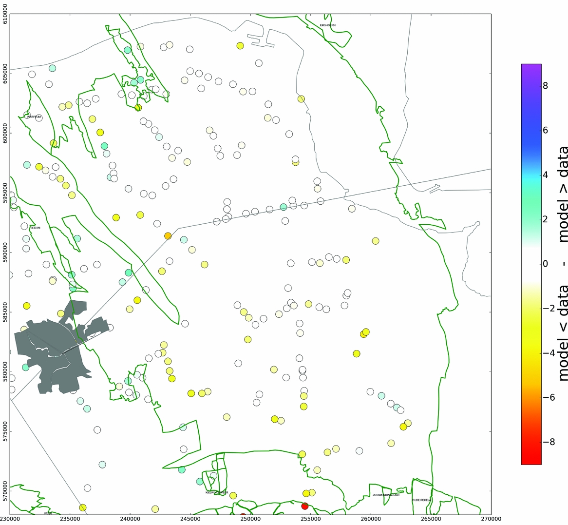
Fig. 11. Residuals map for the 1972–2013 period.
Next to the demonstration of the best fit, a methodology is also proposed to define the confidence range of the model, but it is mainly the uncertainty description of both model and data that can be improved. Fokker & van Thienen-Visser (Reference Fokker and Van Thienen-Visser2016) described the inversion of levelling double differences rather than using referenced absolute measurements to derive compaction. This method removes a possible geodetic bias that can be introduced by geodetic referencing processes. Van Thienen-Visser et al. (Reference Van Thienen-Visser, Pruiksma and Breunese2015) showed a first application of a particle-filtering method to more objectively determine which model performs best.
More recently a subsidence study for the Ameland field, executed by a NAM, TNO and TU-Delft consortium, leveraged on this existing knowledge by improving the uncertainty description of both models and data. The uncertainty in the data is described by a full variance/covariance matrix, and the application of a Bayesian particle-filtering technique foresees in the likelihood description of the subsurface realisations where the uncertainty both around reservoir models and geomechanical models is addressed (NAM 2017a,b).
Acknowledgements
We would like to express our very great appreciation to Dirk Doornhof and Harry Piening for their significant contribution to this paper. We are also grateful to Stijn Bierman for the improvements and discussions on the Groningen inversion workflows.


 Open access