


Introduction
It is well established that the climate during the ice ages was strongly influenced by the presence of large ice sheets on the continents of the Northern Hemisphere. A first coherent compilation of palaeoclimatic information was made in the 1970s by the CLIMAP (1976) project. Based on a multitude of geological and biological indicators, CLIMAP provided a geographical svnthesis of the world at the Last Glacial Maximum (LGM), which has been continuously updated and revised (Reference Frenzel, Peesi and VelichkoFrenzel and others, 1992). These studies are of great interest to a variety of modellers as they offer a number of essential boundary conditions for their models.
In large-scale ice-sheet modelling studies, however, it has proven difficult to simulate the three-dimensional (3-D) geometry of the Northern Hemisphere ice sheets so that results are in good agreement with the geological record (Reference Verbitsky and OglesbyVerbitsky and Oglesby, 1992; Reference MarsiatMarsiat, 1994; Reference HuybrechtsHuybrechts and T’siobbel, 1995). This defect is largely due to the inability of the models to prescribe correctly the surface mass-balance components of snow accumulation and meltwater runoff, but also due to inadequate modelling of basal conditions, ice rheology, and marine ice-sheet interactions. Crucial parameters for the determination of mass balance are meteorological variables such as air temperature, precipitation rate, circulation and energy Huxes al the ice surface. Ideally, such variables should arise from the interaction with complex general circulation models (GCMs). At present, however, models put a prohibitively high demand on computer resources that makes it impossible to couple them synchronously to 3-D ice-sheet models during a glacial cycle.
The 3-D climate model presented here represents an ellbrt to bridge the gap between an Iunergy Balance Model (EBM) and a complete GCM. The model is essentially a coarse-gridded GCM with simplified dynamics, which lakes into account the most important factors that are believed to influence the climate. Despite its relative simplicity, the climate model was shown to be able to simulate the present climate in reasonable agreement with observations (Reference SellersSellers, 1983, Reference Sellers1985a). Palaeoclimatic simulations different to the ones described here were conducted by Reference Sellers, Berger, Imbrie, Hays, Kukla and SaltzmanSellers (1985b) and Reference Friedlingstein, Delire, Müller and GerardFriedlingstein and others (1992).
The main purpose of this study is to investigate how well this model performs in predicting the change in climate between the LGM and the present day, and to investigate how these results can serve to prescribe boundary conditions for the modelling of the Northern Hemisphere ice sheets. Therefore, the climatic simulations are first compared with those obtained with more complex GCMs and subsequently used as input in a 3-D thermo-mechanical ice-sheet model (Reference HuybrechtsHuybrechts and T’siobbel, 1995). A comparison of ihe simulated ice-sheet configurations with the geological record then provides an indication about the quality and applicability of the climate model in ice-age-related studies.
The Climate Model
The quasi 3-D global climate model used in this stuck has been described in Reference SellersSellers (1983, Reference Sellers1985a, Reference Sellers, Berger, Imbrie, Hays, Kukla and Saltzmanb). It has a resolution of 10° × 10° and includes a complete hydroiogical cycle, a variable snow and ice cover, soil moisture, cloud cover, and an interactive ocean with diffusive heat transport but without currents. The principal equations that are solved in the model are conservation equations for energy and mass. There are five submodels associated with pressure and wind fields, moisture distribution, the radiation field, the surface water balance, and the temperature field.
The model has five vertical levels in sigma coordinates: three levels are in the troposphere and two are in the Stratosphere. The atmospheric flow in the lowest layer is assumed to depend on the Coriolis force, the pressure gradient and frictional forces, while the flow in the upper two tropospheric layers is geostrophic and determined by the t hernial wind equation. The only prognostic variables are the surface and 1 km temperature fields. The temperature lapse rate in the bottom layer is a function of the surface temperature, while the lapse rate in the two upper tropospheric layers is statistically related to the temperature at about 1 km, and is modified in order to preserve a radiation balance at the top of the atmosphere. These relatively simple dynamics allow a 5 day time-step.
An important simplification is made by setting the surface at sigma level = 1 (equal to sea level). This means that there are no explicit mountains in the model, which “feels” topography only through a surface drag coefficient that determines the friction of the continental surface on the wind in the lowest layer, and through the impact of elevation on the albedo-temperature feedback. Another simplification in the model includes the omission of acceleration terms in the calculation of wind speed, but this is justified for synoptic-scale phenomena.
The original papers (Reference SellersSellers, 1983, Reference Sellers1985a) demonstrate that the model is able to reproduce relatively well the present-day sea-level temperature and pressure fields. However, common to more complex GCMs, simulated precipitation patterns display dissimilarities with observations. For instance, the predicted precipitation is too high over North America and western Africa, and too low above 60°N, especially over the North Atlantic in winter.
The Simulated Climate of the LGM
To ensure consistency with the Palaeoclimate Modeling Intercomparison Project (PMIP) experiments, the LGM is assumed to have occurred at 21 000 BP. Thus, the orbital parameters, taken from Reference BergerBerger (1978), correspond to the situation al 21 OOO BP. The LGM as well as present-day (PD) topography is derived from Reference PeltierPeltier (1994). When compared with the PD topography, the number of continental points was increased by 25 for the LGM topography due to a glacioeustatic sea-level drop of about 105 m. This corresponds to an area of 12.8 × 10⁶ km2 of which most is situated in the high northern latitudes. The atmospheric CO2 concentration was reduced from 345 to 200 ppm for the LGM based on ice-core studies (Reference Barnola, Raynaud, Korotkevich and LoriusBarnola and others, 1987). There is no difference in the wax the albedo is treated in the climate model between the LGM and PD experiment: the albedo value over ice-sheet areas is set to 0.85, while that oxer snow is 0.75. The initial January conditions forsca-level temperature, snow, and sea-ice distributions for the present time were used in both the LCM and PD experiments.
To minimize the effect of systematic errors in the climate model, we concentrate on the difference between the LGM and PD climate. Model runs have been performed over 50 years with a 5 day time-step. The displayed runs are averaged oxer the last 5 years of the simulation.
Temperature
The simulated LGM annual global sea-level temperature is 2.1°C lower compared to that of the PD run. When we lake the effect of the LGM elevation into account, and apply a lapse rate for a cold and dry atmosphere of 8°C km−1 (e.g. Reference Hyde, Crowley, Kim and NorthHyde and others, 1989), the decrease in the LGM global annual surface temperature is 3.5°C. The global surface cooling is more pronounced during the summer months (JJA) (−4.3°C) than during winter (DJF) (−3.0°C), as it is (annually) over continent (−4.1°C) than over ocean (−1.6°C). The predicted global annual cooling relative to the PD corresponds quite well with values obtained by other, more complex, GCMs in LGM simulations (Kutz-bach and Guetter, 1986; Reference Broccoli and ManabeBroccoli and Manabe, 1987; Reference Lautenschlager and HerterichLautenschlager and Herterich, 1990; Reference JoussaumeJoussaume, 1993). Many GCMs also simulate a higher reduction of hemispheric air temperatures in summer than in winter, especially in the Northern Hemisphere (e.g. Reference Lautenschlager and HerterichLautenschlager and Herterich, 1990: Reference JoussaumeJoussaume, 1993).
The most prominent feature in Figure 1, which shows the simulated LGM minus PD change of sea-level temperature for different times of the year, is the intense cooling over the Northern Hemisphere ice sheets. The maximum annual cooling at sea level over the Laurentide ice sheet amounts to about 10°C, and is about 6°C over the Eurasian ice sheet. The cooling over the North Atlantic, however, is much smaller (about 3°C). A direct comparison between these results and those predicted by other GCMs is more difficult to make because the literature only provides surface temperatures, and different GCMs use different ice-sheet topographies and lapse rates. However, it seems that the annual results presented here are roughly in line for the Laurentide ice sheet, somewhat less for the Eurasian ice sheet, and substantially less for the North Atlantic. The latter is most probably caused by a poor modelling of the sea-ice distribution in the Sellers model and/or the use of a “too warm” initial sea-surface temperature dataset in the LGM experiment.
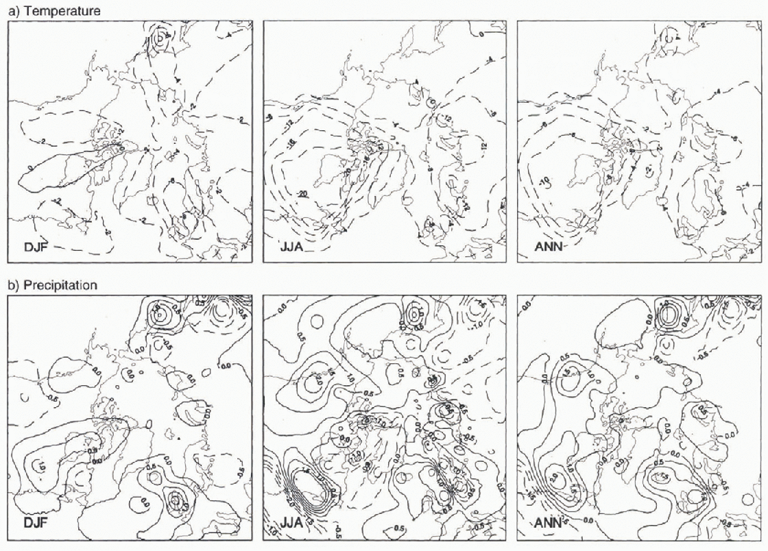
Fig. 1. Changes of sea-level temperature (a) and precipitation rate (b) as simulated by the climate model over a part of the. Northern Hemisphere. Shown are LGM minus present-day differences for the winter season (DJF), the summer season (JJA), and mean annual conditions (ANN), respectively. Units are in °C for temperature and mm d−1 for precipitation.
Another prominent feature of the simulations shown in Figure 1 is the very pronounced cooling simulated over both the Laurentide and Eurasian ice sheets during the summer months. This feature is also observed in the energy-balance model (EBM) simulations presented in Reference Hyde, Crowley, Kim and NorthHyde and others (1989), but is generally absent in GCM runs. Several GCM studies produce the largest cooling in summer over the Laurentide ice sheet (Reference Kutzbach and GuetterKutzbach and Guetter, 1986; Reference JoussaumeJoussaume, 1993), but over the North Atlantic and the Eurasian ice sheet, the largest cooling usually occurs during the winter months. Palaeodata also seem to be generally supportive of a larger cooling during winter than during summer in the vicinity of the large ice sheets at the LGM (e.g. Reference Frenzel, Peesi and VelichkoFrenzel and others, 1992), but conclusive evidence is lacking.
Precipitation
The precipitation rate in the climate model is obtained differently from that in the GCMs, where vertical moisture distribution is given by the continuity equation of water vapor. Here, the sum of the condensation and the vertical diffusion of moisture is calculated from the specific humid-ities at the top and bottom of each layer, and the moisture continuity equation for each tropospheric layer. It is assumed that when this sum is positive, a fraction condenses and the rest diffuses Vertically tO a higher layer. The total precipitation is then given by the sum of the condensate in each layer.
The model generally predicts reduced precipitation rates during the LGM. The annual mean precipitation rate over the entire globe is 7.5% lower than that for the PD simulation. This global reduction is stronger in summer (JJA) (−10%) than in winter (DJF) (−7%); and (annually) stronger over land (−11%) than over ocean (−6%). Again, these numbers are in qualitative agreement with those from most GCMs (e.g. Reference Kutzbach and GuetterKutzbach and Guetter, 1986), though they tend to be slightly lower.
However, there are also noticeable differences with other GCMs. The most important one is that the present model generally predicts a precipitation increase over the ice-sheet areas, whereas most GCMs, especially those with prescribed sea-level temperatures and sea-ice extent, simulate precipitation reductions over parts of the ice sheets (Reference Lautenschlager and HerterichLautenschlager and Herterich, 1990: Reference JoussaumeJoussaume, 1993). Possible explanations may be the present models low resolution or, alternatively, shortcomings in the calculation of the vertical temperature gradient over the ice sheets and/or the calculation of the horizontal moisture divergence. However, precipitation is a notoriously difficult process to model, and consensus amongst climate models remains doubtful.
The resulting annual mean and seasonal distributions of precipitation differences are presented in Figure 1. High precipitation changes occur in regions that are strongly influenced by differences in topography and/or circulation. The most prominent features in Figure 1 are the strong precipitation increases at the northwest and southeast sides of the Laurentide ice sheet and along the western side of the European ice sheet. These nodes, especially the one centered over Newfoundland, are a common feature in many simulations (Reference Broccoli and ManabeBroccoli and Manabe, 1987; Lauten-schlager and Herterich, 1990).
Circulation
In the model, topography influences atmospheric circulation in different ways. The first impact is that the surface wind is influenced by a surface drag coefficient that depends on elevation and wind speed. the second impact has a thermal origin in that the presence of an ice sheet induces a strong lowering of sea-level temperature through the albedo effect. This lower temperature changes the pressure at the surface level, as well as the position of the tropopause, and consequently influences the thickness of the troposphere (Reference SellersSellers, 1983). The resulting difference in horizontal pressure gradients is used in the wind equations, and therefore alter the atmospheric flow. Considering the assumptions made for the zonal and meridional winds, forcing for the LGM is primarily thermal in the climate model.
The winds at the 500 mb level are most indicative for large-scale circulation and are presented in Figure 2. Figure 2b shows that the planetary wave structure is strongly modified during the ice age, especially over North America. This forcing is primarily thermal. The presence of the huge Laurentide ice sheet curves the wind anticyclonically across northwestern North America. The northwesterlies associated with the downwind trough are channelled between the Laurentide and the Greenland ice sheets. The presence of the Laurentide ice sheet strengthens the westerly winds at its southern margin. The western North Atlantic jet is shifted towards the south, similar to what has been modelled by many GCMs (e.g. Reference JoussaumeJoussaume, 1993).
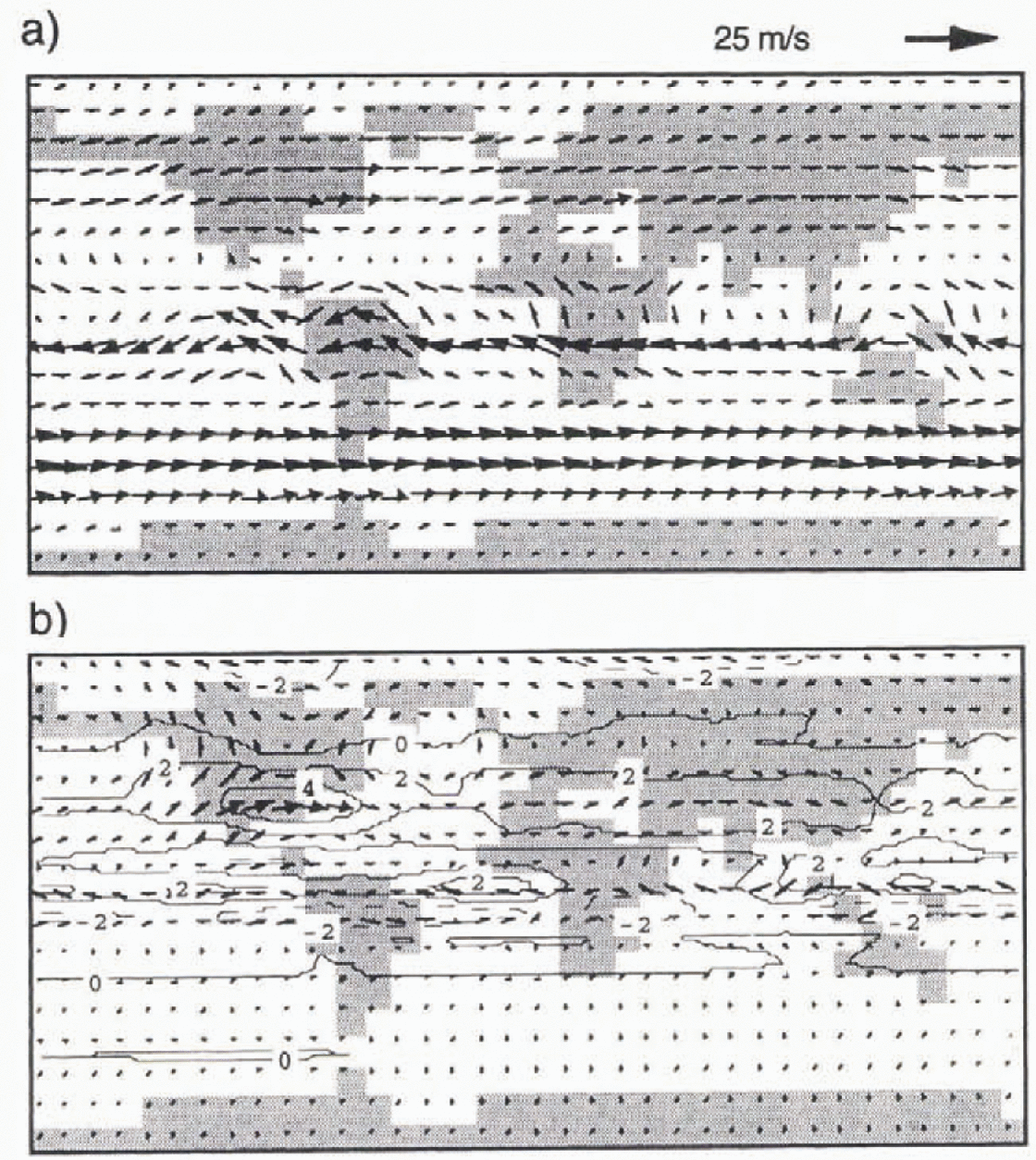
Fig. 2. The annual mean winds at the 500 mb level shown for the present-day simulation (a) and as the vector difference between the LGM and the present-day (b). The contours in (b) show the difference between LGM and present-day wind-speed magnitude (in m s−1). The arrow at the top provides a scale for the vectors.
A distint splitting of the jet stream as modelled by Reference Broccoli and ManabeBroccoli and Manabe (1987), on the other hand, is not simulated by our model. Reference Shinn and BarronShinn and Barron (1989) found that this bifurcation is strongly dependent on the type of ice-sheet reconstruction that is introduced as boundary condition in the GCMs. Awave ridge comparable to the one over the Laur-entide ice sheet is not simulated over northern Europe, and there is no prominent change in flow direction over Russia and Siberia. However, GCMs provide no consensus on the atmospheric circulation over Europe at the LGM. Lautens-chlager and Herterich (1990) found strong anticyclonic circulation associated with cold and dry norlheasterlies, while Reference JoussaumeJoussaume (1993) predicted storm tracks over Europe associated with strong westerlies and wetter conditions. The present model’s findings are closer to those of Reference JoussaumeJoussaume (1993).
Simulation of the Northern Hemisphere Ice Sheets
One way to assess the value and potential reality of the climatic simulations obtained above is to use the data in a numerical model of Northern Hemisphere ice sheets, because the resulting ice-sheet geometries can be independently compared with glacial-geological data. Such geological data usually constrain only the horizontal extent of the ice sheets, but further constraints on their thickness are provided by the interpretation of relative sea-level records around the globe (Reference PeltierPeltier, 1994). Having climatic data for only one moment in time, the ice-sheet simulations discussed below necessarily have to assume a stationary state. That may not have been the case in reality because of the long response times of ice sheels, but the effect is hard to quantify.
The ice-sheet model
The ice-sheet model used in this study was described in Reference HuybrechtsHuybrechts and T’siobbel (1995), with a full account of the model equations being given in Reference HuybrechtsHuybrechts (1993). It is a 3-D thermo-mechanical model, which includes bedrock adjustment, basal sliding and a full temperature calculation within the ice. The model has a horizontal mesh size of 50 km, 11 layers in the vertical, and covers all of the Northern Hemisphere where widespread continental glaciation is believed to have taken place. The model has been extensively tested and validated on the ice sheets of Greenland and Antarctica. However, unlike the Antarctic model, the model version employed here does not include a coupled ice shelf to enable a dynamic interaction with sea level, though grounded ice can still expand on the continental shelf as long as the surface mass balance allows it. All calculations take place on a square grid, which comprises 193 × 193 gridcells.
The main inputs to the model are bed topography, a mask specifying the maximum possible extent of grounded ice (following the −500 m isobath), mean annual surface temperature and the mass balance. The latter two represent climatic forcing. The inputs to the mass balance model are mean monthly surface temperature and mean monthly precipitation rates over the entire grid as specified below in Equations (1)–(5). The accumulation parameterisation takes into account the factor of precipitation falling as snow, which is determined by the surface temperature, and varies linearly from one to zero for mean monthly temperatures in the range of −10° to +7°C. Surface melting, which depends on the details of the energy fluxes at the ice-atmosphere interface, is better determined locally than is possible on the coarse grid of a climate model or GCM. Therefore, following Reference ReehReeh (1991), the melting rate is set as proportional to the yearly sum of positive degree days (PDD) at the surface. Degree-day factors were set at 3.5 mm a−1 PDD−1 for snow and 7 mm a−1 PDD−1 for ice. The model furthermore incorporates the process of superimposed ice formation, but neglects a possible contribution from rainfall, which is assumed to run off entirely.
The coupling scheme
The mass-balance model was forced by making use of the mean monthly sea-level temperature and precipitation-rate data from the LGM and PD climatic simulations described above. This requires the interpolation of the climatic data to the 50 km grid employed in the ice-sheet model. Because of the coarse 10° × 10° resolution of the climate model, and the resulting poor representation of topography, it is not meaningful to use absolute values of climate variables. Instead, we chose lo superimpose mean monthly changes of both sea-level temperature and precipitation rate LGM minus PD) upon the reference climatologies used by the mass-balance model. These were taken from precipitation maps (Reference JaegerJaeger, 1976) and from temperature data used to initialize the Hamburg GCM model (ECHAM-1 in the T21 mode) at the 1000 hPa level.
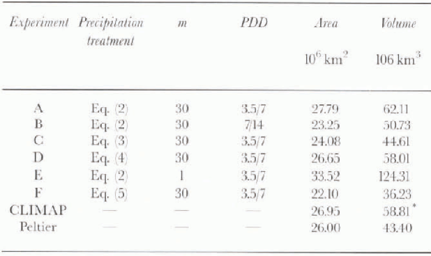
Altogether, we considered six different ice-sheet experiments, denoted Experiments A to F. These aimed primarily to investigate the optimal formulation of the interface between the climate and the ice-sheet model and to examine the role of changes in the melt model (Experiment B), the role of changes in the precipitation treatment (Experiments C and F), and the effect of using flow-law parameters appropriate for the Greenland ice sheet (Experiment E). Table 1 provides an overview of the various model setups used in these experiments.
Table 1. Summary of the ice-sheet experiments showing the mode! parameters and the simulated area and volume of the,Northern Hemisphere ice sheets at the LGA1. m is an en-hancement factor i n Glen's flow law; PDD are the degree- dayfactors for snow and ice melting, respectively. * represents ice volume, derived from the surface elevation data shown in Figure 3, assuming local isostatic equilibrium and an ice mantle rock density ratio of 0.275
All experiments were forced by mean monthly temperature anomalies resulting from the climate model as follows:
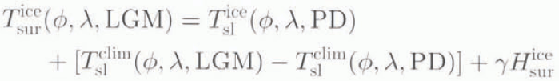
where T is mean monthly temperature (in °C),
H is elevation (in m), γ is the adopted atmospheric
lapse rate over ice sheets (8°C km−1),ϕ and λ are geographic
coordinates, “PD” and “LGM” refer to the time, the subscripts “sur” is for
surface and “sl” is for sea level, and the superscripts “ice” refer to the
ice-sheel model and “dim” to the climate model.
![]() (ϕ, λ, present) is the present monthly mean sea-level
temperature taken from the reference climatology.
(ϕ, λ, present) is the present monthly mean sea-level
temperature taken from the reference climatology.
Changes in precipitation rate are more difficult to handle because of the large uncertainties in the model simulations. Therefore, four different treatments were tested. In the standard approach, we superimposed the ratio of precipitation intensities as resulting from the climate model on the PD data for the mean monthly precipitation rate in the mass balance model:
where pice(ϕ, λ, PD) is the mean monthly precipitation rate (m a−1) as taken from the reference climatology, and superscripts are the same as in Equation (1).
An alternative approach, used in Experiment C, set the precipitation rate proportional to the moisture-holding capacity of an air column with a sensitivity of 4% °C−1, similar to the approach taken in Reference HuybrechtsHuybrechts and T’siobbel (1995):
In the third approach (Experiment D), the standard approach was modified to take into account absolute precipitation differences between the LGM and the PD climatic simulations rather than precipitation ratios:

Finally, in Experiment F, an elevation-desert effect was introduced by relating the precipitation intensity to the change in surface temperature rather than to the change in sea-level temperature:
Results
All experiments were run for 50 00 years, when an approximate steady state set in. The resulting ice-sheet geometries are presented in Figure 3, with the corresponding values for the ice-sheet area and ice volume shown in Table I, Overall, the ice-sheel model is able to produce reasonable results, which compare well with the independent reconstructions given in the bottom panels. In Experiments A-D, the resulting values for ice-covered areas are all within 10% of the glacial-geological reconstructions, and the resulting ice volumes fall within the bracket given by both the Reference PeltierPeltier (1994) and CLIMAP (1976) reconstructions. In Experiment A, the Laurentide ice sheet has approximately the right configuration, including a correct simulation of the ice-free areas in northern Alaska. The Eurasian ice sheet, on the other hand, fails to reach the southern shores of the Baltic Sca and extends too far to the south along the Ural Mountains. The latter is probably due to the coarse resolution of the climate model, which indicates a too-large cooling in that area. Except for Experiment E, none of the model simulations shows a connection between the Scandinavian and British ice sheets, but here both the Reference PeltierPeltier (1994) and CLIMAP (1976) reconstructions disagree.
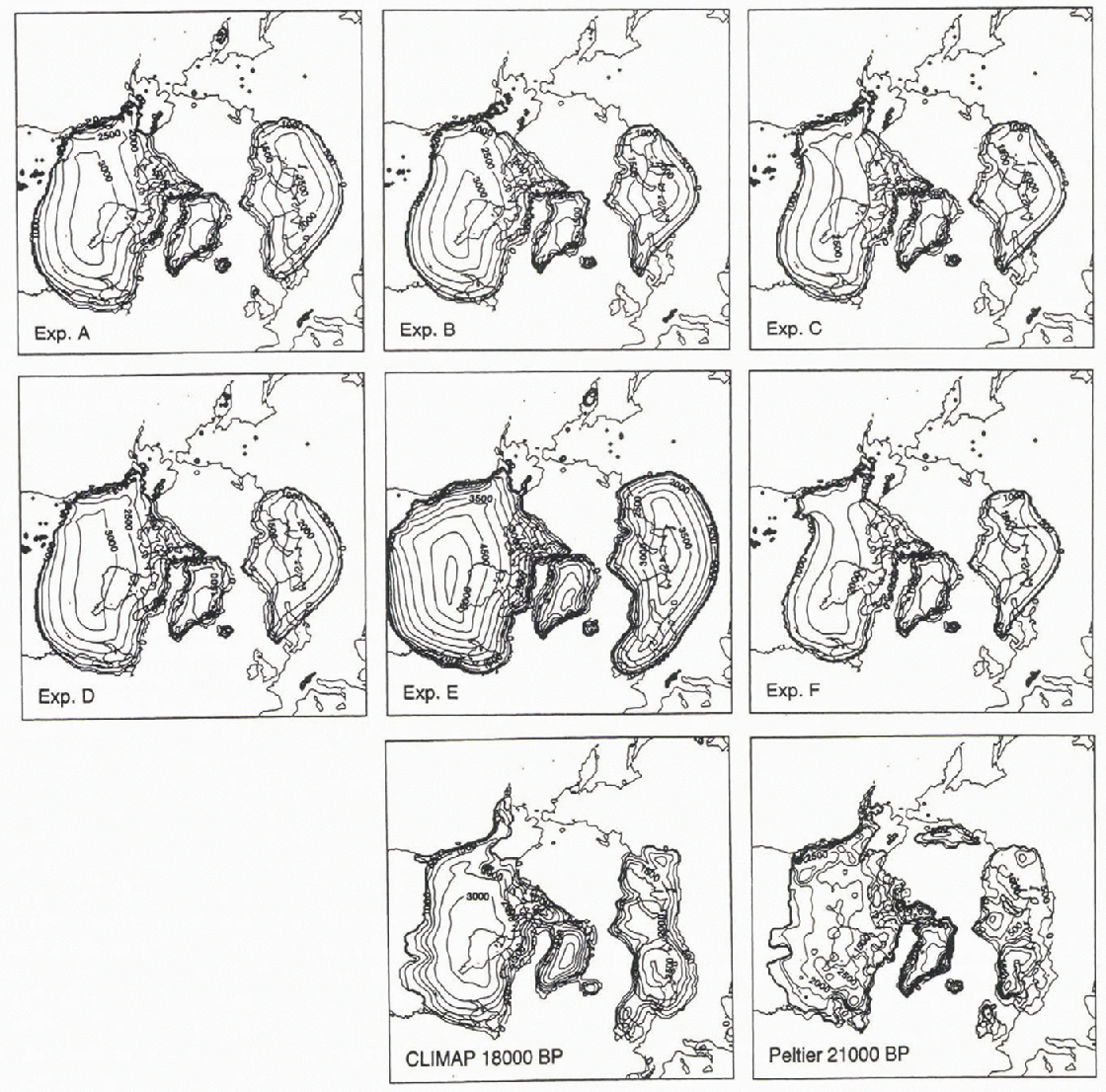
Fig. 3. Simulated steady-state geometries of the Northern Hemisphere ice sheets at the LGM using output from the climate model as explained in the text (Experiments A-F). For comparison, the bottom panels show the glacial—geological reconstruction from the CLIMAP (1976) project and of a more recent reconstruction derived from a gravitational theory of postglacial relative sea-level change (Reference PeltierPeltier, 1994).
Given the climatic input as Specified above, the ice-sheet model has two tuning possibilities. The degree-day factors in the melting model primarily influence the width and extent of the ice sheets, but it was not necessary to change these factors from the standard values measured in central west Greenland (Reference Braithwaite, Olesen and OerlemansBraithwaite and Olesen, 1989). The effect of doubling these factors, which is still within their range of uncertainty, is shown by comparing Experiment A with Experiment B. In the latter, the ice sheets retreat at their southern margins, and ice volume and surface area diminish by about 18%.
Another important tuning parameter is a multiplier in the rate factor of Glen’s flow law, which primarily determines the height-to-width ratio. In order to get the maximum height and total ice volume within reasonable bounds, it was necessary to use an enhancement factor of 30 with respect to previous simulations of the Greenland ice sheet using the same flow law (Reference Huybrechts, Letréguilly and ReehHuybrechts and others, 1991). The effect is demonstrated in Experiment E, which shows results obtained for an enhancement factor of 1. That produces a much more reasonable surface elevation over central Greenland, but makes the Laurentide and Fenno-scandian ice sheets thicker by about 50%. This is because mean ice thickness is at first approximation proportional to the rate factor to the power −1/8 (Reference PatersonPaterson, 1994), and because the surface area also increases by about a third. The implication seems to be that the ice in the Laurentide and Fennoscandian ice sheets was either a lot softer, and thus deformed more easily, or that the ice-sheet beds allowed for more sliding.
An indication of the latter may be the absence in the model of the two distinct lobes that stretch out into the mid-western U.S.A., which are often attributed to the presence of soft layers of deformable till in the area of the Great Lakes (Reference ClarkClark, 1994). The surface topography of the Laurentide ice-sheet, on the other hand, does not support the Reference PeltierPeltier (1994) reconstruction in most of our simulations, which shows many different domes and a central elevation of between 2000 and 2500 m only. However, two separate domes, centered over the Rockies and eastern Canada, emerge when reduced precipitation rates are applied (Experiments C and F). Provided the Reference PeltierPeltier (1994) reconstruction is preferred over the CLlMAP (1976) reconstruction, this seems to indicate that precipitation rates at the LGM might have been significantly lower than at present, unlike the results from the climate model.
The introduction of an additional desert-elevation effect (Experiment F), on the other hand, which produces even drier conditions over the Northern Hemisphere ice sheets similar to those presently prevailing over Antarctica, leads to ice sheels that become too thin with respect to the geological reconstructions. Finally, applying precipitation differences (Experiment D) rather than precipitation ratios (Experiment A) does not make much difference to the results.
Compared to previous simulations of Northern Hemisphere ice sheets (Reference Deblonde and PeltierDeblonde and Peltier, 1991; Reference Verbitsky and OglesbyVerbitsky and Oglesby, 1992; Reference MarsiatMarsiat, 1994; Reference HuybrechtsHuybrechts and T’siobbel, 1995), the major improvement in the present simulations is the absence of large ice sheets in northern Alaska and northeastern Siberia. This is mainly a consequence of the climatic forcing.
Conclusions
In this study, we have investigated the application of a 3-D climate model, intermediate between an EBM and a full GCM, to prescribe boundary conditions for the modelling of Northern Hemisphere ice sheets. It was demonstrated that many aspects of the climate predicted for the LGM appeared very reasonable and agreed well with those produced by more complex GCMs, except for the small cooling over the North Atlantic, the larger cooling predicted for the summer rather than for the winter, and the general increase of precipitation over the Laurentide ice sheet. These effects could be due to the low resolution of the climate model or, alternatively, to deficiencies in the sea-ice model, the hydro-logical cycle, or the way the circulation reacts to the presence of ice sheets. Conclusive field evidence to test the model is lacking.
Nevertheless, despite the simplifications applied during the climate model runs, it was shown that using the resulting temperature and precipitation anomalies in a 3-D mass balance and ice-sheet model led to reasonable configurations of the LGM ice sheets. This could be seen as an indication that the climate model may well have captured the most essential characteristics of the LGM climate, and thus provides a useful forcing for the prescription of the surface mass balance of the Northern Hemisphere ice sheels at the LGM. The logical step forward would be to feed the information of the ice-sheet model back into the climate model, and subsequently try to simulate a whole cycle of ice-sheet advance and retreat. With present-day computer resources, the coupled 3-D climate ice-sheet model would enable simulation of such a scenario in an interactive way.
Acknowledgements
This paper is a contribution to the Belgian Impulse Programme on Global Change, initiated by the Federal Office for Scientific, Technical and Cultural Affairs (Services of the Prime Minister). During this research, P. Huybrechts was supported by the Belgian National Fund for Scientific Research (NFWO). We thank W. D. Sellers for the use of his climate model.


