


1. Introduction
A century ago, Zeleny (Reference Zeleny1917) photographed instabilities of electrified interfaces, sparking interest into understanding the phenomenon. The mechanisms of interface destabilization by electric fields have been studied in the pioneering works of Taylor (Reference Taylor1964), Taylor & McEwan (Reference Taylor and McEwan1965) and Melcher and coworkers (Melcher & Schwarz Reference Melcher and Schwarz1968; Melcher & Smith Reference Melcher and Smith1969), followed by an extensive body of research aimed at gaining more detailed fundamental understanding and at exploiting electrohydrodynamic (EHD) instabilities in novel applications (Melcher & Taylor Reference Melcher and Taylor1969; Saville Reference Saville1997; Griffing et al. Reference Griffing, Bankoff, Miksis and Schluter2006; Barrero & Loscertales Reference Barrero and Loscertales2007; Fernández de La Mora Reference Fernández de La Mora2007; Wu & Russel Reference Wu and Russel2009; Basaran, Gao & Bhat Reference Basaran, Gao and Bhat2013; Ganan-Calvo et al. Reference Ganan-Calvo, López-Herrera, Herrada, Ramos and Montanero2018; Papageorgiou Reference Papageorgiou2019; Vlahovska Reference Vlahovska2019).
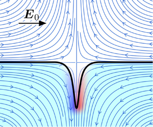
Interfaces polarize in applied electric fields. Free charges brought by conduction accumulate at the boundary between phases and the electric field acting on this induced charge creates shear stresses that drag the fluids into motion (Melcher & Taylor Reference Melcher and Taylor1969). In the case of a drop in a uniform electric field, the classic small-deformation analysis by Taylor (Reference Taylor1966) showed that the resulting EHD flow consists of two toroidal vortices inside and a stresslet-quadrupole flow outside the drop. Depending on the electric properties of the fluids, the surface flow is directed either to the poles or to the equator. The latter case is shown in figure 1(a). In strong fields, however, this flow undergoes a plethora of instabilities that may result in drop breakup (Taylor Reference Taylor1964; Torza, Cox & Mason Reference Torza, Cox and Mason1971; Sherwood Reference Sherwood1988; Lac & Homsy Reference Lac and Homsy2007; Karyappa, Deshmukh & Thaokar Reference Karyappa, Deshmukh and Thaokar2014). Droplet disintegration can proceed in various patterns depending on fluid properties. In the case of the pole-convergent flow, the drop can develop conical tips that emit jets, which subsequently break up into droplets (Collins et al. Reference Collins, Jones, Harris and Basaran2008, Reference Collins, Sambath, Harris and Basaran2013; Mohamed et al. Reference Mohamed, Lopez-Herrera, Herrada, Modesto-Lopez and Ganan-Calvo2016; Sengupta, Walker & Khair Reference Sengupta, Walker and Khair2017). In the case of the equator-converging flow, the drop either dimples at the poles and breaks into a torus, or deforms into a pancake-like lenticular shape with a sharp edge emitting rings encircling the drop (Brosseau & Vlahovska Reference Brosseau and Vlahovska2017; Wagoner et al. Reference Wagoner, Vlahovska, Harris and Basaran2020).

Figure 1. An oblate drop under a uniform electric field. ( $a$) The quadrupolar EHD flow from the poles to the equator. ( $b$) Convergent streamlines and tangential electric field in the vicinity of the stagnation line.
While EHD streaming from Taylor cones has been extensively studied (Collins et al. Reference Collins, Jones, Harris and Basaran2008, Reference Collins, Sambath, Harris and Basaran2013; Herrada et al. Reference Herrada, López-Herrera, Gañán Calvo, Vega, Montanero and Popinet2012; Ganan-Calvo et al. Reference Ganan-Calvo, López-Herrera, Rebollo-Munoz and Montanero2016), the mechanisms underlying the equatorial streaming remain an open question. Noting the similarity between the EHD tip streaming and the tip streaming in flow focusing (Barrero & Loscertales Reference Barrero and Loscertales2007; Ganan-Calvo & Montanero Reference Ganan-Calvo and Montanero2009; Anna Reference Anna2016), Brosseau & Vlahovska (Reference Brosseau and Vlahovska2017) speculated, in the original paper that reported the phenomenon, that the EHD equatorial streaming arises from an interfacial instability due to a convergent flow (Pozrikidis & Blyth Reference Pozrikidis and Blyth2004; Blyth & Pozrikidis Reference Blyth and Pozrikidis2005; Tseng & Prosperetti Reference Tseng and Prosperetti2015). Near a stagnation point, a perturbation of the interface may get drawn by the flow and grow into a fluid filament if viscous stresses overcome interfacial tension. Unlike flow focusing, however, EHD streaming involves both flow and electric field. In EHD tip streaming, the electric field is initially normal to the interface at the stagnation point, while in EHD equatorial streaming, the applied field is parallel to the interface at the stagnation line.
In this work, we analyse the effect of an electric field on the convergent flow instability in a configuration mimicking the EHD equatorial streaming as depicted in figure 1( $b$). We develop a two-dimensional model to study the dynamics of a system of two superimposed layers of fluids subject to a tangential electric field and a stagnation point flow. The convergent flow and the electric field are assumed to be independently applied, unlike the equatorial EHD instability, where the flow is generated by the electric field. Despite this simplification, the analysis provides valuable insights into mechanisms responsible for the EHD equatorial streaming such as the evolution of the convergent line instability and the emergence of charge shocks. We present the governing equations in § 2 and their non-dimensionalization in § 3. We develop a local linear stability theory in § 4. To supplement our theory, we employ the boundary element method, outlined in § 5, to perform numerical simulations as well as a numerical linear stability analysis. We compare the results from the local theory, numerical linear stability analysis and transient simulations in § 6. Finally, we conclude and discuss potential extensions of this work in § 7.
2. Problem definition and governing equations
We study EHD instabilities that arise at the interface  $S$ between two immiscible fluids under the combined effects of a tangential electric field $\boldsymbol {E}_0$ and of an imposed stagnation point flow $\boldsymbol {u}^{\infty }(\boldsymbol {x})$, to be specified more precisely later. The two layers are labelled 1 and 2 as depicted in figure 2, with fluid 1 occupying the lower half-space. The applied electric field is uniform along the $x$ direction, and the stagnation point is located on the interface at the origin $O$ of the coordinate system. At equilibrium, the interface is uncharged and flat and coincides with the plane $z=0$, and we consider two-dimensional dynamics in the $(x,z)$ plane. The shape of the deformed interface is parametrized as $z=\xi (x,t)$, and has unit normal $\boldsymbol {n}$ pointing from fluid 1 into fluid 2.

Figure 2. Problem definition. Two immiscible fluid layers are subject to a tangential electric field  $\boldsymbol {E}_0$ and to a planar extensional flow $\boldsymbol {u}^{\infty }(\boldsymbol {x})$, with a stagnation point located at the origin $O$ on the interface.
Both fluids are leaky dielectrics with electric conductivity  $\sigma$, electric permittivity $\epsilon$ and dynamic viscosity $\mu$. While we formulate the governing equations to allow for distinct viscosities, all the results presented in § 6 are for equiviscous fluids. Under the Taylor–Melcher leaky dielectric model (Melcher & Taylor Reference Melcher and Taylor1969), any net charge in the system occurs at the location of the interface while the bulk of the fluids remains electroneutral. The Taylor–Melcher leaky dielectric model can be formally derived from more detailed electrokinetic models based on the Poisson–Nernst–Planck equations in the limit of strong electric fields and under the assumption of thin Debye layers (Schnitzer & Yariv Reference Schnitzer and Yariv2015; Mori & Young Reference Mori and Young2018). As an example, these assumptions are valid for millimetre-sized drops of leaky dielectric liquids subject to electric fields of magnitude $E_0\sim 10^3$ V cm $^{-1}$ according to Saville (Reference Saville1997). Under these assumptions, the electric potential is harmonic in both fluids:
 \begin{equation} \nabla^2 \varphi=0,\quad \boldsymbol{x}\in V_{1,2}. \end{equation}
Far from the interface, the electric field  $\boldsymbol {E}=-\boldsymbol {\nabla }\varphi$ tends to the applied uniform field:
 \begin{equation} \boldsymbol{E}\rightarrow \boldsymbol{E}_0=E_0 \hat{\boldsymbol{e}}_x, \quad \text{as } z\rightarrow \pm \infty. \end{equation}
Across the interface, its tangential component is continuous while a jump can arise in the normal direction due to the mismatch in electrical properties:
 \begin{equation} \boldsymbol{n} \times [\![ \boldsymbol{E} ]\!]=\boldsymbol{0},\quad \boldsymbol{x}\in S.\end{equation}
We have introduced the notation  $[\![ \mathcal {F} ]\!]=\mathcal {F}_2-\mathcal {F}_1$ for the jump of any variable $\mathcal {F}$ defined on both sides of the interface. A surface charge density develops at the interface following Gauss's law:
 \begin{equation} q(\boldsymbol{x},t)=\boldsymbol{n}\boldsymbol{\cdot}[\![ \epsilon \boldsymbol{E} ]\!],\quad \boldsymbol{x} \in S. \end{equation}
This surface charge density satisfies a conservation equation accounting for finite charge relaxation, Ohmic conduction from the bulk and charge convection by the flow:
 \begin{equation} \partial_t q+\boldsymbol{n}\boldsymbol{\cdot}[\![ \sigma \boldsymbol{E}]\!] + \boldsymbol{\nabla}_{ s} \boldsymbol{\cdot}(q \boldsymbol{u})=0,\quad \boldsymbol{x}\in S, \end{equation}
where  $\boldsymbol {\nabla }_{ s}= ({\boldsymbol{\mathsf{I}}}-\boldsymbol {n}\boldsymbol {n})\boldsymbol {\cdot }\boldsymbol {\nabla }$ is the surface gradient operator and $\boldsymbol {u}$ is the total fluid velocity.
Neglecting the effects of inertia and gravity, the velocity field and its corresponding pressure field satisfy the Stokes equations in both fluids:
 \begin{equation} -\boldsymbol{\nabla} p+\mu \nabla^2\boldsymbol{u}=\boldsymbol{0}, \quad \boldsymbol{\nabla}\boldsymbol{\cdot}\boldsymbol{u}=0,\quad \boldsymbol{x}\in V_{1,2}. \end{equation}
The velocity vector is continuous across the interface and approaches the applied flow far from the interface:
 \begin{equation} [\![ \boldsymbol{u} ]\!]=\boldsymbol{0},\quad \boldsymbol{x}\in S, \end{equation}
and
 \begin{equation} \boldsymbol{u}(\boldsymbol{x})\rightarrow \boldsymbol{u}^{\infty}(\boldsymbol{x}), \quad \text{as } z\rightarrow \pm \infty . \end{equation}
In the absence of Marangoni effects, the jump in hydrodynamic and electric tractions across the interface is balanced by capillary forces:
 \begin{equation} [\![ \boldsymbol{f}^H]\!] + [\![ \boldsymbol{f}^E]\!]=\gamma (\boldsymbol{\nabla}_{ s}\boldsymbol{\cdot} \boldsymbol{n})\boldsymbol{n},\quad \boldsymbol{x}\in S,\end{equation}
with uniform surface tension  $\gamma$. Hydrodynamic and electric tractions are expressed in terms of the Newtonian and Maxwell stress tensors, respectively:
 \begin{gather} \boldsymbol{f}^H=\boldsymbol{n}\boldsymbol{\cdot}{\boldsymbol{\mathsf{T}}}^H,\quad {\boldsymbol{\mathsf{T}}}^H={-}p{\boldsymbol{\mathsf{I}}}+\mu(\boldsymbol{\nabla}\boldsymbol{u}+{\boldsymbol{\nabla}\boldsymbol{u}}^T), \end{gather}
 \begin{gather}\boldsymbol{f}^E=\boldsymbol{n}\boldsymbol{\cdot}{\boldsymbol{\mathsf{T}}}^E, \quad {\boldsymbol{\mathsf{T}}}^E=\epsilon (\boldsymbol{E}\boldsymbol{E} -\tfrac{1}{2}E^2{\boldsymbol{\mathsf{I}}}). \end{gather}
Finally, the interface evolves and deforms under the local velocity field as a material surface. Defining the function  $g(\boldsymbol {x},t)=z-\xi (x,t)$, the kinematic boundary condition reads
 \begin{equation} \frac{\mathrm{D}g}{\mathrm{D}t}=0, \quad \boldsymbol{x}\in S, \end{equation}
leading to the condition
 \begin{equation} \partial_t \xi ={-}u \partial_x \xi + v, \end{equation}
where  $\boldsymbol {u}=(u,v)$ are the velocity components. We also note that the surface normal is given by $\boldsymbol {n}=\boldsymbol {\nabla } g/|\boldsymbol {\nabla } g|$.
Our focus is on analysing the stability of the interface near a stagnation point, and to this end we choose the background flow  $\boldsymbol {u}^{\infty }=(u^{\infty },v^{\infty })$ to be extensional along the $z$ direction, compressional along the $x$ direction and with a stagnation point at the origin. The strength of the background flow is characterized by the local strain rate at the stagnation point, which is denoted by $A=\partial _z v^{\infty }$, where $A>0$. Three different types of background flows are used in this study and are illustrated in figure 3. The first type, depicted in figure 3( $a$), is simply the linear flow $\boldsymbol {u}^\infty =(-Ax,Az)$, which is used in the development of the local linear theory of § 4. The numerical scheme of § 5, however, requires periodicity in the $x$ direction, and for this reason we also consider two periodic flow fields. The first one is the Taylor–Green vortex (Taylor & Green Reference Taylor and Green1937) shown in figure 3( $b$) and defined as
 \begin{gather} u^{\infty}=U^{\infty} \cos\left(a x-\frac{\rm \pi}{2}\right) \sin\left(b z-\frac{\rm \pi}{2}\right), \end{gather}
 \begin{gather}v^{\infty}=V^{\infty} \sin\left(a x-\frac{\rm \pi}{2}\right) \cos\left(b z-\frac{\rm \pi}{2}\right), \end{gather}
where
 \begin{equation} U^{\infty} a+ V^{\infty}b =0, \quad a=b=\frac{2{\rm \pi}}{L_p}.\end{equation}
The local strain rate at the stagnation point is then simply given by
 \begin{equation} A=\partial_z v^{\infty}(0,0)= V^{\infty}b. \end{equation}
We also consider a second background flow shown in figure 3( $c$) and induced by a periodic array of anti-parallel point forces separated by distances $L_p$ and $d$ along the $x$ and $z$ directions, respectively:
 \begin{equation} \boldsymbol{u}^{\infty}=\frac{1}{4 {\rm \pi}} [ {\boldsymbol{\mathsf{G}}}^P(\boldsymbol{x},\boldsymbol{x}_0^u) \boldsymbol{\cdot} \boldsymbol{m}-{\boldsymbol{\mathsf{G}}}^P(\boldsymbol{x},\boldsymbol{x}_0^l)\boldsymbol{\cdot} \boldsymbol{m} ],\end{equation}
where  $\boldsymbol {m}=m\boldsymbol {\hat {e}_z}$ is the strength of the point forces, $\boldsymbol {x}_0^u$ and $\boldsymbol {x}_0^l$ are the locations of upper and lower point forces, respectively, and ${\boldsymbol{\mathsf{G}}}^P$ is the singly periodic Green's function for the Stokes equations (Pozrikidis Reference Pozrikidis1992). The local strain rate at the stagnation point is given by
 \begin{equation} A=\partial_z v^{\infty}(0,0)=\frac{1}{8{\rm \pi}} \left( \frac{m k_p^2 d }{\cosh{ ( k_p d/2 ) }-1} \right),\end{equation}
where  $k_p=2{\rm \pi} /L_p$ is the wavenumber associated with the unit cell. In obtaining (2.19), it is assumed that $x^u_0=x^l_0=0$ and $z^u_0=-z^l_0=d/2$. Our numerical calculations produce identical linear stability results for a given local strain rate under the two periodic flow fields described by (2.15) and (2.18). In all transient nonlinear simulations, we use the periodic array of point forces as background flow.

Figure 3. Streamlines of the various background flows used in this study. ( $a$) Linear planar extensional flow, ( $b$) periodic Taylor–Green vortex and ( $c$) periodic array of anti-parallel point forces separated by $d$ and $L_p$ along the $z$ and $x$ directions, respectively. The origin is marked with a ‘+’, the positions of the point forces are marked with triangles and the interface is located at $z=0$.
3. Non-dimensionalization
For the system presented above, dimensional analysis yields six non-dimensional groups, three of which characterize the mismatch in physical properties between the two layers:
 \begin{equation} \lambda=\frac{\mu_1}{\mu_2}, \quad R=\frac{\sigma_2}{\sigma_1}, \quad Q=\frac{\epsilon_1}{\epsilon_2}. \end{equation}
The other three parameters can be obtained as ratios of characteristic time scales in the problem. First, we note that free charges in the bulk fluids relax on a conduction time scale defined as
 \begin{equation} \tau_c=\frac{\epsilon}{\sigma}. \end{equation}
Note that the product  $RQ=\tau _{c,1}/\tau _{c,2}$ is the ratio of the charge relaxation time scales in the two liquid phases, and characterizes their responses to conduction. For instance, $RQ>1$ when the lower layer is less conductive. The time scale for the deformed interface to relax to its flat configuration under capillary effects can be defined as
 \begin{equation} \tau_{\gamma}=\frac{\mu_2(1+\lambda)}{k \gamma}, \end{equation}
where  $k^{-1}$ is the characteristic length scale associated with the deformation. In our periodic simulations and analysis, we use the length scale $k_p^{-1}=L_p/2{\rm \pi}$ based on the periodicity of the base flow, whereas $k$ is the wavenumber of the plane wave in the local stability theory of § 4. The accumulation of free charges on the interface creates an electric force that can drive the fluid into motion. The time scale for deformations under this EHD flow is inversely proportional to the magnitude of electric tractions on the interface:
 \begin{equation} \tau_{_{EHD}}=\frac{\mu_2 (1+\lambda)}{\epsilon_2 E_0^2}. \end{equation}
Finally, the characteristic time scale associated with the background flow is given by the inverse of the applied strain rate at the stagnation point:
 \begin{equation} \tau_{f}=A^{{-}1}. \end{equation}
Taking ratios of these time scales yields the three remaining dimensionless groups, which we define as
 \begin{equation} Ca_E=\frac{\tau_{\gamma}}{\tau_{_{EHD}}}=\frac{\epsilon_2 E_0^2}{\gamma k}, \quad Re_E=\frac{\tau_{c,2}}{\tau_{_{EHD}}}=\frac{\epsilon_2^2 E^2_0}{\mu_2(1+\lambda)\sigma_2}, \quad \hat{A}=\frac{\tau_{c,2}}{\tau_f}=\frac{\epsilon_2 A}{\sigma_2}.\end{equation}
The electric capillary number  $Ca_E$ compares electric with capillary forces, while the electric Reynolds number $Re_E$ characterizes the importance of charge convection versus conduction, the two mechanisms responsible for the evolution of the interfacial charge distribution. Finally, $\hat {A}$ is the dimensionless strain rate of the applied flow.
We scale the governing equations and boundary conditions using time scale  $\tau _{c,2}$, length scale $k^{-1}$, pressure scale $\epsilon _2 E^2_0$, velocity scale $(\tau _{EHD}k)^{-1}$ and characteristic electric potential $E_0 k^{-1}$. The dimensionless Stokes equations read
 \begin{align} \nabla^2\boldsymbol{u} -(1+\lambda) \boldsymbol{\nabla} p=\boldsymbol{0}, \quad \boldsymbol{x}\in V_{2}, \end{align}
 \begin{align} \nabla^2\boldsymbol{u} -({1+\lambda^{{-}1}}) \boldsymbol{\nabla} p=\boldsymbol{0}, \quad \boldsymbol{x}\in V_{1}. \end{align}
The charge conservation equation (2.5) becomes
 \begin{equation} \partial_t q+ \boldsymbol{n} \boldsymbol{\cdot} [ \boldsymbol{E}_2-R^{{-}1} \boldsymbol{E}_1 ] + Re_E\boldsymbol{\nabla}_{ s} \boldsymbol{\cdot} (q\boldsymbol{u})=0,\quad \boldsymbol{x}\in S, \end{equation}
where
 \begin{equation} q= \boldsymbol{n} \boldsymbol{\cdot} [\boldsymbol{E}_2- Q\boldsymbol{E}_1]. \end{equation}
The stress balance at the interface is written
 \begin{align} &\boldsymbol{n} \boldsymbol{\cdot} [{-}p_2{\boldsymbol{\mathsf{I}}}+(1+\lambda)^{{-}1}(\boldsymbol{\nabla}\boldsymbol{u}_2+\boldsymbol{\nabla}\boldsymbol{u}_2^T) +p_1{\boldsymbol{\mathsf{I}}}-(1+\lambda^{{-}1})^{{-}1}(\boldsymbol{\nabla}\boldsymbol{u}_1 +{\boldsymbol{\nabla}\boldsymbol{u}}^T_1)]\nonumber\\ &\quad +\boldsymbol{n} \boldsymbol{\cdot} \big[(\boldsymbol{E}_2\boldsymbol{E}_2 -\tfrac{1}{2}E_2^2{\boldsymbol{\mathsf{I}}})-Q (\boldsymbol{E}_1\boldsymbol{E}_1 -\tfrac{1}{2}E^2_1{\boldsymbol{\mathsf{I}}}) \big]=Ca_E^{{-}1} (\boldsymbol{\nabla}_{ s} \boldsymbol{\cdot} \boldsymbol{n})\boldsymbol{n},\quad \boldsymbol{x}\in S. \end{align}
Finally, the kinematic boundary condition becomes
 \begin{equation} \partial_t \xi =Re_E ({-}u\partial_x \xi+v), \quad \text{for }\boldsymbol{x}\in S.\end{equation}
The remaining governing equations and boundary conditions in (2.1)–(2.3), (2.7) and (2.8) remain unchanged in their non-dimensional form, and hence are not repeated here. In the remainder of the paper, all equations and variables are presented in non-dimensional form.
4. Local linear stability theory
We first perform a linear stability analysis in the vicinity of the stagnation point, in the spirit of Tseng & Prosperetti (Reference Tseng and Prosperetti2015) who, following an approach previously proposed by Pozrikidis & Blyth (Reference Pozrikidis and Blyth2004), considered a similar problem with inertia but no electric field. In the base state (subscript  $0$), the interface is flat and uncharged: $\xi _0(x)=0$, $q_0(x)=0$. The applied electric field generates a potential $\varphi _0(x,z)= -x$ and results in a pressure jump $[\![ p_0]\!]=(Q-1)/2$ across the interface. The base flow is taken to be the planar extensional flow $\boldsymbol {u}_0=\boldsymbol {u}^\infty =(\hat {A}/Re_E)(-x,z)$, which we represent in terms of the streamfunction $\psi _0(x,z)=-(\hat {A}/Re_E)xz$ with the convention $(u,v)=(\partial _z \psi,-\partial _x \psi )$. The base state variables are perturbed as
 \begin{equation} \varphi = \varphi_0+\varepsilon \tilde{\varphi}, \quad \psi = \psi_0 + \varepsilon \tilde{\psi}, \quad p = p_0 + \varepsilon \tilde{p}, \quad q = \varepsilon \tilde{q}, \quad \xi = \varepsilon \tilde{\xi}. \end{equation}
We substitute these expressions into the governing equations and boundary conditions and linearize with respect to  $\varepsilon$. Following Tseng & Prosperetti (Reference Tseng and Prosperetti2015), we neglect all terms in the linearization that have non-constant coefficients, which restricts our analysis to the neighbourhood of the stagnation point at $(0,0)$; the consequences of this approximation are discussed in § 6. The governing equations for the potential and streamfunction in the two regions are
 \begin{equation} \nabla^2 \tilde{\varphi}=0, \quad \nabla^4 \tilde{\psi}=0, \end{equation}
with jump conditions  $[\![ \tilde {\varphi }]\!]=[\![ \tilde {\psi }]\!]=[\![ \partial _z\tilde {\psi }]\!]=0$ at the location of the linearized interface $z=0$. The charge conservation equation and Gauss's law read
 \begin{gather} \partial_t \tilde{q}-\hat{A}\tilde{q} = \partial_z(\tilde{\varphi}_2-R^{{-}1}\tilde{\varphi}_1)+(1-R^{{-}1})\partial_x \tilde{\xi}, \end{gather}
 \begin{gather}\tilde{q} =\partial_z(Q\tilde{\varphi}_1-\tilde{\varphi}_2)+(Q-1)\partial_x \tilde{\xi}, \end{gather}
while the kinematic and dynamic boundary conditions yield
 \begin{gather} \partial_t\tilde{\xi}=Re_E \partial_x\tilde{\psi}_2+\hat{A}\tilde{\xi} , \end{gather}
 \begin{gather}Ca_E^{{-}1} \partial_{xx} \tilde{\xi} = \tilde{p}_2- \tilde{p}_1+(Q-1) \partial_x \tilde{\varphi}_2-2\left(\frac{1-\lambda}{1+\lambda}\right) \partial_{xz} \tilde{\psi}_2 , \end{gather}
 \begin{gather}(1+\lambda) \tilde{q} = (1-\lambda) [ \partial_{xx}\tilde{\psi}_2 +4\hat{A} Re_E^{{-}1} \partial_x \tilde{\xi}] +\partial_{zz} (\lambda \tilde{\psi}_1- \tilde{\psi}_2). \end{gather}
Equations (4.2a,b)–(4.7) form a system of homogeneous constant-coefficient linear partial differential equations. Recall from § 3 that in the present non-dimensionalization lengths have been scaled by  $k^{-1}$, where $k$ is the wavenumber of the perturbation. We therefore seek normal-mode solutions of the form $\smash {\tilde {\varphi }(x,z,t)=\hat {\varphi }(z)\exp (\mathrm {i}x+st)}$, with similar expressions for all the variables. Equation (4.2a,b), along with the decay properties as $z\rightarrow \pm \infty$, leads to
 \begin{equation} \hat{\varphi}_i=A_i \mathrm{e}^{({-}1)^{i-1}z}, \quad \hat{\psi}_i=(B_i+C_i z)\mathrm{e}^{({-}1)^{i-1}z}\quad \text{for }i=1,2. \end{equation}
Applying the boundary conditions yields an algebraic system for the unknown coefficients. Setting its determinant to zero provides the dispersion relation for the growth rate  $s$:
$s$:
 \begin{equation} s=\hat{A}-Re_E \left[ \frac{1}{2Ca_E}-\frac{(Q-1)}{2} \left\{ \frac{R-1 -(s-\hat{A})(Q-1)R}{R+1 +(s-\hat{A})(Q+1)R} \right\} \right],\end{equation}
where the dependence on wavenumber  $k$ is implicit via the electric capillary number defined in (3.6a–c). The first term on the right-hand side of (4.9) shows that the background flow is destabilizing when $\hat {A}>0$, i.e. when the interface is aligned with the compressional axis (Tseng & Prosperetti Reference Tseng and Prosperetti2015). The second and third terms describe the effects of capillary and electric stresses, respectively. A more detailed discussion of this dispersion relation is deferred to § 6.
5. Boundary element method and numerical stability
We complement the local linear analysis of § 4 with numerical simulations and a numerical stability analysis. We first present in § 5.1 a numerical method for the nonlinear solution of the system of governing equations (3.7)–(3.11) based on the boundary integral equations for the Laplace and Stokes equations in a periodic domain of period  $L_p$ along the $x$ direction. These simulations will provide insight into the dynamics of the system far from its base state. The methodology is similar to that of Firouznia & Saintillan (Reference Firouznia and Saintillan2021), and implements adaptive grid refinement to handle large local deformations and charge gradients in the nonlinear regime of growth. Subsequently in § 5.2, we utilize the same boundary element method to perform a numerical normal-mode linear stability analysis by computing the Jacobian of the dynamical system and solving for its eigenspectrum to identify fundamental modes of instability.
5.1. Boundary element method
We formulate the electric problem using the boundary integral equation for Laplace's equation (Sherwood Reference Sherwood1988; Baygents, Rivette & Stone Reference Baygents, Rivette and Stone1998; Lac & Homsy Reference Lac and Homsy2007):
 \begin{equation} \varphi_{1,2}( \boldsymbol{x}_0 )={-}\boldsymbol{x}_0 \boldsymbol{\cdot} \boldsymbol{E}_0 -\int_{S} \boldsymbol{n}(\boldsymbol{x})\boldsymbol{\cdot} [\![ \boldsymbol{\nabla} \varphi( \boldsymbol{x} ) ]\!] \mathcal{G}^P ( \boldsymbol{x}_0;\boldsymbol{x} )\mathrm{d}l (\boldsymbol{x}),\quad \text{for } \boldsymbol{x}_0\in V, S, \end{equation}
where the evaluation point  $\boldsymbol {x}_0$ can be anywhere in space whereas $\boldsymbol {x}$ denotes the integration point on the interface. The periodic Green's function for Laplace's equation, $\mathcal {G}^P ( \boldsymbol {x}_0;\boldsymbol {x} )$, represents the potential due to a periodic array of point sources with period $L_p$ along the $x$ axis (Pozrikidis Reference Pozrikidis2002). Taking the gradient of (5.1) with respect to $\boldsymbol {x}_0$ and using Gauss's law (3.10), we can derive an integral equation for the jump in the normal electric field across the interface:
 \begin{equation} \int\kern-10pt_{S} [\![ E^n( \boldsymbol{x} ) ]\!] [\boldsymbol{n}(\boldsymbol{x}_0) \boldsymbol{\cdot} \boldsymbol{\nabla}_0 \mathcal{G}^P]\, \mathrm{d}l (\boldsymbol{x})-\frac{1+Q}{2(1-Q)}[\![ E^n( \boldsymbol{x}_0 ) ]\!] =E^n_0( \boldsymbol{x}_0 )-\frac{q(\boldsymbol{x}_0)}{1-Q},\quad \text{for } \boldsymbol{x}_0\in S.\end{equation}
Given the charge distribution  $q$, (5.2) can be used to solve for $[\![ E^n ]\!]$, from which we obtain $E^n_1$ and $E^n_2$ as
 \begin{equation} E_1^n=\frac{q-[\![ E^n ]\!]}{1-Q}, \quad E_2^n=\frac{q-Q[\![ E^n ]\!]}{1-Q}. \end{equation}
The tangential electric field  $\boldsymbol {E}^t=-\boldsymbol {\nabla }_{ s}\varphi$ can then also be obtained by differentiating the electric potential in (5.1) in the direction tangential to the interface.
Similarly, the flow problem can be formulated in boundary integral form as (Rallison & Acrivos Reference Rallison and Acrivos1978; Pozrikidis Reference Pozrikidis1992)
 \begin{align} \boldsymbol{u}(\boldsymbol{x}_0) &= \frac{2}{1+\lambda}\boldsymbol{u}^{\infty}(\boldsymbol{x}_0)-\frac{1}{2{\rm \pi}} \int_{S} [\![ \boldsymbol{f}^H(\boldsymbol{x}) ]\!] \boldsymbol{\cdot} {\boldsymbol{\mathsf{G}}}^P(\boldsymbol{x};\boldsymbol{x}_0)\,\mathrm{d}l(\boldsymbol{x}) \nonumber\\ &\quad + \frac{1-\lambda}{2{\rm \pi} (1+\lambda)} \int\kern-10pt_{S}\boldsymbol{u}(\boldsymbol{x})\boldsymbol{\cdot}{\boldsymbol{\mathsf{T}}}^P(\boldsymbol{x};\boldsymbol{x}_0) \boldsymbol{\cdot} \boldsymbol{n}(\boldsymbol{x})\,\mathrm{d}l(\boldsymbol{x}), \quad \text{for } \boldsymbol{x}_0\in S, \end{align}
where the hydrodynamic traction jump  $[\![ \boldsymbol {f}^H]\!]$ is obtained from the dynamic boundary condition (2.9). Here, ${\boldsymbol{\mathsf{G}}}^P$ is the singly periodic Green's function capturing the flow due to a periodic array of point forces separated by the distance $L_p$ along the $x$ direction, and ${\boldsymbol{\mathsf{T}}}^P$ is the corresponding stress tensor (Pozrikidis Reference Pozrikidis1992). Note that, in the results shown below, we choose $\lambda =1$ and therefore the double-layer potential vanishes in (5.4). The single-layer potential exhibits a logarithmic singularity when $\boldsymbol {x}$ approaches $\boldsymbol {x}_0$, which we isolate and treat separately with a quadrature designed for singular integrands (Stroud & Secrest Reference Stroud and Secrest1966). Gauss–Legendre quadrature with six base points is used for non-singular elements.
The numerical algorithm for transient nonlinear simulations follows Firouznia & Saintillan (Reference Firouznia and Saintillan2021) and Das & Saintillan (Reference Das and Saintillan2017b) and can be summarized as follows. At  $t=0$, the periodic flat interface is discretized into $N$ elements using $N$ grid points with locations $\boldsymbol {x}_i(t)$ that move with the normal component of the interfacial velocity to satisfy the kinematic boundary condition. The interface shape is reconstructed using cubic splines based on the grid point locations, which allows for an accurate and convenient determination of geometric properties such as the normal and tangential vectors and surface curvature, and for the accurate evaluation of surface integrals. Considering the high order of accuracy of cubic spline interpolations with a reasonable grid resolution, the most challenging errors are those incurred in the numerical integration, especially in the treatment of the singular terms. The asymptotic rate of convergence of our method is found to be between $1.5$ and $2$. More details on error analysis are presented in § 6.1.
At every time iteration, we perform the following steps:
(i) Given the current charge distribution $q(\boldsymbol {x})$ and shape of the interface, compute $[\![ E^n( \boldsymbol {x} ) ]\!]$ by numerically inverting (5.2) using a GMRES solver (Saad & Schultz Reference Saad and Schultz1986; Frayssé et al. Reference Frayssé, Giraud, Gratton and Langou2005). From $[\![ E^n( \boldsymbol {x} ) ]\!]$, obtain $E^n_1$ and $E^n_2$ via (5.3a,b).
(ii) Determine the potential
$\varphi$ along the interface by evaluating (5.1).(iii) Differentiate the surface potential numerically along the interface in order to obtain the tangential electric field
$\boldsymbol {E}^t=-\boldsymbol {\nabla }_{ s} \varphi$.(iv) Knowing both components of the electric field, determine the jump in the electric traction
$[\![ \boldsymbol {f}^E]\!]$ and use it to obtain $[\![ \boldsymbol {f}^H]\!]$ using (2.9).(v) Solve for the interfacial velocity using the Stokes boundary integral equation (5.4).
(vi) Compute
$\partial _t q$ via (2.5) and update the charge distribution using a second-order Runge–Kutta scheme.(vii) Update the position of the interface by advecting the grid with the normal component of the interfacial velocity:
$\dot {\boldsymbol {x}}_i(t)=(\boldsymbol {u}\boldsymbol {\cdot }\boldsymbol {n})\boldsymbol {n}$. Refine the grid locally if either the curvature of the interface, magnitude of charge gradient, or length of the element exceeds a certain threshold. Typical grids used in the simulations have $N \sim 1000$ elements.


5.2. Numerical linear stability analysis
We also perform a numerical normal-mode linear stability analysis based on the full system of equations and boundary conditions, following a method proposed by Pozrikidis (Reference Pozrikidis2012) for the stability of pendant drops. We analyse the stability of the base state of a flat interface with zero charge, which allows us to parametrize the interface as  $z=\xi (x,t)$. The system of governing equations can be viewed as a dynamical system for the surface charge density $q(x,t)$ and interface deflection $\xi (x,t)$, which evolve according to (3.9) and (3.12), or
 \begin{equation} \partial_t \begin{bmatrix} q(x,t) \\ \xi(x,t) \end{bmatrix} = \begin{bmatrix} -\boldsymbol{n} \boldsymbol{\cdot} [ \boldsymbol{E}_2-R^{{-}1} \boldsymbol{E}_1 ] - Re_E\boldsymbol{\nabla}_{ s} \boldsymbol{\cdot} (q\boldsymbol{u}) \\ Re_E ({-}u\partial_x \xi + v) \end{bmatrix}= \begin{bmatrix} \mathcal{Q}(q,\xi) \\ \mathcal{Z}(q,\xi) \end{bmatrix},\end{equation}
where the electric field  $\boldsymbol {E}$ and velocity $\boldsymbol {u}$ are solutions of the boundary integral equations (5.2) and (5.4). The right-hand side in (5.5) is evaluated on the interface. It can be viewed as a nonlinear functional of the two variables $(q,\xi )$ and can be calculated numerically using the algorithm of § 5.1. The flat configuration with zero charge, given by $q(x,t)=\xi (x,t)=0$, is an equilibrium solution.
The numerical linear stability analysis is performed in a periodic domain of period  $L_p$. After spatial discretization of the unit period using $N$ grid points, the dynamical system (5.5) yields a system of coupled ordinary differential equations of the form
 \begin{equation} \partial_t \boldsymbol{Y}=\boldsymbol{J}(\boldsymbol{Y}), \end{equation}
where  $\boldsymbol {Y}$ and $\boldsymbol {J}$ are vectors of length $2N$ containing the values of the variables at the grid points:
 \begin{equation} \boldsymbol{Y}=(q^1,q^2,\ldots,q^N,\xi^1,\xi^2,\ldots,\xi^N ) \end{equation}
and
 \begin{equation} \boldsymbol{J}=(\mathcal{Q}^1,\mathcal{Q}^2,\ldots,\mathcal{Q}^N, \mathcal{Z}^1,\mathcal{Z}^2,\ldots,\mathcal{Z}^N). \end{equation}
The linear stability of the equilibrium solution  $\boldsymbol {Y}=\boldsymbol {0}$ is studied by perturbing the system as $\boldsymbol {Y}(t)=\varepsilon \hat {\boldsymbol {Y}}\,\mathrm {e}^{st}$. At linear order in $\varepsilon \ll 1$, we obtain a linear eigenvalue problem
 \begin{equation} \boldsymbol{\mathcal{J}}\boldsymbol{\cdot} \hat{\boldsymbol{Y}}=s\hat{\boldsymbol{Y}}, \end{equation}
where
 \begin{equation} \mathcal{J}_{ik}=\frac{\partial J_k}{\partial Y_i}(\boldsymbol{Y}=\boldsymbol{0}) \end{equation}
is the Jacobian of the system. The components of the Jacobian are calculated numerically using a second-order central finite difference scheme:
 \begin{equation} \mathcal{J}_{ik}\approx \frac{J_k(+\delta Y_i)-J_k(-\delta Y_i)}{2\delta Y_i}, \end{equation}
where each variable  $Y_i$ is successively perturbed by a small amount $\pm \delta Y_i$ (corresponding to a small perturbation of charge $\pm \delta q$ for $i=1,\ldots,N$ or of shape $\pm \delta \xi$ for $i=N+1,\ldots,2N$), and where $J_k(\pm \delta Y_i)$ at the numerator is obtained using the boundary integral method. Once $\boldsymbol {\mathcal {J}}$ is known, its eigenvalues $s$ provide the growth rates of the perturbation, while its eigenvectors $\hat {\boldsymbol {Y}}$ capture the corresponding eigenmodes of charge and shape.
6. Results and discussion
We present results on the stability of the system by comparing predictions from the local linear theory (LT) of § 4 and from the numerical linear stability analysis (Num-LSA) of § 5.2. Nonlinear dynamics is also explored in transient simulations (TS) using the boundary element method of § 5.1. We discuss our results in the following order. First, we analyse the behaviour of the system subject to a tangential electric field in the absence of any background flow in § 6.1. Next, in § 6.2, we study the effect of an extensional background flow when there is no electric field. Finally, we characterize in § 6.3 the interplay between the electric field and the flow when both are applied to the system simultaneously.
6.1. Effect of tangential electric field
We first consider the case where a tangential electric field is applied to the interface in the absence of any background flow. In this case, results from the LT and Num-LSA are expected to match, as the approximations of the LT only affect terms involving the applied flow. Since the base flow is stationary and the interfacial charge is zero in the equilibrium state, the effects of charge convection only arise at quadratic order and therefore have no effect on the linear stability. The growth rate predicted by LT in this case is given by
 \begin{equation} s={-}Re_E \left[ \frac{1}{2Ca_E}-\frac{(Q-1)}{2} \left\{ \frac{R-1 -s(Q-1)R}{R+1 +s(Q+1)R} \right\} \right].\end{equation}
Note that the dependence on wavenumber  $k$ is through the electric capillary number, with $Ca_E^{-1}\propto k$. Equation (6.1) is consistent with the results of Melcher & Schwarz (Reference Melcher and Schwarz1968) in the limit of zero inertia.
In the limit of instantaneous charge relaxation (i.e. considering only Ohmic terms in (2.5)), the growth rate further simplifies to
 \begin{equation} s={-}Re_E \left[ \frac{1}{2Ca_E}-\frac{(Q-1)(R-1)}{2(R+1)} \right] . \end{equation}
The first term on the right-hand side is always negative and captures the stabilizing effect of capillary stresses. It is proportional to  $k$, indicating that surface tension preferentially stabilizes high wavenumbers. The last term in (6.2) captures the effect of electric stresses and can be of either sign. For the system to be electrically unstable, the following condition must be met:
 \begin{equation} (Q-1)(R-1)>0, \end{equation}
which means either  $R>1,~Q>1$ or $R<1,~Q<1$. Setting $s=0$ in (6.2) also provides a critical electric capillary number for instability:
 \begin{equation} Ca_{E,c}=\frac{R+1}{(Q-1)(R-1)}. \end{equation}
The system is unstable for  $Ca_E\ge Ca_{E,c}$ (long waves), and it is stable otherwise. The maximum growth rate is reached at zero wavenumber or under vanishing surface tension ( $Ca_E\rightarrow \infty$) and is given by
 \begin{equation} s_{max}=Re_E \frac{(Q-1)(R-1)}{2(R+1)}. \end{equation}
In the case of finite charge relaxation, the dispersion relation (6.1) is a quadratic equation for the growth rate  $s$. The roots can be shown to be imaginary only when
 \begin{equation} (QR-1)(Q-1)<0, \end{equation}
which is incompatible with the condition of (6.3) for instability, so that the growth rate is always real in electrically unstable systems.
Figure 4( $a$,
$a$, $b$) shows the dominant unstable modes of deformation and charge distribution obtained via Num-LSA. It is evident that all the modes are sinusoidal as expected in the absence of flow, and the fastest-growing mode, $\hat {{\xi }}_1$, has the largest possible wavelength permitted by the computational domain. This is indeed expected based on LT. For comparison, we also calculate the growth rate of various eigenmodes numerically by performing short-time TS. The growth rate $s$ obtained from LT, Num-LSA and TS is plotted as a function of electric capillary number $Ca_E$ in figure 5. The results from Num-LSA and TS are in close agreement with those predicted by (6.1), which provides validation of our numerical schemes. The numerical error $\mathcal {E}=|(s - s_{LT})/s_{LT}|$ decays with the grid size $N$ at a rate between $1.5$ and $2$ according to the inset of figure 5. Consequently, we dwell on numerical errors of $O(10^{-5})$ with a grid size $N \sim 1000$.

Figure 4. Effect of tangential electric field. Dominant eigenmodes of ( $a$) deformation $\hat {\xi }$ and ( $b$) interfacial charge $\hat {q}$, obtained via Num-LSA for $(R,Q,\lambda,Re_E,Ca_E) =(2,3,1,1,15.92)$. The corresponding growth rate values are $(s_1,s_2,s_3,s_4) =(0.111, 0.098, 0.085, 0.073)$. ( $c,d$) Time evolution of the interface shape and charge distribution in a TS with an initial condition given $(\smash {\hat {\xi }_1},\hat {q}_1)$. Inset: black curve shows the location of the tip of the interface (maximum deflection) over time while the red line shows the growth rate predicted by Num-LSA. Also see supplementary movie.

Figure 5. Growth rate  $s$ as a function of $Ca_E$ obtained by Num-LSA, LT and TS for $(R,Q,\lambda,Re_E) =(2,3,1,1)$. Inset shows the decay of the numerical error $\mathcal {E}$ with the grid size $N$ for $Ca_E=7.96$.
The nonlinear evolution of the interface shape and charge distribution is illustrated in figure 4( $c,d$) (also see supplementary movie available at https://doi.org/10.1017/jfm.2021.967), showing a representative TS where the interface shape and charge distribution were initially perturbed by the dominant unstable eigenmode with a small amplitude. At short times, the sinusoidal modes amplify as the surface deflection grows and charge is brought to the interface via Ohmic conduction. As nonlinear effects become significant, the interface deflection becomes asymmetric. Electric stresses on the interface drive a flow which tends to further sweep opposite charges towards the interface tip, leading to the development of sharp charge gradients and of a pointed tip with high curvature. The tip grows unboundedly with an increasing curvature until it eventually causes our numerical method to break down. One should note that the eigenmodes have up–down mirror symmetry, meaning that both $(\hat {\xi },\hat {q})$ and $(-\hat {\xi },-\hat {q})$ have identical growth rates and exhibit similar dynamics at short times. This is in contrast to the nonlinear regime of evolution where the shape and charge distributions become asymmetric as evident in figure 4.
6.2. Effect of stagnation point flow
Next, we consider the stability of the interface under the applied flow only, with no electric field. Since there is no applied electric field, the interfacial charge remains zero and the fate of the system is entirely determined by the balance of viscous and capillary stresses. Consequently, the only two time scales in the problem are  $\tau _\gamma$ and $\tau _f$, previously defined in (3.3) and (3.5), respectively. The LT yields the following expression for the growth rate:
 \begin{equation} s_{_{LT}}^*=1-\frac{1}{2Ca}, \end{equation}
where  $\smash {s_{_{LT}}^*}$ has been scaled by $\smash {\tau _f^{-1}}$ instead of $\smash {\tau _{c,2}^{-1}}$, and where $Ca=\tau _\gamma /\tau _f$ is the viscous capillary number and remains proportional to $\smash {k_p^{-1}}$. This result is consistent with the analysis of Tseng & Prosperetti (Reference Tseng and Prosperetti2015) in the limit of zero inertia.
Figure 6( $a$) shows the most unstable modes of deformation obtained via Num-LSA. The modes are clearly non-sinusoidal in this case, with deflections from the flat base state occurring primarily in the neighbourhood of the stagnation point. The dominant mode $\hat {\xi }_1$ resembles a Gaussian centred around the origin, and higher-order modes involve shapes with increasing numbers of oscillations, all concentrated near $x=0$. Since the modes are non-sinusoidal, the growth rate of the fastest-growing mode differs from the local prediction of (6.7). This is confirmed in figure 6( $c$) where the growth rates from LT and Num-LSA are compared as a function of $Ca$. Both methods provide similar growth rates at high capillary numbers (long wavelengths), but their predictions diverge at small values of $Ca$: while the local theory shows a stabilization of the system below a critical capillary number, the numerical stability analysis predicts that the system is always unstable.

Figure 6. Effect of applied stagnation point flow. ( $a$) Dominant eigenmodes of deformation $\hat {\xi }$ obtained via Num-LSA for a system with $(\lambda,Ca)=(1,6)$. The corresponding growth rates are $(s^*_1,s^*_2,s^*_3,s^*_4)=(0.851,0.650,0.517,0.393)$. ( $b$) Time evolution of the interface shape in a TS with an initial condition given by $\smash {\hat {\xi }_1}$. Inset: black line shows the location of the tip of the interface (maximum deflection) over time while the red curve shows the growth rate predicted by Num-LSA. Also see supplementary movie. ( $c$) Growth rate $s^*$ as a function of $Ca$ obtained via Num-LSA and LT.
The nonlinear evolution of the interface shape is illustrated in figure 6( $b$) (also see supplementary movie), showing a transient simulation in which the interface shape was perturbed at $t=0$ by the dominant unstable eigenmode of shape. The interface deflection increases with time, and as nonlinear effects become significant the dimple in the interface narrows while the curvature at the tip increases, leading to an increase in capillary stresses which tend to resist further deformation. As shown in the inset of figure 6( $b$), this causes the interface deflection to saturate and reach a steady profile where capillary stresses balance viscous stresses arising from the applied flow. This is unlike the case of figure 4 for the electric field only, where the tip deformation did not saturate.
6.3. Combined effects of electric field and flow
We now turn to the general case where the system is subject to both a tangential electric field and a stagnation point flow. In this case, the LT with finite charge relaxation and charge convection by the flow yields the dispersion relation of (4.9), with sinusoidal eigenmodes for all perturbation variables. It is clear, from the form of (4.9), that the applied flow and electric field contribute additively to the growth rate: the presence of the base flow simply shifts the growth rate of (6.2) for the electric problem by an amount of  $\hat {A}$. In particular, an external flow with $\hat {A}>0$ always has a destabilizing effect under the local theory approximations. If charge convection is neglected in the theory, the effect of the background flow only affects the dynamics of the system through the kinematic boundary condition and the dispersion relation reduces to
 \begin{equation} s_{_{LT}}=\hat{A}-Re_E \left[ \frac{1}{2Ca_E}-\frac{(Q-1)}{2} \left\{ \frac{R-1 -s_{_{LT}}(Q-1)R}{R+1 +s_{_{LT}}(Q+1)R} \right\} \right].\end{equation}
As we show in figure 8 and discuss further below, this approximation results in a decrease in growth rate when compared with (4.9), suggesting that charge convection is destabilizing under the local theory.
The Num-LSA and TS, however, paint a more complex picture. Recall that, in these two cases, the electric capillary number  $Ca_E$ is defined based on $k_p=2{\rm \pi} L_p^{-1}$, where $L_p$ is the size of the periodic domain and sets the largest possible length scale for the unstable eigenmodes. The dominant eigenmodes of shape and charge obtained by Num-LSA for a representative case are plotted in figure 7( $a$,
$a$, $b$). Similar to the case of § 6.2 with flow only, all the modes are non-sinusoidal and exhibit strong variations near the stagnation point. This is true especially of the eigenmodes of charge, which display shock-like structures at $x=0$. These shocks result from the advection by the applied flow of surface charges of opposite sign on each side of the stagnation point. They are reminiscent of the nonlinear shapes of figure 4, but are even more strongly concentrated near the origin (note the different scales in figure 7 $a$,
$a$, $b$). Note that the charge conservation equation (2.5) does not account for surface diffusion of charge, which, if included, may regularize the profiles. These sharp gradients seen in the linear eigenmodes are yet further amplified in the nonlinear regime, as we show by performing TS with a condition given by the first unstable eigenmode with a small amplitude. The evolution of the shape and charge profiles is shown in figure 7( $c$,
$c$, $d$) (also see supplementary movie): the interface deflection sharpens rapidly as charges accumulate on each side of the stagnation point, leading ultimately to failure of our numerical method. The emergence of shocks in the charge distribution has also been observed in related configurations, such as in liquid drops under applied electric fields (Lanauze, Walker & Khair Reference Lanauze, Walker and Khair2015; Das & Saintillan Reference Das and Saintillan2017a,Reference Das and Saintillanb). There, the quadrupolar Taylor flow generated by tangential electric stresses at the drop interface sweeps surface charges from the poles towards the equator, resulting in sharp gradients at that location.

Figure 7. Combined effects of electric field and flow. ( $a,b$) Dominant eigenmodes of deformation $\hat {\xi }$ and interfacial charge $\hat {q}$ for a system with $\smash {(R,Q,\lambda,Ca_E,Re_E,\hat {A})=(2,3,1,15.92,1,0.177)}$. ( $c,d$) Time evolution of the interface shape and charge distribution in a TS with initial condition given by $\smash {(\hat {\xi }_1,\hat {q}_1)}$. Inset in ( $c$): black line shows the location of the tip of the interface (maximum deflection) over time while the red curve shows the growth rate predicted by Num-LSA. Also see supplementary movie. Note that ( $b$) and ( $c$) only show one quarter of the total domain, as interfacial charge variations are strongly localized near the origin.
To further understand the interaction between the background flow and the electric field, we study the behaviour of the system as a function of local strain rate  $\hat {A}$ in figure 8, in a case where the interface is electrically unstable. As already discussed above, the LT predicts that the applied flow is always destabilizing, especially in the presence of charge convection. The behaviour is more complex according to the Num-LSA, showing that the background flow in fact has a stabilizing effect for $0< \hat {A} < \hat {A}_c$ ( $\hat {A}_c\approx 0.118$), as the growth rate decreases from its value at $\hat {A}=0$. Beyond $\hat {A} \ge \hat {A}_c$, the background flow becomes destabilizing even in the presence of charge convection. However, the growth rate is always smaller when charge convection is included in the model. Interestingly, the growth rates predicted by LT and Num-LSA are in close agreement in the absence of charge convection. We discuss in § 6.4 the mechanism for these trends, which involves the subtle interplay of convection with Ohmic conduction.

Figure 8. Maximum growth rate as a function of local strain rate  $\hat {A}$ in a system with $(R,Q,\lambda,Re_E,Ca_E)=(2,3,1,1,15.92)$. The blue and red curves show results of Num-LSA with and without charge convection, respectively, while the light and dark green curves show the predictions of LT with and without charge convection, respectively.
The effect of the conductivity ratio  $R$ and permittivity ratio $Q$ on the stability of the system is studied in figure 9. Although both LT and Num-LSA yield qualitatively similar trends with respect to $R$ and $Q$, the maximum growth rates obtained by the two methods differ significantly, and predict opposite effects of charge convection as already observed in figure 8. Another significant difference is that according to LT the interface is only unstable above critical values of $R,Q\sim O(1)$, whereas it is unstable for all values of $R$ and $Q$ according to the numerical stability. The evident discrepancy between the results of the two methods is attributed to the local approximation made in LT, where linear terms in $x$ were neglected in the charge conservation equation. As demonstrated by Num-LSA, these coupling terms with non-constant coefficients result in very efficient charge transport towards the stagnation point, leading to strongly localized eigenmodes unlike the Fourier modes assumed by LT.

Figure 9. Maximum growth rate as a function of ( $a$) conductivity ratio $R$ with $Q=3$ and ( $b$) permittivity ratio $Q$ with $R=2$. The remaining parameters are $\smash {(\lambda,Re_E,Ca_E,\hat {A})} =(1,1,15.92,0.1)$ in both cases. Inset in ( $a$) shows a longer range for the vertical axis, highlighting additional stable eigenmodes.
6.4. Mechanisms of charge transport in the dominant mode of instability
In order to explain the non-monotonic role of charge convection seen in figure 9, we further analyse the various mechanisms of charge transport in the dominant mode of instability. We define the Ohmic and convective fluxes as
 \begin{gather} \dot{q}_{ohm}= \boldsymbol{n} \boldsymbol{\cdot} \big[ R^{{-}1} \boldsymbol{E}_1- \boldsymbol{E}_2\big], \end{gather}
 \begin{gather}\dot{q}_{conv}={-} Re_E\boldsymbol{\nabla}_{ s} \boldsymbol{\cdot} (q\boldsymbol{u}), \end{gather}
so that the charge conservation equation reads  $\partial _t q = \dot {q}_{ohm}+\dot {q}_{conv}$. Figure 10( $a$) shows the profiles of $\dot {q}_{ohm}$ and $\dot {q}_{conv}$ for the most unstable eigenmode in a system with $(R,Q,Ca_E,Re_E,\hat {A})=(2,3,15.92,1,0.177)$. It is evident that Ohmic conduction and charge convection oppose each other in the dominant mode as they have opposite signs over most of the domain. According to figure 10( $a$), charge convection is dominant in the vicinity of the stagnation point, whereas conduction takes over further away from the origin. Close to the stagnation point, $\dot {q}_{ohm}$ exhibits oscillations, which are stronger with increasing $\hat {A}$ as shown in figure 10( $b$) but are suppressed when charge convection is neglected.

Figure 10. ( $a$) Ohmic flux and convective flux, defined in (6.9) and (6.10), in the dominant mode of instability for a system with $\smash {(R,Q,Ca_E,Re_E,\hat {A})}=(2,3,15.92,1,0.177)$. ( $b$) Ohmic flux in the dominant mode of instability for two different values of $\hat {A}$, with and without charge convection.
To elucidate the underlying mechanisms for this behaviour, we analyse the respective roles of interface deflections and charge perturbations in driving Ohmic currents in the dominant eigenmode. Recall that the eigenmodes obtained by Num-LSA involve perturbations in both shape  $\hat {\xi }$ and charge $\hat {q}$. Here we estimate the Ohmic current induced by these eigenmodes in the linear regime:
 \begin{equation} \hat{\dot{q}}_{ohm}=R^{{-}1}\hat{E}_1^n-\hat{E}_2^n. \end{equation}
To express  $\hat {E}_{1}^n$ and $\hat {E}_{2}^n$ in terms of $(\hat {q},\hat {\xi })$, we linearize the boundary integral equation (5.2) to find
 \begin{equation} -\frac{1+Q}{2(1-Q)}(\hat{E}_2^n-\hat{E}_1^n)=\hat{n}_x-\frac{\hat{q}}{1-Q},\end{equation}
where  $\hat {n}_x=\partial _x \hat {\xi }$ is the $x$ component of the surface normal. Gauss's law also provides
 \begin{equation} \hat{E}_2^n-Q\hat{E}_1^n = \hat{q}.\end{equation}
Eliminating  $\hat {E}_{1}^n$ and $\hat {E}_{2}^n$ using (6.12) and (6.13) yields the following expression for the charge conduction flux:
 \begin{equation} \hat{\dot{q}}_{ohm}=2\frac{(1-RQ)}{R(1+Q)}\hat{n}_x- \frac{R+1}{R(1+Q)}\hat{q},\end{equation}
which captures the conduction response of the system to small perturbations. The first term on the right-hand side represents the Ohmic flux induced by perturbing the shape while the second term is the flux induced by the charge perturbation. Figure 11 shows the profile of the perturbation in the dominant eigenmode along with the resulting Ohmic fluxes for the same set of parameters as used in figure 10. It is evident from figure 11( $b$) that the Ohmic currents induced by the applied deformation and charge distribution have opposite signs over the entire domain, and thus work against each other. This explains the oscillations in $\hat {\dot {q}}_{ohm}$ observed near the stagnation point in figure 10( $a$), and it is this complex Ohmic response that opposes charge convection in the dominant eigenmode, leading to the stabilizing effect of convection seen in figures 8 and 9. One should note that this behaviour is independent of the sign of $(1-RQ)$ since there is no preferred order to the arrangement of the fluid layers in the linear regime. In other words, two systems characterized by $RQ$ and $(RQ)^{-1}$ are dynamically equivalent.

Figure 11. ( $a$) Eigenmodes of charge $\hat {q}$, interfacial deflection $\hat {\xi }$ and horizontal component of the unit normal vector $\hat {n}_x$ in the dominant mode of instability for a system with $\smash {(R,Q,\lambda,Re_E,\hat {A},Ca_E)=(2,3,1,1,0.177,15.92)}$. ( $b$) Resulting Ohmic currents induced by perturbations in the charge distribution (blue), interfacial shape (green) and their net distribution (red); see (6.14) for details.
7. Conclusions
We have presented a theoretical and numerical model in two dimensions to study the dynamics of an interface separating two immiscible fluid layers subject to a tangential electric field and a stagnation point flow. We performed a local linear stability analysis in the vicinity of the stagnation point, which was able to recover the previous results of Melcher & Schwarz (Reference Melcher and Schwarz1968) in the absence of the background flow, and of Tseng & Prosperetti (Reference Tseng and Prosperetti2015) in the absence of the electric field and in the limit of zero inertia. Our local theory was complemented by a numerical analysis using the boundary element method, which was also used to perform a numerical normal-mode linear stability analysis based on the complete Melcher–Taylor leaky dielectric model including charge convection. Our results show that charge convection plays a significant role in determining the dynamics of the system by altering the dominant unstable mode, in which it was shown to have a stabilizing effect. Further, we explored the dynamics of the system far from equilibrium using transient nonlinear numerical simulations and demonstrated how the coupling of flow and interfacial charge dynamics in the dominant unstable mode gives rise to strongly nonlinear effects such as the formation of high-curvature tips and of charge density shocks.
In this study, the convergent flow and the electric field were assumed to be independently applied. This differs from the case of the equatorial EHD instability in drops (Brosseau & Vlahovska Reference Brosseau and Vlahovska2017; Wagoner et al. Reference Wagoner, Vlahovska, Harris and Basaran2020), where the flow is also generated by the electric field. In spite of this simplification, our analysis provides valuable insights into the underlying mechanisms responsible for the EHD equatorial streaming such as the evolution of the convergent line instability and the emergence of strong charge gradients. A more detailed discussion of the relevance of the present work to describe equatorial instabilities in liquid drops is provided in Appendix A. Extensions of the present study could include considering the effect of the viscosity contrast ( $\lambda \ne 1$) and of equilibrium surface curvature on the behaviour of the system. Further attempts to improve the accuracy of the numerical simulations may involve implementation of shock-capturing schemes for the solution of the charge conservation equation, as well as surface reparametrization schemes for handling extreme local deformations.
Supplementary movies
Supplementary movies are available at https://doi.org/10.1017/jfm.2021.967.
Funding
The authors gratefully acknowledge funding from National Science Foundation grants CBET-1704996 (P.V. and M.M.) and CBET-1705377 (D.S.).
Declaration of interest
The authors report no conflict of interest.
Appendix A. Relevance to the equatorial streaming instability
Brosseau & Vlahovska (Reference Brosseau and Vlahovska2017) reported streaming from the equator of a drop placed in a uniform electric field. In the experimental system,  $RQ>1$ and the EHD flow driven by electric shear stresses on the drop interface converges at the equator (see figure 1). At the equator the applied electric field is also parallel to the drop interface. Thus, the configuration resembles the set-up considered in our theoretical study. Here, we use the LT and Num-LSA analyses to gain insight into the interface destabilization at the stagnation line of the EHD flow.
The LT of a fluid interface subject to a convergent flow predicts that the interface is always unstable (Tseng & Prosperetti Reference Tseng and Prosperetti2015). However, the LT for a fluid interface subjected to a tangentially applied DC uniform field is stable for the experimental conditions according to (6.1). In the experiments the streaming was only observed at sufficiently high electric fields,  $Ca_E\sim O(1)$, which is likely due to the competition of the destabilizing and stabilizing actions of the field-driven flow and of the electric field.
Figure 12 shows the theoretical prediction for the growth rate of the instability. The strain rate of the convergent flow can be estimated from the EHD flow at the equator of the drop based on Taylor's classic solution (Taylor Reference Taylor1966):
 \begin{equation} A=\frac{9}{5}\frac{R(RQ-1)}{(2R+1)^2}\tau_{_{EHD}}^{{-}1} \quad \mathrm{with}\ \tau_{_{EHD}}=\frac{\mu_2 (1+\lambda)}{\epsilon_2 E_0^2}, \end{equation}
where fluids  $1$ and $2$ represent the drop and the suspending liquid, respectively. We obtain $A\approx 2.22$ s $^{-1}$ using the experimental parameters for a drop of silicone oil ( $\rho _1=960$ kg m $^{-3}$, $\epsilon _1/\epsilon _0=2.8$, $\sigma _1=1.4\times 10^{-12}$ S m, $\mu _1=0.048$ Pa s) suspended in castor oil ( $\rho _2=961$ kg m $^{-3}$, $\epsilon _2/\epsilon _0=4.6$, $\sigma _2=4.4\times 10^{-11}$ S m, $\mu _2=0.69$ Pa s) under an electric field of $E_0=4$ kV cm $^{-1}$ and a surface tension $\gamma =4.5$ mN m $^{-1}$. The LT does predict a threshold $Ca_E$, which increases with viscosity ratio. According to the Num-LSA, which can be only performed for $\lambda =1$, the interface is always unstable. However, the growth rate is vanishingly small at low $Ca_E$ and the instability may not develop on the time scale of the experiment, which is of the order of $1$ s. Indeed, only above $Ca_E\sim 1$ does the instability grow at rate faster than $1$ s
$1$ s $^{-1}$. Increasing the viscosity ratio further slows down the growth of the instability, and suggests that streaming would not be observed for viscosity ratios greater than one, in qualitative agreement with the experiment. Finally, we note that while the present study focuses on planar interfaces, the equatorial streaming instability in drops occurs on a curved surface and the effects of base-state interfacial curvature on the instability remain unknown.

Figure 12. Growth rate  $s$ as a function of $Ca_E$ obtained via Num-LSA and LT for a system with $(R,Q)=(31.4,0.6)$ characteristic of the EHD flow in a droplet. Here $Re_E$ and $\hat {A}$ are linearly proportional to $Ca_E$ in that case, and the blue marker $(\lambda,Re_E,\hat {A},Ca_E)=(1,4.37,1.19,1.45)$ is the reference point based on the experiments. Purple and blue lines show the predictions by LT for $\lambda =1$ and $0.07$, respectively.


 Open access