


Introduction
The mean annual accumulation over the large ice sheets is a fundamental factor in determining their mass budgets. A knowledge of the distribution of mean annual accumulation, on an areal basis, is also of fundamental importance in ascertaining the climatic patterns affecting an ice sheet. Further, the gross form which an ice sheet assumes is, in part, governed by both the amount and distribution of mean annual accumulation. The present paper is an analysis of the distribution of mean annual accumulation over the Greenland ice sheet utilizing multiple regression techniques to develop trend surfaces of accumulation.
Previous Work
Estimates of mean accumulation over the Greenland ice sheet were made by Reference LoeweLoewe (1936) in an attempt to determine the mass budget. Since 1950 there has been a sufficiently large increase in the number of locations (sites of snow-pit studies) where accumulation rates have been determined, to allow the construction of isohyetal maps. These maps, beginning with Reference DiamondDiamond (1960) and extending through Reference BensonBenson (1962) to Reference BaderBader (1961), have increased in validity with the availability of new data. Large blank areas still exist, accounting for at least 20 per cent of the ice sheet. These have been contoured on the basis of educated guesses.
In a previous paper, Reference Mock and WeeksMock and Weeks (1966) used multiple regression techniques to derive equations capable of predicting snow temperatures at 10 m. depth (approximately the mean annual air temperature) on the Greenland ice sheet from the parameters latitude and elevation. Essentially the same techniques have now been used to construct trend surfaces of accumulation.
Method of Analysis
It is assumed that the mean annual accumulation, in g./cm.2 of snow (1 g./cm.2 = 1 cm. of water), at any site can be characterized by an equation of the form
where ϒ is the predicted mean annual accumulation, X 1, X 2, …, X n are independent or powers of independent variables and the b’s are multiple regression coefficients. In normal trend surface analysis X 1 and X 2 are usually map or grid co-ordinates and the remaining X’s quadratic or higher order powers of X 1 and X 2. Ordinarily no causal relationship is implied between ϒ and the X’s, although this is dependent upon the particular X’s chosen.
In the present study several models were used in the initial stages of analysis in an attempt to approximate functional relationships, but limited success and difficulty in interpretation led finally to the decision to confine the study to predictor type models only. The independent variables were simply the spatial co-ordinates of the particular point, i.e, latitude, longitude and elevation, and the initial model, a second-degree equation in these three variables.
where X 1 is the latitude in degrees and hundredths, X 2 is the longitude in degrees and hundredths, and X 3 is the elevation in meters.
The data were processed on a Computer Controls Corporation DDP-24 digital computer using a multiple regression program prepared for this study (Reference MockMock, 1966). The following were calculated:

The results were then examined critically and further work done according to the following criteria:
-
F-values; these were used to test the null hypothesis that all the true multiple regression coefficients were equal to zero; they had to be sufficiently large to allow rejection of the null hypothesis at the 1 per cent significance level.
-
t-values; these were used to test the null hypothesis that an individual regression coefficient was equal to zero; they had to be sufficiently large to allow rejection of the null hypothesis at the 5 per cent significance level.
If criterion 1 had not been met, the model would have been discarded, an event which did not occur. Where criterion 2 was not met, a second program was used which deleted those variables whose associated coefficients were rejected and recalculated the various multiple regression statistics on the basis of the reduced data array. The process was continued until the model was completely acceptable.
Data
The data consisted of some 127 stations where accumulation has been determined by stratigraphic techniques in pits (Reference Koch and WegenerKoch and Wegener, 1930; Reference LangwayLangway, 1961; Reference ListerLister, 1961; Reference BensonBenson, 1962; Reference Ragle and DavisRagle and Davis, 1962). As shown in Figure 1, the distribution of data points is far from uniform. No attempts were made to correct for skewness in the distribution of the data. The data were taken directly from the compendium tabulated by Reference Mock and WeeksMock and Weeks (1966) without critical review. Certain aspects of this body of data should be kept in mind when considering the results of this study.
-
The majority of this work was done in the period from 1962 onward but a significant portion (35 stations) dates from 1912 (Reference Koch and WegenerKoch and Wegener, 1930).
-
The mean annual accumulations are based on the number of years penetrated in a pit study. This may range from 10 years to only a single year, thus some values may be very poor representatives of the mean.
-
Since the time span of the studies is large, temporal changes in accumulation rates may have occurred.
-
In certain areas, particularly those with high accumulation, the possibility of error in stratigraphic interpretation is rather high.

Fig. 1. Geographic zones and location of data stations used in analysis
For these reasons, if no other, the results must be viewed as indications of regional trends rather than as exact predictions.
Regional Aspects
The Greenland ice sheet can be divided into two rather distinct regions based on topography, temperature and accumulation. Topographically the ice sheet divides into two domes, a higher, broader and larger northern dome separated from the smaller southern dome by a broad saddle centered at approximately latitude 66° N. The northern dome is considerably colder, receives less accumulation and would be considered relatively inactive in comparison with the southern dome.
The transition zone dividing the two domes happens also to be an area with a paucity of data. Thus the decision to analyze the two domes separately on the basis of physical and environmental characteristics was further encouraged by the distribution of data. In order to study the transition zone itself it has been necessary to use data from both north and south Greenland. A final study was then made for the entire body of data covering all Greenland. The areal breakdown is shown in Figure 1.
The Thule peninsula area has not been included within the present study as a report of detailed investigations in that area is in preparation.
Results
The results in the form of predictor equations for each area are shown in Table I along with pertinent statistical information. The accompanying figures are presented as isohyetal maps rather than as accumulation contour maps for two reasons: (1) It is assumed that accumulation is essentially synonymous with precipitation at the data stations, and (2) this then enables the contours (isohyets) to be projected beyond the accumulation zone as measures of precipitation.
Table I. Regression Equations of ϒ (Mean Annual Accumulation, g./cm.2) Versus X 1 (Latitude, Degrees and Hundredths), X 2 (Longitude, Degrees and Hundredths), and X 3 (Elevation, Meters)

North Greenland
Two equations are shown in Table I for north Greenland. Equation (1) includes the data from the Koch and Wegener expedition of 1912 (Reference Koch and WegenerKoch and Wegener, 1930), while equation (2) is the result without these data. On the basis of the statistical tests shown, it is tempting to discard equation (1) completely. Koch and Wegener’s data, however, are the result of very meticulous studies of snow stratification observed in pits, essentially the same techniques generally used today and their interpretation of the observed profiles seems valid. While deep pit studies (Reference BaderBader and others, 1955; Mock, in preparation) show no significant changes in accumulation between the 1905–12 period and the post 5952 period at lat. 77° N. it is possible that what is shown does represent a change in accumulation rate.
Figure 2 shows contours of accumulation predicted by Equation (1). Immediately obvious is the pronounced west-slope accumulation maximum and the equally pronounced north-east slope minimum of accumulation. This suggests that the waters to the west of Greenland, Baffin Bay and Melville Bay, are the chief sources of moisture for north Greenland. Major storm tracks extend up the west coast of Greenland through Davis Strait and Baffin Bay and frequent crossing of the ice sheet by cyclonic disturbances occurs in north Greenland (Reference HamiltonHamilton, 1958). Curvature of isohyets eastwards towards the south may indicate that waters lying south-east of Greenland are a secondary source of moisture.
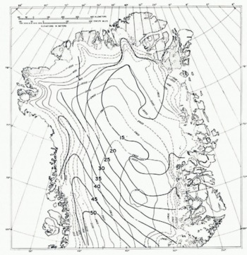
Fig. 2. Isohyetal map of north Greenland. Bold contours in g. cm.−2 of water
Figure 2 also shows the well developed zone of maximum accumulation on the west slope, and its decline with elevation towards the north.
South Greenland
Figure 3 shows isohyets for south Greenland predicted by equation (3). In contrast to north Greenland, a pronounced east-coast accumulation maximum is indicated with a general decrease in accumulation to the west. The high values on the east and south coasts can be attributed to circulation around the semi-permanent Iceland low but the pronounced low accumulation area on the west coast seems somewhat anomalous, particularly when contrasted with the higher accumulation at similar altitudes further north.

Fig. 3. Isolyetal map of south Greenland. Bold contours in g. cm.−2 of water
It should be pointed out that a far larger range of observed accumulation occurs within a smaller area in south Greenland than in north Greenland. In addition warmer temperatures and high accumulation make the possibility of interpretive error in pit studies more likely. The high value of the standard error for Equation (3) reflects the variability of accumulation.
Transition zone
Isohyets for the transition zone are shown in Figure 4. A greater degree of symmetry is shown here than in the regions to the north and south, although there still exists an east-coast maximum. The beginning of the change over to a west-coast maximum is visible. The multiple correlation coefficient R of Equation (4), shows that the model is not as successful as a predictor for this area as for the preceding regions.

Fig. 4. Isohyetal map of transition zone. Bold contours in g. cm.−2 of water
Discussion
Figure 5 shows isohyets for all Greenland (except the Thule peninsula) derived by combining the results of the three separate areas. In combining, isohyets were smoothed and changed somewhat to bring about smooth transitions between regions. The resultant map shows clearly the asymmetric nature of the accumulation pattern. It seems quite evident that this asymmetry is a product of the shape of the ice sheet, of the circulatory pattern existing in this region, and of the distribution of available moisture source areas.

Fig. 5. Isohyetal map of Greenland. Bold contours in g. cm.−2 of water
While the primary purpose here is to delineate the distribution and amounts of mean annual accumulation over the ice sheet, when combined with data for the Thule peninsula (Reference BensonBenson, 1962) it enables a new calculation of the total ice sheet accumulation to be made, which in turn can be used for mass-balance estimates. Inasmuch as the author has serious reservations about the validity of such studies, these calculations and estimates have not been made. For discussions and results of earlier mass-balance studies by traditional methods see Reference LoeweLoewe (1936), Reference BauerBauer (1955), Reference BaderBader (1961), Reference BensonBenson (1962) and Reference BauerBauer (1966). Reference ShumskiyShumskiy (1965) provides a promising alternate method for attacking mass-balance problems on large ice sheets.
Conclusions
Mean annual accumulation at a point can be predicted with a fair degree of accuracy from the parameters latitude, longitude and elevation. Trend surfaces calculated from prediction equations indicate the regional accumulation patterns prevailing on the Greenland ice sheet. The ice sheet shows two major zones of high accumulation; the southern dome, below latitude 67° N. and the west slope of the ice sheet north to latitude 77° N. These zones are ultimately related to cyclonic storm tracks and the presence of moisture source areas along the storm tracks.
Acknowledgements
The author would like to express his appreciation to the members of the Research Division of U.S.A. C.R.R.E.L. for providing many helpful criticisms. SP/4 Roger Doescher capably handled the tedious task of processing the data.


