


Introduction
Changes in environmental conditions in freezing lakes, rivers and reservoirs, induced by climate change and human activities, are ongoing (Reference MagnusonMagnuson and others, 1997; Reference Assel, Cronk and NortonAssel and others, 2003). The annual growth and decay of ice cover are the most visible and predominant phenomena in the surface water bodies, for instance, in northeast and northwest China. Ice thickness is controlled by the local meteorological conditions. Inversely, the intra- and interannual variations of ice thickness influence the local weather and climate (Reference Latifovic and PouliotLatifovic and Pouliot, 2007; Reference Šarauskiená and JurgenlánaitáŠarauskiená and Jurgelánaitá, 2008). One of the most crucial parameters in various ice growth models is the thermal conductivity of ice, which is defined as the transport coefficient of conductive heat flux. Concurrently, the determination of thermal conductivity of ice defines the accuracy of ice thickness models. On the other hand, thermal conductivity of ice controls the exchange potential of heat between the atmosphere and water body, and influences the living environment and ecosystem within and under ice (Reference Stefanovic and StefanStefanovic and Stefan, 2002; Reference Mishra, Cherkauer and BowlingMishra and others, 2011). Thermal properties of ice are also relevant to hydraulic and civil engineering in ice conditions.
A variety of investigations, experimental and theoretical, have been conducted on the thermal conductivities of freshwater ice (Reference Landauer and PlumbLandauer and Plumb, 1956), sea ice (Reference Pringle, Eicken, Trodahl and BackstromPringle and others, 2007) and ground ice (Reference GavrilievGavriliev, 2008). Ice is a temperature-dependent material. Past findings have indicated that the thermal conductivity of pure ice increases with decreasing temperature, ranging from 0°C to –173°C (Reference Landauer and PlumbLandauer and Plumb, 1956; Reference FukusakoFukusako, 1990). At temperatures below –173°C, the thermal conductivity still increases with decreasing temperature, passes through a maximum at about –266°C and then decreases as the temperature decreases further (Reference KlingerKlinger, 1975). However, the conductivity of ice in natural conditions differs from the pure ice case, because it consists of not only ice crystals but also gas inclusions, brine inclusions, solid salt crystals (cold saline ice) and sediments (sand, earth solids and plant debris). Therefore natural ice must be treated as a multi-component, multiphase, porous medium, to which theoretical models can be carefully applied (Reference Shoshany, Prialnik and PodolakShoshany others, 2002; Reference Wang, Pan and ChenWang and others, 2007; Reference Kou, Liu, Wu, Fan, Lu and XuKou and others, 2009). Consequently, the term effective thermal conductivity (ETC) is applied to the reservoir freshwater ice in this paper.
In reservoirs, which do not freeze through the whole water body, only gases and tiny unfrozen brine pockets are usually trapped between ice crystals. However, previous theories have considered only the content of each component in natural ice but not the type, size and shape of ice crystals and gas bubbles. To precisely evaluate the ETC of freshwater ice is the basis of simulations of ice growth and decay and evaluation of the ice/atmosphere transfer processes (Reference SchwerdtfegerSchwerdtfeger, 1963; Reference Pringle, Trodahl and HaskellPringle and others, 2006).
Experimental data show more advantages but are still inadequate. Moreover, most previous work on ice conductivity has been conducted over too wide a temperature range (from 0°C to almost absolute zero). In practice, in nature the range of temperature variation of ice and ambient environment is usually 0 to –25°C, so resolution of the temperature effect of ETC in the available literature does not meet the requirement of numerical simulations of ice thermodynamics in natural freshwater bodies. Furthermore, determining the ETC of ‘warm ice’ (i.e. temperature higher than –5°C) is necessary for ice modeling, since the bottom temperature of floating ice is always at the melting point. However, it is difficult to conduct the experimental tests with warm ice, since an extremely tiny temperature gradient should be built to avoid melting at the interface between the ice and the sensors.
This paper presents the results of a series of laboratory tests for ETC of freshwater ice sampled from a reservoir in northeast China. The tests were performed at temperatures of 0 to –10°C. The internal structure of the ice (e.g. ice crystals and gas bubbles) was observed and introduced to analyze its influence on the ETC. Comparisons were made between the experimental data and the outcome of theoretical models.
Methods and Materials
Sampling sites
In spite of a lack of large lakes, there are many medium-sized and small lakes and reservoirs located in northeast China. Controlled by the cold Siberian winds in winter, freshwater ice covers grow and thaw annually. Ice processes, resulting from the local meteorological conditions, reflect the evolution of the local climate, and change the water-body/atmosphere interaction and the ecological environment of under-ice biota.
Ice samples for the ETC measurements were collected from Hongqipao reservoir, Daqing, Heilongjiang Province. This is a typical large reservoir in Songliao plain, with an area of 35 km2 and a storage of 1.16 × 10⁸m3. The pH of the water in this reservoir is ∼8.25. The concentration of dissolved and suspended substances is approximately 300 ± 2 0 and 22 ± 10 mgL−1, respectively. A great number of grass clusters and fish inhabit Hongqipao reservoir. The water body is static, due to its low or even negligible flow rate. Ice forms and grows thermodynamically under static conditions from early November, and thaws before disappearing in mid- or late April of the following year, so there is a long ice period of 5–6 months. The maximum ice thickness is about 100–110cm. The ice sheet consists mainly of congelation ice, with possibly a thin superimposed ice layer on top (<2cm due to very little snow accumulation and flooding). The ice sheet is mainly granular- (20–35%) and columnar-grained, according to our five-winter observation series from 2008 to 2012. There is no intermediate slush layer in the ice sheet. However, from late March and early April the snow and surface ice start to melt, and liquid water pools appear on the surface. Later, when the ice temperature rises, gas bubbles enlarge by internal melting and inner fissures form, so surface water descends and water content in ice increases. In late April, the ice cover breaks apart.
Equipment and techniques
Generally, techniques for determining the thermal conductivities of solid materials can be divided into steady-state and unsteady-state methods. The quasi-steady-state hot-wire method was adopted in tests using the QTM-D3 thermal conductivity measuring instrument (Japan, Kyoto Electronics) (Fig. 1). In this technique a thin, long wire (often platin or copper wire) is placed along the axis of an infinitely long cylinder with an infinitely long radius, and the hot wire (also acting as a thermistor) is initially in thermal equilibrium with the ambient substance (ice specimen). The wire is then heated with a constant electric current for awhile in order to cause a temperature increment. Since the thermal properties of the hot wire are constant, its rate of temperature increase is controlled by the thermal conductivity of the ambient substance. Conversely, the conductivity of the ambient substance (ice specimen) can be calculated based on the rate of temperature increase.

Fig. 1. The testing instrument: a QTM-D3 thermal conductivity measuring instrument. The hot wire (10 cm long, also acting as a thermistor) fits tightly between the thermal insulator and the ice sample. The data logger also works as a controller which reads the thermal conductivity values and the temperature of the hot wire.
On 26 November 2009 during the fast growth period, an ice block with an intact thickness of 42 cm was sampled. Six cubic ice samples were cut from the ice block along the depth from top to bottom. The surfaces of these samples were smoothed and polished so that the thermo-sensing probe could adhere to the surfaces tightly with no space. Prior to the conductivity measurements, all samples were deposited in a constant-temperature cabinet for ∼12 hours. The horizontal and vertical ETCs of every sample were determined three times, and the mean values were used in the data analysis.
After the thermal conductivity tests, in order to understand the inner structural features of the ice samples, ice crystals and fabrics were investigated and analyzed using the universal stage and PC image-processing programs, based on the techniques formulated by Reference LangwayLangway (1958) and Reference Li, Jia, Huang and LiLi and others (2009).
Results and Discussions
Natural freshwater ice in reservoirs is a compound of pure ice crystal, gas bubble, meltwater in the thawing period, and small amounts of liquid inclusions and sediments. The concentrations, shapes, sizes and arrangements of these elements jointly control the ETC of natural ice. The conductivity of air, water and pure ice is approximately equal to 0.023, 0.54 and 2.22 Wm−1 °C−1, respectively (at –10°C).
Effect of ice crystals and heat transfer directions on ETC
At the initial stage of ice formation, the freezing rate is generally fast (Reference Michel and RamseierMichel and Ramseier, 1971). Granular ice crystals form, owing to a large temperature gradient and strong wind or wave forces. As the ice thickens, the freezing rate slows and individual ice crystals grow downward into larger columnar crystals (Fig. 2). The upper and middle parts of our ice samples (0–32 cm depth) consisted of granular ice, while the bottom part was columnar ice. The equivalent diameters of crystals presented a growing trend with increasing ice thickness (Fig. 3). In addition, ice fabrics revealed that the c-axes of the granular ice layer were randomly distributed in the horizontal plane, while those of the columnar ice layer were oriented in the horizontal plane, suggesting that the granular ice in-plane is isotropic material but the columnar ice in-plane is anisotropic as shown by Reference Michel and RamseierMichel and Ramseier (1971).
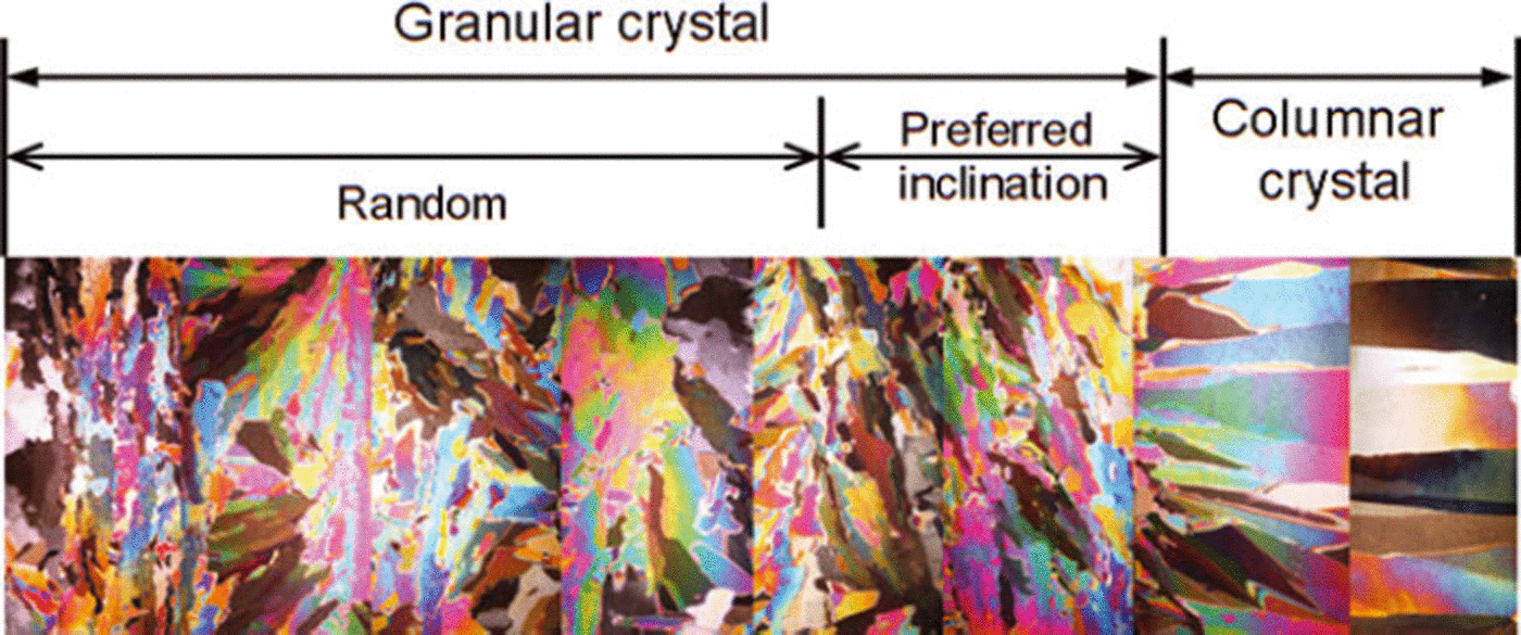
Fig. 2. Vertical sections of freshwater ice crystals.
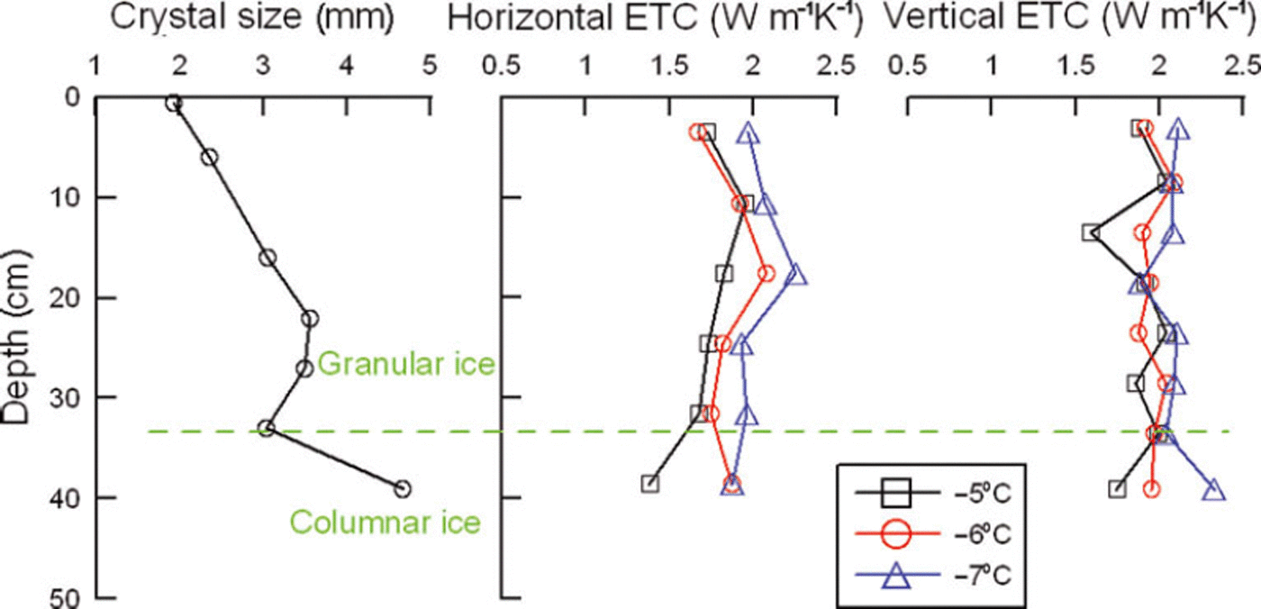
Fig. 3. Profiles of ice crystal size, horizontal and vertical thermal conductivity. Horizontal and vertical thermal conductivity in this paper denotes the conductivity of the direction in which the heat diffuses parallel and perpendicular to the original ice surface, respectively.
The current literature is increasingly focused on vertical thermal conductivity since this plays the key role in heat-conduction and ice growth models. Nevertheless, the horizontal conductivity is also important, in the simulation of local ice temperature field, ice push pressure and thermal expansion force. Figure 3 indicates that as ice crystal sizes increase, the vertical ETC shows no distinct variations. However, the horizontal ETC is slightly weaker than the vertical ETC. It increases first, passes a maximum at ∼20cm depth and then decreases. The ice crystal structure profile in Figure 2 reveals that the crystals have some orientations or regular inclination from 20 cm depth to the bottom of the ice, and besides columnar crystals this layer contains very large granular crystals. Reference Landauer and PlumbLandauer and Plumb (1956) found that the conductivity of monocrystal ice is a little higher (by 5%) parallel to the c-axis than perpendicular to the c-axis, although ETC of artificial and glacier monocrystal ice and polycrystal ice shows few discrepancies. As the ice thickens, the inclinations of ice crystals are more prone to the vertical direction, the heat transmission direction of the hot-wire probe approaches perpendicular to the crystal orientation and the ETC becomes smaller. However, at the same ice temperature, ETCs in different directions are very similar and turn out to have a certain degree of isotropy, because the thermal conductivity of pure ice as a crystalline solid is determined by phonon transfer of thermal energy by a vibrating crystal lattice, almost independent of the macro-structure of the ice crystals (Reference GavrilievGavriliev, 2008).
Effect of gas bubbles and ice densities on ETC
Various shapes of gas inclusions are distributed within natural ice. Figure 4 shows a picture of macro features of gas bubbles in a sample. The 0–12 cm layer contains a mass of tiny gas spheres, making the ice milk-white; the 12–26 cm layer contains a lot of large spherical gas bubbles but much sparser than in the 0–12cm layer; however, only a few bubbles show up from 26 cm depth to the bottom, the layer appearing as clear ice. Therefore, ice sections reveal that the gas content has a declining trend as the ice grows, but ice density shows a distinct reverse trend (Fig. 5), because the gas density is much lower than that of pure ice.

Fig. 4. Photograph of gas bubbles in ice sample (top of the ice is on the left). The bright white portion is gas bubble, and the black portion is pure ice.

Fig. 5. Profiles of ice crystal size, gas bubble size and content, and density against depth. The measured ETC data on the right correspond to a temperature of –7°C.
Freshwater reservoir ice is primarily a two-phase (solid–gas), two-component (pure-ice–gas) compound system, due to the insignificance of brine inclusions as compared with sea ice. In other words, ice samples consist of continuous phase (solid ice crystals, phase I) and stochastic discontinuous phase (gas bubbles, phase II). Reference Hamilton and CrosserHamilton and Crosser (1962) proposed an ETC equation for this system:

where K and V denote the ETC and volumetric content, subscripts 1 and 2 denote phases I and II, respectively, and n is an experimental constant influenced by the shape of dispersing granules (i.e. phase II) and the conductivity ratio of the two phases. For spherical dispersing granules, n=3. Figure 4 indicates that all the gas bubbles in the sample are spherical or quasi-spherical, so the ETC can be calculated by

The thermal conductivity of pure ice and air (at –10°C) is regarded as 2.22 and 0 W m−1 °C−1 approximately, separately, and can be taken into Eqn (2) to obtain the ETC of natural freshwater:

Thus, the theoretical values of ETC can be obtained (Fig. 5) when the gas contents of the samples are substituted into Eqn (3).
It is clear that the calculated ETC matches very well the experimental ETCs for natural freshwater ice in the present study. As the ice thickness increases, the content and size of gas bubbles decrease rapidly, and then reach and maintain a certain level. The ETC shows an indistinct increasing trend against ice depth. Minor effects of gas content and ice density on the ETC were detected in this research, predominantly because the gas content (0–3%) and the variations of gas content and ice density were too small to have visible impacts on the ETC.
Effect of temperature on ETC
Natural ice is a sensitive temperature-dependent material so that nearly all of the properties of ice are controlled and influenced by the ice temperature (Reference Light, Maykut and GrenfellLight and others, 2003). A large number of previous investigations have been conducted to evaluate the effects of temperature on the thermal conductivity, and many empirical and theoretical equations have been formulated.
The thermal conductivity of pure ice is four times as large as that of pure water and is higher than that of air by about two orders of magnitude. In the very beginning of congelation ice formation, with temperature of 0 to –4°C, phase transitions (water freezes into ice crystal) take place and ice crystals appear and conglomerate rapidly to shape a stable state. However, the ETC of the evolving system will rise rapidly in the temperature range between the melting point and stable-state point rather than change abruptly at the melting point. When ice temperature is depressed lower than –5°C, the ETC will stabilize basically (Reference Li, Meng, Yan, Jin and YuLi and others, 1992) or increase very slowly (Reference Chen, Morikawa, Kishi and HashimotoChen and others, 2005, for thermal diffusivity).
When the ice temperature is very low and changes in a wide range (e.g. 0–173°C), Reference Sakazume and SekiSakazume and Seki’s (1978) formula is recommended by Reference FukusakoFukusako (1990) to determine the conductivity of pure ice:

where K, θ and subscript i denote thermal conductivity, ice temperature and ice, respectively. However, Eqn (4) cannot be applied at high ice temperature; it covers a large temperature range and does not describe accurately the variation of ETC in detail at the melting point. Also the formula is for pure ice, which is not representative of the ice in natural waters. Furthermore, the thermal properties at high temperature (especially 0 to –10°C) would be critical for understanding and computing ice fracture, ice push and ice-cover decay in natural waters.
The ETCs of reservoir ice measured in the laboratory are compiled in Figure 6 at high temperatures of 0 to –10°C. It is evident that the ETCs of ice samples in both directions decrease nonlinearly, when the ice temperature rises from –10°C to 0°C. ETC increases rapidly from 0°C to lower temperatures, reaches 2.25Wm−1K−1 at about –5°C, and then changes very little. Given that ETC discrepancies were tiny in different directions and at different depths and can be neglected in this paper, we compiled all data together in Figure 7 for comparison with previous results.

Fig. 6. Relationship between horizontal (a) and vertical (b) ETC and temperature.

Fig. 7. ETC of reservoir ice as a function of temperature. The circles denote the measured data, and the green, pink and blue lines are proposed by Reference Sakazume and SekiSakazume and Seki (1978; pure ice), Reference Li, Meng, Yan, Jin and YuLi and others (1992; sea ice near an estuary) and Reference SchwerdtfegerSchwerdtfeger’s (1963) model (sea ice of ∼0.3 ppt salinity), respectively. The dotted line is proposed for estimating ETC of natural reservoir ice based on present tests. The circles and vertical bars in the lower part refer to mean values and standard deviations of ETC within a 2°C interval against the corresponding averaged temperature.
Note that the present conductivity values are between those from Reference Sakazume and SekiSakazume and Seki (1978) (pure ice) and Reference Li, Meng, Yan, Jin and YuLi and others (1992) (sea ice of 4 ppt salinity). The plausible reason is that there could be some liquid pockets within this reservoir ice due to the dissolved matter in the parent water (∼300 mg L−1). This is probably also why the present conductivity-temperature has a similar shape to that in Reference Li, Meng, Yan, Jin and YuLi and others (1992) (the conductivity decreases rapidly with ice temperature close to melting point). An approximate curve (applying Reference SchwerdtfegerSchwerdtfeger’s (1963) and Reference Pringle, Trodahl and HaskellPringle and others’ (2007) sea-ice equations) is proposed to estimate the ETC at high temperature of the reservoir ice. Note that this curve matches well with the present results at temperature below –4°C, while a strong discrepancy exists above –4°C despite their similar tendency.
Some intrinsic deficiencies in the apparatus used may account for this. On the one hand, the minor temperature increment A T (uncontrollable in this study) induced by the heating of hot wire is not taken into consideration for the representative temperature T r, which should be equal to T+ΔT/2 instead of T (T is the ice temperature before the measurement). On the other hand, the closer to the melting point the ice temperature is, the smaller is the temperature increment required to avoid ice melting. This calls for much more accurate temperature measurement, which may be beyond the capability of the instrument used here. The reasons mentioned above largely account for the gap between this curve and the calculated curve of Reference SchwerdtfegerSchwerdtfeger’s (1963) ‘bubbly sea ice’ model. Another reason may lie in the complicated effect of gas bubble structure on the ETC of ice (Reference Wang, Carson and NorthMFand ClelandWang and others, 2008).
Generally determining the thermal conductivity of ice at a temperature close to the melting point requires much more careful measurement techniques and accuracy. When the spring melting season arrives, reservoir ice temperature increases, the walls of gas voids melt and liquid water inclusions form, resulting in a broadening and merging of gas pockets to form gas tubes (Reference Light, Maykut and GrenfellLight and others, 2003, Reference Light, Maykut and Grenfell2004). Furthermore, the high temperature weakens the intercrystal bonds, and intercrystal fractures appear, expand and link up, forming more tubes. All of these secondary pockets and tubes, saturated or unsaturated with surface and interior meltwater (Reference Golden, Ackley and LytleGolden and others, 1998; Reference GoldenGolden, 2001), markedly increase the contents of gas and water, and this decaying process should be properly understood to determine the conductivity of natural ice, including lake and reservoir ice with tiny impurities.
Conclusions
The ETC of natural fresh water was examined for its dependency on temperature and impurities in the ice. Ice samples were collected from a typical reservoir in northeast China. The concentration of dissolved substances in the reservoir water was ∼300mgL−1. The ice samples were tested in the laboratory to determine the ETC, with attention to high temperature of 0 to –10°C. A comparative study of ETC was conducted between the present measurements and existing semi-empirical formulae. The findings were as follows:
-
1. The reservoir freshwater ice grows thermodynamically in a static and calm state. Ice section analysis indicated that the entire ice samples were mostly granular ice, besides a 10cm bottom layer of columnar ice. Vertical ETC showed differences with ice crystal type and size, while horizontal ETC had a regular relation with crystal type and size, predominantly impacted by the intersection angle between the heat flux and ice crystal.
-
2. The gas bubbles trapped in ice sample were spherical or quasi-spherical. Theoretical and measured ETC data were in good agreement and demonstrated jointly that the gas content (<3%) and the size of the gas bubbles were too small to have a significant influence on the ETC of the reservoir ice.
-
3. At high temperature of 0 to –10°C, the ETC experienced a complicated evolution due to a minor fraction of unfrozen water and other impurities, with resemblance to sea ice. When the ice temperature rose above ∼–4°C, the ETC decreased much more rapidly than at lower temperatures, especially those below about –10°C. A coarse curve applying Reference SchwerdtfegerSchwerdtfeger’s (1963) and Reference Pringle, Trodahl and HaskellPringle and others’ (2007) models for sea ice was fitted based on the present analysis, and is recommended to evaluate the natural reservoir ice (see Fig. 7). However, the measured thermal conductivities for temperatures higher than –4°C were less than expected from previous work on saline ice. Whether this was due to the measurement techniques or actual properties of the reservoir ice is not clear.
Determining the thermal conductivity of ice in natural water bodies at a temperature close to its melting point is a difficult task. Much more careful work is required, in terms of measurement techniques, accuracy, the processes involved, and in understanding the evolution of the internal structure of the ice. Given the importance of thermal conductivity in modeling ice growth and decay and understanding thermal stresses, much more effort needs to be devoted to this question in future work.
Acknowledgements
This work was continuously supported by the National Natural Science Foundation of China (No. 51079021, No. 51221961) and the Open Fund of the State Key Laboratory of Frozen Soils Engineering (No. SKLFSE200904, No. SKLFSE201202), Cold and Arid Regions Environmental and Engineering Research Institute, Chinese Academy of Sciences. We examined the gas effect on ice thermal conductivity with the support of the Vilho, Yrjö and Kalle Väisälä fund of the Finnish Academy of Sciences and Letters. We thank the staff at Hongqipao reservoir who helped us with the field program. We also thank two anonymous reviewers and Matti Leppäranta for constructive comments and advice on improving the paper.


