


Impact Statement
Microstructured, or nanostructured surfaces provide significant advantages and functionalities for industrial applications requiring (i) improved wettability (self-cleaning surfaces, fluid transport, microfluidic systems), (ii) enhanced adhesion (new adhesives), (iii) reduced friction and wear (efficiency and optimized lifetime and of mechanical parts), (iv) specific optics (antireflective coatings, optical filters, high-yield solar cells), (v) controlled cell growth (tissue engineering and regenerative medicine), (vi) improved antimicrobial properties (physical disruption of bacteria) or (vii) drag reduction.
Currently, the mass production of these surfaces uses processes such as ion or chemical etching, sol-gel processing, templated hot embossing, laser texturing, colloidal lithography, Langmuir–Blodgett films (LB), etc. Unfortunately, all these methods are limited (i) in flexibility (pattern geometry, periodicity tuning, materials choice), (ii) in productivity due to multistep processing and (iii) in scalability to large surfaces and roll-to-roll processes.
The proposed innovative true roll-to-roll LB type technique for surface texturing could overcome all the above limitations.
1. A high-performance LB type process: objectives, description and benefits
The LB technique is a widely known method for assembling on a liquid interface and depositing onto a solid substrate a compact monolayer of nanoparticles as a thin film (Reference PettyPetty 1996; Reference Bardosova, Pemble, Povey and TredgoldBardosova et al. 2010). This process allows the building of controlled nanoscale architectures for a variety of applications in material sciences, nanoelectronics, photonics, energy (Reference Fang, Yoon, Hubble, Tran, Kostecki and LiuFang et al. 2022) and biosensors (see, e.g. Reference Cai, Li, Ravaine, He, Song, Yin, Zheng, Teng and ZhangCai et al. 2021). In the conventional LB process (Reference BlodgettBlodgett 1938), nanoparticles dispersed in a volatile solvent are spread on a subphase surface and compressed with a moving motorized barrier, gradually reducing the free space between particles to form a compact monolayer (figure 1a,b). The substrate is then withdrawn vertically from the liquid. The nanoparticle monolayer is transferred onto the substrate by carefully controlling the withdrawal speed. At the same time, the barrier follows the motion to keep a constant push on the particles floating on the liquid film surface. This sequence can be repeated several times to obtain multilayer structures with precise control of packing density.

Figure 1. Comparison of the original LB process (a, b) with the present roll-to-roll LB-type process (c, d) with a flowing subphase. (a) Particles are spread over the air–subphase interface between a moving barrier and a partially immersed vertical substrate. (b) The moving barrier pushes the particles and when the nanoparticles form a target lattice, the substrate is withdrawn at the same speed as the barrier's speed and collects the particle lattice. (c) The liquid subphase flows in a laminar regime down a ramp and continuously conveys particles on its upper part, a roller-driven film is partially immersed in this subphase. (d) The accumulation of particles at the liquid surface and the compression due to the subphase movement lead to a compact monolayer continuously transferred onto the rotating roller.
For monodispersed spherical particles with diameters in the range of 300–2000 nm, the monolayer can exhibit structural colours (Reference Delléa, Shavdina, Fugier, Coronel, Ollier, Désage and RatchevDelléa et al. 2014) arising from the interference and diffraction of light due to the hexagonal close-packed (HCP) structure (figure 2).

Figure 2. (a) Microscopic view of HCP structure of silica spheres (diameter 1.1 μm) obtained by LB-type process on a diamond-like carbon substrate. (b,c) Macroscopic view of structural colours on a diamond-like carbon substrate (5 × 5 cm2).
One of the major advantages of the LB process is the ability to create well-ordered, two-dimensional (2-D) arrays of nanoparticles with precise control over their size, shape and spacing. It allows the creation of unique optical and electronic properties that are not achievable with bulk materials. The LB process has been used to create and develop various new nanoparticle-based devices, including biosensors, batteries, photovoltaic cells and electronic devices (Reference Oliveira, Caseli and ArigaOliveira, Caseli & Ariga 2022).
While the original LB method was developed for small-area applications, the technique has been scaled up to enable the fabrication of large-area thin films; however, addressing large surfaces with LB is technically challenging to maintain a high level of uniformity across the entire surface. If the LB film is not uniform, performances in certain applications can be irregular, depending on the surface area considered. Some applications require rigorous homogeneous large-scale LB films, (i) to enhance photon absorption in photovoltaic solar cells (Reference Grenet, Emieux, Delléa, Gerthoffer, Lorin, Roux and PerraudGrenet et al. 2017) or (ii) to reduce friction between machine moving parts.
The roll-to-roll process was the first approach for scaling up the LB process (Reference Parchine, McGrath, Bardosova and PembleParchine et al. 2016): a roller is partially immersed into the static subphase, and a flexible substrate is continuously fed through it. The principle is quite similar to standard LB, but the roller stops at the end of the film transfer, and the barrier is moved back to restart the deposition process at step. This roll-to-roll LB process allows deposit on a large surface. Still, it is, in fact, sequential, considering the necessity to restart the sequence with a barrier at its initial position.
The barrier is thus a limiting factor towards large surface fabrication and productivity. To overcome this limitation, our approach, inspired by Reference Schneider and PicardSchneider & Picard (2008), involves replacing the barrier with a horizontal feed zone and an inclined ramp partially immersed over which the liquid subphase trickles down with an imposed low flow rate to ensure a laminar regime (figure 1c). The liquid is fed through a tube pierced with small holes and lying on the horizontal feed zone.
When particles start being deposited on the liquid film surface at the top of the ramp or upstream in the horizontal feed zone (figure 3a), they follow down the current and start accumulating on the film surface in the transfer zone, then in the lower part of the ramp and finally just upstream of the first hydraulic jump (figures 1d and 3a). The rotational speed of the roller controls the withdrawal velocity of a flexible substrate coated with a compact hexagonal array of particles. This design allows the continuous manufacturing of HCP particle arrays on a flexible substrate of large dimensions.

Figure 3. (a) The LB with dynamic liquid flowing down a ramp (particles and film thickness are not to scale). (b) Quasi-top-view of the second hydraulic jump and the iridescence induced by the compact film of particles.
The particle-coated film free surface is generally visible to the naked eye because of diffusion or interference phenomena with white light-emitting-diode light (figure 3b).
Our LB-type design involving a liquid flowing down a ramp presents several advantages in comparison with standard LB technique: (i) scalability – roll-to-roll processing allows deposition on very long, flexible surfaces like rolls of plastic, metal, or paper; (ii) continuous processing – monolayers can be deposited continuously at high speeds instead of batchwise on individual substrates; (iii) large area uniformity – uniform monolayers can potentially be deposited over very large areas on rolls; (iv) improved efficiency – continuous processing and larger volumes could make the manufacture of monolayer cost-effective compared with batchwise standard LB.
More generally, our design based on a dynamic liquid subphase could offer significant additional capabilities compared with the standard LB barrier-based systems used for nanoparticle deposition. For example, it could allow the nanoparticles to be arranged in a uniform optimized array and different surface pressures to be targeted. This paper focuses primarily on fine particles (280–1100 nm) arranged in HCP arrays. The case of nanoparticles with targeted surface pressures is currently outside the scope of our work.
From the hydrodynamic point of view, successive flow patterns downstream from the feed can be observed.
i. A laminar Nusselt inclined liquid film (smooth for low flow rate, wavy for higher flow rate due to the pump fluctuations), whose thickness is investigated in § 2.1,
ii. A first hydraulic jump (figure 3) resulting from the interaction between the free surface flow and the particle coated surface flow with zero tangent velocity. Its profile is examined experimentally in § 4 and with numerical modelling in § 5,
iii. A particle-covered inclined liquid film, whose thickness is explored in § 2.2. The particle bed properties is characterized in § 6.2,
iv. A second hydraulic jump (figure 3), which is not studied in the present work,
v. A particle-covered horizontal liquid film, characterized in § 6.3.
The dynamic liquid subphase gives rise to peculiar hydraulic phenomena, which can be essential for nanoparticle assembly. Understanding the hydraulic aspects is crucial for the possibilities of innovation and expansion of the technique.
In this work, we investigate for the first time the hydraulic behaviour of an LB-type process with dynamic liquid with four optical techniques to qualify and characterize the influence of the film flow rate on the particle assembly. The first two methods are complementary to get information on the film thickness and hydraulic jump profile: (i) the confocal film thickness technique provides accurate information on absolute thickness and first jump profile without precise location on the longitudinal position (§ 3), whereas (ii) the fringe projection/moiré technique allows resolving the longitudinal evolution of the interface elevation (§ 4). Only a numerical model (§ 5) makes it possible to obtain the longitudinal evolution of the film thickness, with additional insights into the fluid velocity field. The two other optical techniques give information on (iii) the particle centre-to-centre distances with a Bragg diffraction technique (§ 6.2) and (iv) the size of the single crystal zones with a colour technique (§ 6.3).
All measurements presented in the following sections were performed with no withdrawal. The withdrawal speed is an additional parameter that would entail a more comprehensive study. However, it is unnecessary regarding process control since the best particle-coated-film buildup is always obtained with low withdrawal.
2. The system hydrodynamic model
Let us consider a thin liquid film trickling down a smooth plate inclined at an angle  $\alpha \ne 0$ to the horizontal with an imposed flow rate (figure 4). Downstream from the feed, there is no shear stress on the free surface, a flow pattern that we will call the Nusselt regime. Farther downstream, the surface of the liquid film is covered by a densely packed monolayer of nanoparticles or by a flexible ultrathin membrane made up of a soft material. The film thickness then adapts itself to this new situation. This configuration imposes a zero velocity on the top liquid surface, a flow pattern that we will call the Poiseuille regime.

Figure 4. Liquid film flowing downward on an inclined plate in the Nusselt and Poiseuille regimes: Nusselt regime, zero shear stress at the free surface (thin line); Poiseuille regime, zero velocity at the upper surface (thick line).
The analysis of the time-independent base flow developed in the following aims to determine the dominant physical phenomena and predict the film thickness change along the plate. The conditions and assumptions will be specified in due course.
First, we will investigate the consequences of two conditions, i.e. having a thin film and a low Reynolds number. Then, we will obtain each regime's dimensional and dimensionless governing equations to be solved to get the change in the liquid film thickness along the plate.
2.1 The Nusselt regime
First, we will recall some results on the flow of a film of constant thickness along the plate. Second, we will study the wavy flow of a thin film.
2.1.1 The film of constant thickness
Assuming that the liquid film thickness does not change along the plate, its value can be obtained from the Nusselt–Jeffreys equation
 \begin{equation}{h_N} = {\left( {\frac{{3\mu Q/W}}{{\rho g\,\textrm{sin}\,\alpha }}} \right)^{1/3}}.\end{equation}
The above equation involves four quantities of interest: the thickness  ${h_N}$; the dynamic viscosity $\mu $; the volume flow rate per unit width of the film $Q/W$; the gravity force per unit volume $\rho g\,\textrm{sin}\,\alpha $. The dimensions of these quantities can be expressed in terms of three base dimensions, i.e. length, pressure and time. As a result, (2.1) reduces to a single dimensionless group called the Jeffreys number Je, which is a constant in this film region,
 \begin{equation}J{e_N}\,\,\hat{ = }\,\,\frac{{h_N^3\rho g\,\textrm{sin}\,\alpha }}{{\mu Q/W}} = 3.\end{equation}
The Jeffreys number, first introduced by Reference O'KeefeO'Keefe (1969), can be interpreted as the ratio of the scale of potential (gravitational) energy to the scale of energy dissipated by viscous friction.
As we are particularly interested in the change in the film thickness in terms of the flow rate, we may define a Reynolds number  $Re$ as follows:
 \begin{equation}Re\,\,\hat{ = }\,\,\frac{{Q/W}}{\nu },\end{equation}
where  $\nu $ is the kinematic viscosity.
2.1.2 The wavy flow of a thin film
Figure 4(a) represents the flow under consideration. Let the length of the plate L and  ${h_0}$ be the scales of x and y, respectively.
The main assumptions of our model are the following:
i. the flow is steady and 2-D in the $x$- and $y$-directions;
ii. the film is thin,
$\varepsilon \,\hat{ = }\, {h_0}/L \ll 1$, which implies that its free surface is gently sloped since
(2.4)\begin{equation}\frac{{\textrm{d}h(x)}}{{\textrm{d}x}} \sim {h_0}/L \ll 1;\end{equation}iii. the Reynolds number defined by (2.3) is small, typically
$Re < 50$.


Only retaining the terms of order 0 in  $\varepsilon $, the $x$- and $y$-momentum equations, read, respectively,
 \begin{equation}0 = {-} \frac{1}{\rho }\frac{{\textrm{d}p}}{{\textrm{d}x}} + \nu \frac{{{\textrm{d}^2}u}}{{\textrm{d}{y^2}}} + g\,\textrm{sin}\,\alpha ,\end{equation}
 \begin{equation}- \frac{1}{\rho }\frac{{\textrm{d}p}}{{\textrm{d}y}} - g\,\textrm{cos}\,\alpha = 0.\end{equation}
As the liquid film is wavy, we have to the surface tension  $\sigma $ and consider the momentum balance at the free surface, which we will simplify by using the following assumptions:
i. there is no phase change at the free surface;
ii. the gas phase intervenes only by its pressure
${p_G}$ assumed constant;iii. the surface tension
$\sigma $ is constant.


In that case, the momentum balance at the interface reduces to
 \begin{equation}p[y = h(x)] = {p_G} - \sigma \frac{{{\textrm{d}^2}h}}{{\textrm{d}{x^2}}},\end{equation}
where  $- {\textrm{d}^2}h/\textrm{d}{x^2}$ is the curvature of the free surface for a nearly unidirectional flow.
Integrating the  $y$-momentum balance (2.6) from an arbitrary y to the film surface $y = h(x)$ and accounting for (2.7), we obtain the pressure field in the liquid film,
 \begin{equation}p(x,y) = {p_G} + \rho g\,\textrm{cos}\,\alpha (h - y) - \sigma \frac{{{\textrm{d}^2}h}}{{\textrm{d}{x^2}}}.\end{equation}
An important consequence is that  $\textrm{d}p/\textrm{d}x$ does not depend on y since
 \begin{equation}\frac{{\textrm{d}p}}{{\textrm{d}x}} = \rho g\,\textrm{cos}\,\alpha \frac{{\textrm{d}h}}{{\textrm{d}x}} - \sigma \frac{{{\textrm{d}^3}h}}{{\textrm{d}{x^3}}}.\end{equation}
To obtain the liquid velocity profile  $u(x,y)$, we integrate the $x$-momentum (2.5) with the following two boundary conditions. The first is a no-slip condition at the wall:
 \begin{equation}u(x,0) \equiv 0\quad \textrm{for}\ \textrm{any}\ x.\end{equation}
The second is a zero shear stress at the free surface. As the flow is nearly unidirectional in x, it reads
 \begin{equation}{\left. {\frac{{\textrm{d}u}}{{\textrm{d}y}}} \right|_{y = h(x)}} \equiv 0\quad \textrm{for}\ \textrm{any}\ x.\end{equation}
Integrating (2.5) and using the two boundary conditions yields
 \begin{equation}u(x,y) = \left( { - \frac{{\textrm{d}p}}{{\textrm{d}x}} + \rho g\,\textrm{sin}\,\alpha } \right)\frac{1}{{2\mu }}y(2h - y).\end{equation}
The liquid mass flow rate per unit width of the film  $Q/W$ is given and can be calculated by integrating the liquid velocity profile (2.12):
 \begin{equation}Q/W\,\hat{ = }\,\int_0^{h(x)} {u(x,y)\,\textrm{d}y} = \left( { - \frac{{\textrm{d}p}}{{\textrm{d}x}} + \rho g\,\textrm{sin}\,\alpha } \right)\frac{1}{{3\mu }}{h^3}(x).\end{equation}
Calculating the pressure gradient in (2.13) from (2.8) we obtain
 \begin{equation}Q/W = \frac{\rho }{{3\mu }}{h^3}\left( {g\,\textrm{sin}\,\alpha - g\,\textrm{cos}\,\alpha \frac{{\textrm{d}h}}{{\textrm{d}x}} + \frac{\sigma }{\rho }\frac{{{\textrm{d}^3}h}}{{\textrm{d}{x^3}}}} \right).\end{equation}
This equation is an integrated form equivalent to the one proposed by Reference PozrikidisPozrikidis (2009) (equation (9.2.11), p. 508). Introducing the Nusselt thickness (2.1), we get the liquid thickness evolution dimensional equation along the  $x$-axis:
 \begin{equation}h_N^3 = {h^3}\left( {1 - \frac{1}{{\textrm{tan}\,\alpha }}\frac{{\textrm{d}h}}{{\textrm{d}x}} + \frac{\sigma }{{\rho g\,\textrm{sin}\,\alpha }}\frac{{{\textrm{d}^3}h}}{{\textrm{d}{x^3}}}} \right).\end{equation}
For a film of constant thickness, we retrieve  $h = \ {h_N}$.
A dimensional analysis allows the dimensional equation (2.15) to be transformed into a dimensionless equation by defining the following dimensionless groups:
 \begin{equation}X\,\hat{ = }\,\frac{x}{{{L_{cap}}}},\quad H\,\hat{ = }\,\frac{h}{{{L_{cap}}\,\textrm{tan}\,\alpha }},\quad {H_N}\,\hat{ = }\,\frac{{{h_N}}}{{{L_{cap}}\,\textrm{tan}\,\alpha }},\end{equation}
where  ${L_{cap}}$ is the Laplace capillary length defined by
 \begin{equation}{L_{cap}}\,\hat{ = }\,\sqrt {\frac{\sigma }{{\rho g\,\textrm{cos}\,\alpha }}} .\end{equation}
The dimensionless grouping  ${H_N}$ has a simple physical significance since we can write
 \begin{equation}{H_N} = \frac{{\rho g{h_N}\,\textrm{cos}\,\alpha }}{{\rho g{L_{cap}}\,\textrm{sin}\,\alpha }},\end{equation}
which is the ratio of the  $y$-hydrostatic pressure change along ${h_N}$ to the $x$-hydrostatic pressure change along ${L_{cap}}$.
Using these dimensionless variables in the dimensional equation (2.15) gives the dimensionless liquid thickness evolution equation along the  $x$-axis
 \begin{equation}H_N^3 = {H^3}\left( {1 - \frac{{\textrm{d}H}}{{\textrm{d}X}} + \frac{{{\textrm{d}^3}H}}{{\textrm{d}{X^3}}}} \right).\end{equation}
Equation (2.19) shows that the solution  $H(X)$ depends on a single dimensionless group, namely, ${H_N}$.
For practical reasons, we can singularize the imposed volume flow rate  $Q/W$ per unit width by using the Reynolds number $Re$ (2.1) and defining a Morton number by
 \begin{equation}Mo\,\hat{ = }\,\frac{{{\rho ^3}g{\nu ^4}}}{{{\sigma ^3}}},\end{equation}
which depends only on the physical properties of the fluid and the gravity constant. Equation (2.19) now reads
 \begin{equation}3M{o^{1/2}} \frac{{{{(\textrm{cos}\,\alpha )}^{1/2}}}}{{{{(\textrm{tan}\,\alpha )}^4}}}Re = {H^3}\left( {1 - \frac{{\textrm{d}H}}{{\textrm{d}X}} + \frac{{{\textrm{d}^3}H}}{{\textrm{d}{X^3}}}} \right).\end{equation}
For convenience, we will define a dimensionless system parameter  $\varSigma $ by
 \begin{equation}\varSigma \,\hat{ = }\, M{o^{1/2}} \frac{{{{(\textrm{cos}\,\alpha )}^{1/2}}}}{{{{(\textrm{tan}\,\alpha )}^4}}} \end{equation}
and get
 \begin{equation}3\varSigma Re = {H^3}\left( {1 - \frac{{\textrm{d}H}}{{\textrm{d}X}} + \frac{{{\textrm{d}^3}H}}{{\textrm{d}{X^3}}}} \right).\end{equation}
The interest of this formulation is to be able to determine, for a given value of the system parameter  $\varSigma $, the profile of the liquid film $H(X)$ for different values of the Reynolds number $Re$.
$Re$.
2.2 The Poiseuille regime
2.2.1 The wavy flow of a thin film
For a gravity-driven Poiseuille flow, the thickness  ${h_P}$ is given by
 \begin{equation}{h_P} = {\left( {\frac{{12\mu Q/W}}{{\rho g\,\textrm{sin}\,\alpha }}} \right)^{1/3}}.\end{equation}
The above equation is the same as the Nusselt–Jeffreys equation (2.1), where the coefficient 3 is replaced by 12. Consequently, the dimensionless groups are the same, and the dimensionless equation reads
 \begin{equation}J{e_P}\,\hat{ = }\,\frac{{h_P^3\rho g\,\textrm{sin}\,\alpha }}{{\mu Q/W}} = 12.\end{equation}
2.2.2 The film of constant thickness
We will follow the same steps as in the analysis of the Nusselt regime. The momentum balance at the upper surface is identical to that used for the Nusselt regime:
 \begin{equation}p[y = h(x)] = {p_G} - \sigma \frac{{{\textrm{d}^2}h}}{{\textrm{d}{x^2}}}.\end{equation}
However, the surface tension is now that of a film surface covered by a densely packed monolayer of nanoparticles. To a first and crude approximation, we will take the same value as in the Nusselt regime film flow. It will always be possible to investigate the sensitivity of the final results to the surface tension. This has not been done in the present paper.
The pressure field in the liquid film is given by the same (2.8) as in the Nusselt regime:
 \begin{equation}p(x,y) = {p_G} + \rho g\,\textrm{cos}\,\alpha (h - y) - \sigma \frac{{{\textrm{d}^2}h}}{{\textrm{d}{x^2}}}.\end{equation}
Integrating the  $x$-momentum equation (2.7) requires two boundary conditions. The first one is a no-slip condition at the wall:
 \begin{equation}u(x,0) \equiv 0\quad \textrm{for}\ \textrm{any}\ x.\end{equation}
The second one is a no-slip condition at the surface of the film:
 \begin{equation}u[x,h(x)] \equiv 0\quad \textrm{for}\ \textrm{any}\ x.\end{equation}
The integration provides a new velocity profile, different from that found in the Nusselt regime:
 \begin{equation}u(x,y) = \left( { - \frac{{\textrm{d}p}}{{\textrm{d}x}} + \rho g\,\textrm{sin}\,\alpha } \right)\frac{1}{{2\mu }}y(h - y).\end{equation}
Integrating the new velocity profile (2.30) yields the imposed volume flow rate per unit width of the film:
 \begin{equation}Q/W\,\hat{ = }\,\int_0^{h(x)} {u(x,y)\,\textrm{d}y} = \left( { - \frac{{\textrm{d}p}}{{\textrm{d}x}} + \rho g\,\textrm{sin}\,\alpha } \right)\frac{1}{{12\mu }}{h^3}(x).\end{equation}
The only difference with the Nusselt regime (2.13) is the new coefficient 1/12 instead of 1/3.
Calculating the pressure gradient in (2.31) from (2.27), we obtain the dimensional film thickness evolution equation for the Poiseuille regime:
 \begin{equation}h_P^3 = {h^3}\left( {1 - \frac{1}{{\textrm{tan}\,\alpha }}\frac{{\textrm{d}h}}{{\textrm{d}x}} + \frac{\sigma }{{\rho g\,\textrm{sin}\,\alpha }}\frac{{{\textrm{d}^3}h}}{{\textrm{d}{x^3}}}} \right).\end{equation}
The only difference with the Nusselt regime (2.15) is that  ${h_N}$ is replaced by ${h_P}$ on the left-hand side.
By defining similar dimensionless quantities as in the Nusselt regime,
 \begin{equation}X\,\hat{ = }\,\frac{x}{{{L_{cap}}}},\quad H\,\hat{ = }\,\frac{h}{{{L_{cap}}\,\textrm{tan}\,\alpha }},\quad {H_P}\,\hat{ = }\,\frac{{{h_P}}}{{{L_{cap}}\,\textrm{tan}\,\alpha }},\end{equation}
we finally get the dimensionless film equation in the Poiseuille regime:
 \begin{equation}H_P^3 = {H^3}\left( {1 - \frac{{\textrm{d}H}}{{\textrm{d}X}} + \frac{{{\textrm{d}^3}H}}{{\textrm{d}{X^3}}}} \right).\end{equation}
Equation (2.34) shows that the solution  $H(x)$ depends on a single dimensionless group, namely, ${H_P}$; as we have
 \begin{equation}H_P^3 \equiv 4H_N^3\end{equation}
the dimensionless film equation in the Poiseuille regime can also be rewritten as
 \begin{equation}4H_N^3 = {H^3}\left( {1 - \frac{{\textrm{d}H}}{{\textrm{d}X}} + \frac{{{\textrm{d}^3}H}}{{\textrm{d}{X^3}}}} \right).\end{equation}
Or, in terms of the system parameter  $\varSigma $ and the Reynolds number Re,
 \begin{equation}12\varSigma Re = {H^3}\left( {1 - \frac{{\textrm{d}H}}{{\textrm{d}X}} + \frac{{{\textrm{d}^3}H}}{{\textrm{d}{X^3}}}} \right).\end{equation}
3. The liquid film thickness at a given point of the ramp
The liquid flows down the ramp and reaches a fully developed velocity profile and a constant thickness  ${h_N}$ (2.1) resulting from the equilibrium between the change in potential energy and the energy due to viscous dissipation. When the liquid encounters the HCP film floating at the subphase-air interface, the velocity profile adapts to the top boundary condition, i.e. a quasizero tangent velocity resulting from the particles jamming, which induces a hydraulic jump. Downstream of the first hydraulic jump, the solid wall on the bottom and the particle bed on the top limit the viscous flow. In this region, the Poiseuille regime is a good estimate ( ${h_P}$, 2.24). The formation and stationarity of the hydraulic jump result mainly from the particles cluttering up and the resulting quasizero tangent velocity.
It is possible that the tangential velocity of the top surface is not strictly zero since several nanoscopic forces (van der Waals, electrostatic), forces associated with particle rotations and capillary forces may have some effects. The confocal chromatic sensing technique will be used to evaluate the quality of the no-slip condition under the particle bed (§ 3.1). Actually, experimental data reported in § 3.2 will not exclude a slight liquid shift under the particle cover. Nonetheless, it is so small that a zero velocity and a Poiseuille velocity profile are sufficient to describe the film behaviour in this region.
In the following section, we first investigate the thickness of the liquid film flowing down the ramp using the confocal chromatic sensing technique. Experiments were performed first with 280 nm SiO2 particles, second with 1100 nm particles and third with a continuous, flexible, thin plastic film (Parafilm). Other diameters of particles were tested but not reported here, which showed similar and consistent results.
3.1 The confocal chromatic technique
Relying on the chromatic aberrations, the confocal sensing technique (e.g. Reference Lel, Al-Sibai, Leefken and RenzLel et al. 2005; Reference Zhou, Gambaryan-Roisman and StephanZhou, Gambaryan-Roisman & Stephan 2009; Reference Berto, Lavieille, Azzolin, Bortolin, Miscevic and Del ColBerto et al. 2021) can determine the film thickness at one point on the ramp. We used a Stil/Marposs sensor consisting of a measuring lens and a control unit. The implementation of the technique is sketched in figure 5(a,b). The measuring head is positioned above a fixed point on the ramp. Adding particles at the top of the ramp moves the hydraulic jump from downstream of the measurement point to upstream of it. As a result, the method fully determines the liquid film thickness upstream and downstream of the hydraulic jump.

Figure 5. Schematic of liquid thickness measurement with chromatic confocal microscopy. The measuring head is fixed and perpendicular to the ramp. (a,b) The accumulation of particles moves the hydraulic jump from downstream to upstream of the measurement point. (c,d) Determination of the thickness of the liquid film covered by a flexible polymer film.
The data acquisition frequency was 100 Hz. Once the flow is stabilized for a given flow rate, a time record of 4000 data points was stored and reprocessed with a Butterworth first-order low-pass filter with a cutoff frequency of 0.5 Hz. The remaining measurement noise was lower than 0.1 μm. However, spurious capillary waves due to hydrodynamic imperfections of the set-up increase the final error bars. The uncertainty of the sensor output was estimated far below 1 μm. Actually, the major contribution to the overall uncertainty comes from the surface fluctuations generated by the volumetric pump.
The uncertainty on the Reynolds number comes mainly from those on the flow rate and marginally on the width of the ramp. We validated the constructor volumetric pump calibration through a simple weight and time measurement in a steady state regime. The uncertainty on the flow rate, and therefore on Reynolds number value, does not exceed ±2 %.
Three separate experimental data sets were collected: one with 280 nm particles; a second with 1100 nm particles (figure 5a,b); a third (figure 5c,d) with a flexible, thin film floating on the liquid surface (Parafilm).
3.2 Experimental results
Figure 6 summarizes the results obtained for liquid film thicknesses upstream and downstream of the first hydraulic jump for two sizes of SiO2 particles (280 and 1100 nm). Experiments with the floating plastic film (Parafilm) are also reported. The dashed lines stand for the two limiting situations, i.e. the free surface flow in the Nusselt regime (2.1) and the Poiseuille regime (2.24).

Figure 6. (a) Dimensionless liquid film thickness H versus Reynolds number  $Re$: blue dashed line, ${H_N} = 3\ R{e^{1/3}}$; red dashed line, ${H_P} = 12\ R{e^{1/3}}$. (b) Jeffreys number $Je$ versus Reynolds number $Re$.
$Re$.
The gap between the theoretical Poiseuille equation and the experimental curve for the flow under the thin plastic film, gives an idea of the experimental uncertainties with which the three curves ‘water covered by SiO2 particles’ should be considered.
i. The free surface thickness increases with the flow rate and agrees with Nusselt equation (2.1), the mismatch of circa 5 % resulting from our experimental approach.
ii. Adding a layer floating on the liquid film, continuous like a solid film or discontinuous like an HCP film, increases the thickness of the liquid film. The mismatch with small particles (280 nm) is smaller, with a better correspondence with the Poiseuille description (2.24); a rough interpretation is that the capillary forces that bind the particles together are stronger and reduce the marginal possibility of a rotational motion of the particle that may result in a small velocity tangent to the particle bed.
iii. The thickness of the liquid film with a real solid film is quite similar to those obtained with HCP films; this supports the interpretation of a quasizero tangential velocity boundary condition.
4. The liquid film elevation surface above a plane parallel to the substrate surface
4.1 The area-wide moiré topography
The second investigation method uses a structured light projector with a periodic pattern of black and red fringes. The deformation of the fringe grating gives three-dimensional (3-D) information on the shape of the film free surface (e.g. Reference Kheshgi and ScrivenKheshgi & Scriven 1983; Reference Salvi, Fernandez, Pribanic and LladoSalvi et al. 2010). Also called the moiré topography, this technique allows the quantitative determination of the hydraulic jump 3-D geometry, which is impossible with confocal chromatic microscopy due to inadequate resolution.
Structured light is a very attractive technique to determine the topology of liquid free-surfaces:
i. it is non-invasive and contactless – the surface is not disturbed;
ii. high vertical resolution is achievable and captures very small ripples and waves on the liquid surface;
iii. a 2-D mapping is possible over a large area, allowing the determination of surface slope, curvature, and wavelengths;
iv. the analysis can be multiscale, from microscopic details to centimetric features in a single measurement by employing multiple patterns with different spatial periods;
v. dynamic measurements make it possible to achieve real-time analysis.
Structured light is used in various applications like surface inspection, reverse engineering, dermatology, etc. Projected patterns may have multiple structures, such as periodic fringes, random speckles or customized structures (e.g. Reference Feng, Zuo, Zhang, Tao, Hu, Yin, Qian and ChenFeng et al. 2021).
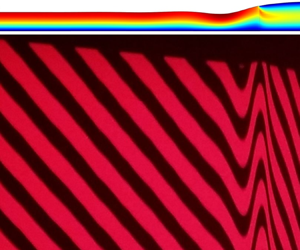
In our experiments, we used a single fringe pattern of red and black fringes, each 7 mm wide, projected onto the liquid surface. The projector's optical axis is perpendicular to the transfer zone. The curvature of the liquid surface in the hydraulic jump region deforms the fringes and works as a mirror. A single camera captures the images (figure 7a), which allows the free surface geometry to be reconstructed (red lines in figure 7b).

Figure 7. Image processing of the deformed moiré fringes. (a i) Sketch of the system (particles and film thicknesses are not to scale). (a ii) Projected moiré fringes on the free surface. (b) moiré image processing: successive steps of thresholding and gradient extraction. At the end of the image processing, the red line corresponds to the edges of the bands deformed by their reflection on the mirror constituted by the liquid surface. A geometrical optics analysis then reconstructs the hydraulic jump profiles.
4.2 Experimental results
The fringe projection profilometry described in § 4.1 allowed the surface reconstruction of the first hydraulic jump for a series of liquid flow rates. Figure 8 gives an experimental evaluation of the relative dimensionless film thickness  $H(X) - {H_N}$ in this first jump. As expected, the number and amplitude of the oscillations and the length of the first hydraulic jump in the flow direction increase with the flow rate. The results of the finite element method (FEM) calculations reported in § 5.2 will correctly corroborate these experimental features.

Figure 8. Examples of dimensionless relative film thickness profiles  $H(X) - {H_N}$ determined with the moiré technique for different values of the Reynolds number. Diameter of the particles is 280 nm. System parameter, $\varSigma \cong 0.0033$; Nusselt regime, $X < 0$. When $X \to - \infty $, $H(X) - {H_N}$ must tend to 0. Poiseuille regime, $X > 0$. When $X \to + \infty $, $H(X) - {H_N}$ must tend to ${H_P} - {H_N} \equiv 9\varSigma \,Re$.
5. Numerical simulations of the liquid film thickness profile between the feed and the second hydraulic jump
We consider the steady state, gravity-driven flow down an inclined plane channel of a Newtonian fluid. In addition, since the maximum value of the film Reynolds number is 52, turbulence plays no role, and the film flow can be considered purely laminar. The numerical simulation of the flow may rely on two approaches. The simplest one is to use a finite-difference method to solve equations (2.23) for the Nusselt regime and (2.37) for the Poiseuille regime. These two equations result from the one-dimensional (1-D) modelling of the laminar flow of the liquid film. They represent the balance between gravitational, viscous dissipation, and surface tension effects acting on the thin liquid film. Matching these two equations at  $ X = 0$ yields results identical to those obtained with the Comsol Multiphysics FEM solver of the 2-D full Navier–Stokes equations. The 1-D approach is more appealing since it is based on the film flow's essential physical features and is simpler. However, the 2-D approach provides more details on the velocity profile evolution, especially in the first hydraulic jump region. This paper only discusses simulations obtained with the Comsol Multiphysics solver.
The 2-D hydraulic jump was simulated with Comsol Multiphysics FEM solver, with the appropriate boundary conditions for the Nusselt regime (zero shear stress at the interface) and the Poiseuille regime (free normal velocity and zero tangential velocity at the particle-covered interface). A transient evolution from an approximate guess of the velocity field yields the steady-state solution of the Navier–Stokes equations. Figures 9–11 show examples of Comsol Multiphysics simulations. Figure 9 (respectively, 10) represents the x (respectively, y) component of the fluid velocity field scaled by the surface fluid velocity in the Nusselt regime. Figure 11 gives the film thickness profiles for different values of the Reynolds number. Note that the three figures should be tilted at an angle α on the horizontal. As the flow is laminar, vorticity is limited to the wall shear layers and the hydraulic jump region. Almost no vorticity is present in the bulk.

Figure 9. Dimensionless velocity field  ${u_x}/{u_{max}}$ in the liquid film across the hydraulic jump ( $X$ from −11 to +3, H from ${H_N}$ to ${H_P}$) calculated by Comsol Multiphysics FEM for $Re = 52$ (top, real scale; bottom, y scale is magnified by a factor 4); ${u_{max}}$ is the liquid interfacial velocity in the Nusselt regime. The vertical black line indicates the position $X = 0$ of the junction between the two film surface boundary conditions (free normal velocity and zero tangential velocity), i.e. corresponding to the connection between the Nusselt regime (2.23) and the Poiseuille regime (2.37).

Figure 10. Here,  ${u_y}/{u_{max}}$ FEM computed velocity field in the vicinity of the hydraulic jump ( $Re = 52$) ( $y$ scale is magnified by a factor of 4). The vertical black line indicates the position $X = 0$ of the junction between the two film surface boundary conditions (free normal velocity and zero tangential velocity), i.e. corresponding to the connection between the Nusselt regime (2.23) and the Poiseuille regime (2.37).

Figure 11. Examples of dimensionless film thickness profiles  $H(X) - {H_N}$ computed with a FEM software package for different values of the Reynolds number. Diameter of the particles is 280 nm. System parameter, $\varSigma \cong 0.0033$; Nusselt regime, $X < 0$. When $X \to - \infty $, $H(X) - {H_N}$ must tend to 0. Poiseuille regime, $X > 0$. When $X \to + \infty $, $H(X) - {H_N}$ must tend to ${H_P} - {H_N} \equiv 9\varSigma \,Re$.
In the numerical simulation (figures 9–11), the transitions in the velocity field and the film surface slope between the Nusselt and Poiseuille regimes correctly show slope discontinuities. The computed thickness profiles are fairly consistent with the measured ones. A more accurate description should probably account for the menisci attached to every particle in this transition region. However, this endeavour could be fruitless since the added complexity would be dreadful for 280 nm particles and a transition region more than 10 mm long for no anticipated significant description improvement.
The data from the confocal chromatic microscopy and the area-wide moiré topography, combined with the numerical simulations, yields without doubt that the film surface fully covered with particles behaves well as a mobile solid wall. From a fluid mechanics point of view, this almost thicknessless solid wall justifies the choice of our original boundary conditions in the Poiseuille regime, i.e. a zero tangential velocity and a free normal velocity component, only constrained by gravity and surface tension.
6. Geometric properties of the particle bed between the first and second hydraulic jumps
During the particle self-assembly into a monolayer of crystalline 2-D domains composed of grains, various defects may appear, like vacancies, dislocations, grain boundaries, stacking and disorder. These structural defects are up to reduce diffraction efficiency, increase photon scattering and generate multiple diffraction patterns due to grain boundaries.
Each grain comprises hundreds or thousands of particles organized as a hexagonal mesh with a specific planar orientation. The diffraction pattern acts as a fingerprint and reveals the structure of the colloidal monolayer, e.g. lattice spacing, average domain size, particle size distribution, defect density, etc.
To characterize the structural properties of polycrystalline colloidal monolayers at the microscopic scale, atomic force microscopy, electron microscopy (scanning electron microscopy or transmission electron microscopy), or optical microscopy are usually used. These techniques give several pieces of information, such as the degree of crystallinity, average grain size and defect patterns. However, they are not adapted to characterize the particle monolayer floating on the liquid in movement to control the assembly process in situ and in-line. The solution to obtain microscopic information about the compact film of particles on the liquid is to adopt a multiscale approach based on the diffractive response of the floating monolayer. Bragg diffraction-based techniques exploit the particle monolayer's ordered packing and periodicity to provide structural information (§ 6.1). For example, laser diffraction consists of pointing a collimated laser beam on/through the monolayer to produce a diffraction pattern that includes information on the level of organization. However, the area analysed is limited to the size of the laser spot (several square millimetres) illuminating the surface. We also developed another approach, the crystal structure mapping, that uses angular-resolved diffraction (§ 6.3). The principle is to observe several diffraction patterns at different angles of incidence with a camera and apply an image-processing algorithm to reconstruct the organization at the microscopic scale.
6.1 The Bragg diffraction topography technique
Hexagonal closed-packed particle deposits at a microscale or nanoscale have a rich palette of iridescent colours due to the diffraction of light by the HCP structure. The colours depend on the orientation of incident light, the viewing direction and the orientation of the hexagonal structure. This latter is rather homogeneous within areas of a few square millimetres, called grains, but varies significantly from one grain to another. The juxtaposition of grains on the surface thus displays a mosaic of colours, each resulting from a certain light spectrum related to the diffraction phenomenon in the corresponding angular geometry. The orientation of the particles in grains is generally studied by microscopy. Figure 12(a) illustrates this disorientation in the case of slightly deficient HCP crystallinity.

Figure 12. (a) Typical slightly irregular pattern of 1.1 μm particles, displayed by producing nanopillars on TiO2 xerogel by ultra violet insolation through nanospheres (Reference ShavdinaShavdina 2016): the white spots, actually the TiO2 nanopillars, result from the insolation of a negative resin through nanospheres. Therefore, their positions coincide with the nanosphere deposit. (b) Principle of the Bragg diffraction by a HCP film of particles. (c) Bragg diffraction rings of the white light emitted by a collimated source and impinging onto an HCP.
When a monochromatic light interacts with an HCP array of microspheres, the array acts as a diffraction grating with specific spacing between the spheres. According to the diffraction grating equation, light is diffracted at specific angles determined by the sphere diameter and wavelength of light. In the case of spheres, the diffracted light forms a pattern with hexagonal symmetry, an intense central spot from light propagating straight through or reflected and six first-order spots at an angle determined by the grating spacing. Higher-order diffracted spots can also appear but will be less intense. The diffraction pattern reveals information about the spacing and symmetry of the microsphere array. When imperfections, defects and disorder are present in the HCP array, the monochromatic diffraction pattern becomes progressively broader, less intense, less symmetric and more diffuse. The distinct spots merge into rings, indicating a loss of long-range order.
Using polychromatic light, the different wavelengths diffract at different angles. However, the hexagonal symmetry and average information about the grating spacing can still be obtained from the pattern. In this case, the colour-dispersed diffraction pattern is key to analysing the properties of the microsphere array. The experiments reported here use a white light collimated source (3150 K). The diffracted ring can be evaluated with the Bragg diffraction equation, where the refracted angle  ${\theta _r}$ depends upon the incident angle ${\theta _i}$, the diffraction order m, the component ${\lambda _l}$ of the light wavelength and the distance a between neighbouring spheres in the HCP,
 \begin{equation}\textrm{sin(}{\theta _r}) - \textrm{sin(}{\theta _i}) = m{\lambda _l}{a^{ - 1}}.\end{equation}
6.2 Experimental results on the evolution of HCP array period a and the shear stress acting on the particles with the flow rate
To extract the HCP period a from the Bragg diffraction patterns, we have developed an image-processing sequence illustrated in figure 13 and detailed in table 1. This sequence provides the averaged radius of the green fringe. A geometric optics calculation allows the determination of the incident angle  ${\theta _i}$ and the refracted angle ${\theta _r}$. The HCP period a is then calculated from (6.1).

Figure 13. Image processing to extract one component of the Bragg diffraction pattern. From (a) to (c): original image; cropped image, extracted green ring (180 × 300 pixels); fitted model.
Table 1. Image processing sequence to extract the components of the Bragg diffraction pattern.

Figure 14(a) gives the values of the HCP period a for a Reynolds number  $Re$ increasing from 12 to 52 and decreasing from 52 to 12. When the Reynolds number $Re$ increases from 12 to 52, slight compaction occurs, and the HCP period a decreases linearly from 1.113 μm at $Re = 12$ down to 1.100 μm at $Re = 52$. Afterwards, it remains roughly constant when the Reynolds number is reduced step-by-step from 52 to 12. Note that this value of 1.100 μm has been confirmed from scanning electron microscopy images and constitutes the best guess of the final HCP period. It is a highly credible value but not exact to the last digit. A simple explanation of this evolution is that the viscous shear stress under the HCP bed allows its compaction through the local reorganization of neighbour-to-neighbour interactions. In addition, when the compaction increases, the capillary forces between the particles become far more important, which maintains the compaction when the Reynolds number decreases.

Figure 14. (a) Grey circle and red line: stepwise evolution of HCP period a measured from the circle radius of the diffracted green component (circa 540 nm) filtered by averaging between nine neighbours and linear-constant trend fit during the sequence; yellow line, time sequence of the values of the Reynolds number.
(b) Same data plotted versus the dimensionless shear stress  ${T_P}$.
Remarkably, the noise of our Bragg diffraction measurements does not hide the evolution of the HCP period a. This noise is a minor consequence of the pixel size of the pictures that leads to an uncertainty of 0.0018 μm (1.8 nm) on the value of a.
As seen in figure 13bis in the supplementary material available at https://doi.org/10.1017/flo.2024.12, the diffraction pattern is only slightly sensitive to the liquid flow rate. The shear stress acting on the particles downstream of the hydraulic jump is calculated from the velocity profile given by (2.30),
 \begin{equation}{\tau _P}\,\hat{ = }\, - \mu {\left. {\frac{{\textrm{d}{u_x}}}{{\textrm{d}y}}} \right|_{y = {h_P}}} = \frac{1}{2}\rho g\,\textrm{sin}\,\alpha {h_P}.\end{equation}
Let us introduce the dimensionless quantity  ${T_P}$ that corresponds to the shear stress ${\tau _P}$ under the particle bed at $y = {h_P}$,
 \begin{equation}{T_P}\,\hat{ = }\,\frac{{{\tau _P}}}{{{\textstyle{1 \over 2}}\rho g\,\textrm{sin}\,\alpha {L_{cap}}}}.\end{equation}
 For values of the Reynolds number  $Re$ used in figure 13bis in the supplementary material (circa 17, 28 and 40 nm), the dimensionless shear stress ${T_P}$ is approximately 0.54, 0.64 and 0.71. Figure 14(a) shows the evolution of HCP period a versus ${T_P}$. Actually, capillary forces between the particles are predominant, and a more sensitive experimental approach is needed to exhibit the effect of the shear stress, as it will be shown in the following. However, it has been verified experimentally that the lowest values of the Reynolds number within the range of possible values ( $Re = 6$, 12 and 17) are less efficient in assembling the particle. In contrast, $Re$ values of 28, 34 or 40 are more potent. The higher $Re$ values of 46 and 52 are usually less used due to the occurrence of a wavier film flow regime.
6.3 Experimental results on the HCP crystal structure mapping
At the macroscopic scale, according to previous work (Reference Delléa, Shavdina, Fugier, Coronel, Ollier, Désage and RatchevDelléa et al. 2014), six images of the sample observed at normal incidence illuminated under six different incidence angles are needed to obtain a diffraction pattern (figure 15). The image processing consists of comparing the six images and eventually subdivisions of these images to sharpen the analysis (the decision process is briefly presented in table 2). Finally, the software programs constitute artificial images of particle deposits, giving significant information about grain size, grain morphology, orientation distributions, defaults (voids, stacking), etc, at microscopic and macroscopic scales. With these new control methods, colloidal lithography is emerging as an industrial process.

Figure 15. (a) Set of six views of the same zone, illuminated at six different angles (0°, 10° 20°, 30°, 40°, 50°) to enlighten the 2-D colloidal crystal structure. (b) The same six images converted to greyscale. (c) The false-colour image obtained with coding classes 1 to 7 defined in table 2 from 1 = blue to 7 = red.
Table 2. Image processing sequence to classify the different zones of the 2-D crystal.

The particle film is usually constituted of grains with a wide variety of sizes and forms. They are arranged randomly due to the local hydrodynamic and capillary forces. Each grain is a crystalline domain with a hexagonal compact mesh and its specific orientation on the liquid surface. When illuminated with white light, each grain diffracts the incident light in six space directions. For a punctual observation, the black zones correspond to grains whose diffraction is in another direction.
To progress towards automating or industrializing the process, it is very important to quantify, dynamically and in real time, the particle organization on large macroscopic zones (at least several square centimetres). Moreover, as the assembling technique is based on a free-flowing liquid, this optical contactless measurement capability is an essential advantage compared with the classical quasistatic original LB process. This capability allows dynamic control of the particle assembly process parameters (e.g. Reference Delléa, Desage and FugierDelléa, Desage & Fugier 2013). Correcting the defective or non-compliant zones directly at the liquid surface is also possible by removing specific zones with a vacuum system before the final transfer onto a substrate. The production of large samples can strongly benefit from this new strategy for optimizing process control conditions.
7. Synthesis of the results
This work focused on an innovative system that could continuously create large crystalline structures on theoretically unlimited substrate sizes. The innovative system is far more effective than the LB original method.
We used four optical techniques to analyse the different aspects of the liquid film flow, especially the film thickness evolution and the first hydraulic jump, the impact of the liquid flow on the particle bed and the resulting particle deposit.
Our experiments validated the semiparabolic and parabolic velocity profiles in the liquid film. To our knowledge, the boundary condition at the film interface in the Poiseuille regime (zero velocity tangential components, free velocity normal component) has never been used before in theoretical analyses or numerical simulations of liquid film flows.
The original LB approach requires a great deal of skill to prevent the stacking of particles into a multiple layer. In contrast, in our flow design involving an inclined ramp, the flow rate can control the viscous stress on the particles softly and progressively.
Another advantage of our ramp design is that the deposition process on the ramp can be continuously monitored using our HCP crystal structure mapping.
To conclude, the technological spin-offs of our experimental, theoretical and numerical results will unquestionably help design equipment for industrial-scale production. Indeed, mastering all the control parameters allows dynamical fine-tuning of the assembly process and optical control of the quality of the HCP before it is transferred onto a final solid substrate. Our approach is multiscale since knowledge of the optical response to diffraction from submicron structures can be used to deduce the morphology of the crystal structure at macroscopic dimensions.
Colloidal crystallization is still challenging, with the aim of producing colloidal single crystals on large surfaces with perfect HCP ordering on large areas.
Supplementary material
Supplementary material is available at https://doi.org/10.1017/flo.2024.12.
Funding statement
This research was supported by CEA/Liten.
Declaration of interests
The authors declare no conflict of interest.
Author contributions
Optical measurements, O.D; dimensional analysis and scaling, J.M.D; fluid mechanics modelling, O.L; Bragg diffraction data reduction, O.L; writing original draft, O.L, J.M.D, O.D. All authors approved the final submitted draft.


 Open access