1. Introduction

In Alpine countries avalanche-dynamics models are used by engineers and land-use planners to predict the reach and destructive force of snow avalanches. For the past 40 years the Voellmy model (Reference VoellmyVoellmy, 1955). with major modifications made by Reference SalmSalm (1966, Reference Salm1972). has been applied to dimension avalanche-hazard zones in Switzerland. The Voellmy–Salm (VS) model is embedded in the Swiss Guidelines for avalanche runout calculation (Reference Salm, Burkard. and Gubler.Salm and others, 1990). The model (and the Swiss Guidelines) have often been criticized in the literature. Some of the most frequent complaints are:

1. 1. the VS model is incomplete since it calculates neither the dispersal of the snow mass as it moves down the mountainside, nor the instantaneous velocity field, nor the deposition area in the runout zone (Reference Hutter, Savage. and Nohguchi.Hutter and others, 1989);

2. 2. the runout distance is calculated with respect to the center of mass and not the leading edge of the avalanche (Reference McClung and Mears.McClung and Mears, 1995);

3. 3. the predicted deposition heights are unrealistic (Reference McClung and Mears.McClung and Mears, 1995).

4. 4. it is illogical to compute avalanche velocities and runout distances on paths of complex geometry by selecting a priori the reference position that separates the acceleration and deceleration portions of the avalanche path (Reference Perla, Cheng. and McClung.Perla and others, 1980);

5. 5. the VS model takes into account only the external forces acting on the avalanche mass and does not provide information on the distribution of stresses within the avalanche body (Reference Norem, Irgens. and Schieldrop.Norem and others, 1989).

Because of these deficiencies, a detailed verification of the VS model using experimentally measured velocities and flow heights is not possible. A description of the VS calculation procedure and a thorough critique — and defense — of the VS model can be found in Reference Bartelt and Gruber.Bartelt and Gruber (1997).

The purpose of this paper is to present a quasi-one-dimensional, hydraulics-based, depth-averaged continuum model that resolves the above-listed shortcomings and therefore provides a more detailed description of avalanche motion. The model continues to employ a Voellmy-fluid flow law. This law divides avalanche flow resistance into a dry Coulomb-type friction and a viscous resistance which varies with the square of the flow velocity.Footnote ¹ Voellmy termed the latter “turbulent” friction since the mathematical formulation is similar to the well-known turbulent Chezy equation used in open-channel-flow hydraulics. Voellmy also considered non-rectangular velocity profiles, implying that he believed that large shear deformations exist within the avalanche flow body (see Reference VoellmyVoellmy, 1955).

These notions, however, have not been supported by experimental evidence or observations of real avalanches (Reference Gubler, Miller., Klausegger. and Suter.Gubler and others, 1986). The “turbulent” friction term has been redefined as a shear resistance acting at the sliding base of the avalanche. According to Reference SalmSalm (1993), the resistance is due to the impact of moving snow granules with obstacles protruding from the ground, which continuously dissipates kinetic energy. The protrusions may have dimensions of 0.1–1.0 m. The shear layer where these collisions occur is small compared to the total flow height, especially for large avalanche events. On an absolutely flat sliding surface the “turbulent” friction term disappears (see the fast observed acceleration of snow avalanches in starting zones). The avalanche body contains no shearing deformations and moves as a cohesive “plug”. Thus, the physical interpretation of the Voellmy-fluid resistance law has undergone considerable transformation since the original definition was proposed by Voellmy.

Voellmy also did not introduce internal friction into his model, because he believed that the “turbulent movement” of the avalanche substantially reduces flow resistance in a process similar to “the vibrating of concrete to improve its workability”. However, Reference SalmSalm (1968) maintained that snow is not an ideal fluid and, subsequently, under a tensile (active) or compressive (passive) longitudinal strain, internal friction arises. He proposed that the longitudinal stress depends only on the internal friction angle, as in dry sand. The magnitude of the internal friction angle was first based on measurements (angle of repose) of avalanche deposits, and then on actual experiments with the snow chute of the Weissfluhjoch (Reference SalmSalm, 1968). This simple model allows for active/passive longitudinal straining in the flow plug which regulates flow heights primarily in the transition zone. This concept has also been introduced into the numerical model, which likewise regulates flow heights. It introduces a third flow parameter into the model (termed the active/passive pressure coefficient, λ), but one that, compared to the Voellmy-fluid parameters, does not vary significantly. This simple procedure avoids the introduction of more than one additional flow parameter. In reality, cohesion also plays an important role (see, e.g., the behavior of avalanches in the runout zone). In this case, the internal friction should consist of two parts, one based on the friction angle and the other on the cohesion. Since only the first part is contained in the VS model and other numerical models, such as Reference Savage and Hutter.Savage and Hutter (1991) or the proposed one, this fact appears as an increase in λ during the back-calculation of real avalanches.

Nonetheless, an essential question to pose is why newer numerical models should continue to employ an old and perhaps outdated flow law. Detractors of Voellmy-fluid models assert that the model is purely phenomenological, i.e. the model parameters are based solely on back-calculations of field events. As such, the model parameters cannot be measured independently. Numerical models could employ flow laws based on constitutive equations formulated from both field and laboratory tests. A first step in this direction is the Norwegian NIS (Norem, Irgens and Schieldrop) model based on a modified Criminale–Erickson–Filby constitutive flow law (Reference Norem, Irgens. and Schieldrop.Norem and others, 1987). This constitutive law agrees with Bagnold’s theory of granular flow, in that both the shear and normal stress vary with the square of the shear rate. At the very least, a model should be able to simulate laboratory chute experiments, as in Reference Hutter, Koch., Plüss and Savage.Hutter and others (1995).

Advocates of Voellmy-fluid models counter by arguing that, first of all, most models, including the NIS model, define the sliding friction between the ground and the avalanche body as the sum of a Coulomb-type friction and a term proportional to the flow velocity squared: (Reference Perla, Cheng. and McClung.Perla and others, 1980; Reference Norem, Irgens. and Schieldrop.Norem and others, 1987, Reference Norem, Irgens. and Schieldrop.1989; Reference Kumar, Sharma., Mathur. and HestnesKumar and others, 1998; Reference Grigorian and Ostoumov.Grigorian and Ostoumov, in press). Several of these models have also been validated by extensive comparison to field events (e.g. the Russian model; Reference Eglit and HestnesEglit, 1998). Secondly, an important assumption of the Voellmy-fluid model, which has been verified by field tests, is plug flow. Due to cohesion and the fast sintering of snow granules in the main part of flow, there is no possibility of snow-particle motions relative to neighboring particles. In the shear layer, particle motion is restricted; the mean free path of these particles is very small. Therefore, a constant particle concentration and a rectangular velocity profile can be assumed. In general, and especially in the runout zone, advocates do not believe in the fluidization of the entire avalanche body. Particles (not single ice crystals but snow clods with diameters of 0.1–1.0 m) have coefficients of restitution close to zero. This impedes the upward movement of the snow granules; moreover, the granules move with a stream-wise velocity: a necessary physical and mathematical condition for the depth integration of the governing differential equations and the formulation of any hydraulic model.

Another argument is the lack of well-tested alternatives. Models which divide avalanche flow into both a plug-f1ow and a fluidized layer regime are too complicated, and are hampered by the need for correct definition of the fluidized layer height. In our simulations using the Norwegian NIS model, which at present assumes no plug-flow regime, we have found that the model can satisfactorily simulate many-extreme avalanche events, but that the shear deformations within the avalanche body are unrealistically large (Reference Bartelt, Salm. and HestnesBartelt and Salm, 1998).

Finally, proponents of the Voellmy-fluid model (Reference SalmSalm, 1993) point out that the model is not based on laboratory tests and computer simulations with materials which are completely different from snow, such as glass spheres, crushed walnut shells or plastic. The Voellmy-fluid law is based on observations of real avalanches. In the end it is a simple model, perhaps too simple, but the complexity of the avalanche-dynamics problem demands simplification.

These arguments are not entirely convincing. Opponents say that more hard evidence is required. For example, the model parameters are based on comparing runout distances of real avalanche events alone. As stated above, very little work has been done to corroborate measured flow velocities and deposition heights. Even the velocity and flow-height measurements of a well-documented extreme avalanche like Aulta (Reference Gubler, Miller., Klausegger. and Suter.Gubler and others, 1986) are inadequate to test the model’s flow assumptions because of the very rough estimate of the initial fracture volume of the avalanche.

This is a very interesting, and unresolved, scientific debate which has an important practical component: a special advantage of the Voellmy-f1uid flow law is that it contains only two flow parameters whose magnitude has been determined by back-calculations using historical avalanche events (Reference Buser and Frutiger.Buser and Frutiger, 1980). This set of well-calibrated flow parameters for extreme avalanche events is a necessary condition for the application of any newer (numerical) model in practice.

Thus the second aim of this paper is to clearly evaluate the use of a numerical Voellmy-fluid flow law for practical avalanche-dynamics calculations. We begin by stating the governing differential equations of the numerical Voellmy-fluid model in section 2. We state the equations in general conservative form, which allows us to apply upwinded finite-difference schemes that contain no artificial numerical damping. Unlike previous attempts to solve this problem (Reference Hutter, Koch., Plüss and Savage.Hutter and others, 1995), the integration scheme is Eulerian. We regard this as an important first step in developing a robust quasi-two-dimensional model that can be employed in a three-dimensional terrain. Such a model would have many uses in practical avalanche-dynamics calculations, including the determination of the height and location of avalanche-deflecting dams (Reference Gruber, Bartelt., Haefner. and HestnesGruber and others, 1998).

The righthand side of the governing differential equations is formulated generally in terms of the friction slope, S _f (for an exact definition see Equation (9)), and the active/passive pressure parameter, λ. Based on the work of Reference Bartelt, Salm. and HestnesBartelt and Salm (1998), we briefly state these values for the NIS model. Russian researchers (Grigorian and Ostoumov, 1995; Reference Eglit and HestnesEglit, 1998) have also proposed a modified Voellmy-fluid law in which the dry-friction term of the Voellmy fluid is limited by a yield stress. The model, however, does not distinguish between active and passive flow states. The friction slope for this model is stated and briefly discussed.

The Voellmy-fluid model is applied to simulate a laboratory chute experiment documented in Reference Hutter, Koch., Plüss and Savage.Hutter and others (1995). Then an extreme avalanche event, Ariefa/Samedan, is simulated with flow parameters close to the values recommended by the Swiss Guidelines. To deflect criticism that Swiss researchers are not prepared to investigate other flowing-avalanche models, we compare the Voellmy-fluid model with the Russian yield-stress model and the Norwegian NIS model on the Mettlenruns test track. It is difficult, if not impossible, to apply the older VS model in Mettlenruns because there is no clear transition (point P) between the avalanche track and runout zone.

As the VS model is so widely used (not only in Switzerland), it is of great interest to determine the conditions under which it will provide correct and reliable results. Most avalanche-hazard maps in Switzerland and elsewhere have been calculated with the VS model. Since building projects may he affected, the results of the VS model have important financial implications. There is therefore an urgent need to evaluate the application limits of the simplified VS model by comparing simulation results to a more complex numerical model. Since, in practical applications, all avalanche-dynamics models require the specification of initial flow conditions, the influence of initial fracture dimensions on predicted runout distances is investigated in section 7. The analysis is similar to Reference McClung and Mears.McClung and Mears’ (1995) investigation. We show the conditions under which the results of the numerical Voellmy-fluid model will converge with the traditional VS model. This section underscores the importance of the initial conditions and the difficulties of applying numerical methods in practice. It also indicates how snow-avalanche calculation guidelines must be modified in order to apply any numerical model for practical avalanche-runout calculations.

2. A Voellmy-Fluid Model

Let X be the horizontal coordinate and Z(X) the mountain profile. The formulation of our quasi-one-dimensional depth-averaged continuum model uses the independent variable x to define the length along the avalanche profile (see Fig. 1). Avalanche flow is described by two scalar fields A(x, t) and Q(x, t). The first field, A(x, t), represents the cross-sectional flow area at x and time t, and the second field, Q(x, t), gives the average snow discharge along the mountain profile. The principles of conservation of mass and momentum are invoked to provide the governing differential equations describing dense-snow avalanche movement in conservative form:

(1)

. (2)

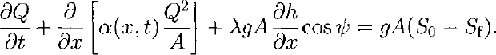
As usual, g is acceleration due to gravity, h(x, t) is the avalanche flow height, S ₀ and S _f are the acceleration and friction slope, respectively, λ is the active/passive pressure coefficient and α is the velocity profile factor. The equations are based on several important assumptions:

1. 1. Flowing snow is modeled as a fluid continuum of mean constant density ρ.

2. 2. The flow width, w(x), is known.

3. 3. A clearly defined top flow surface exists.

4. 4. The flow height, h(x, t), is the average flow height across the section, i.e. the flow height is level over the flow width, w(x).

5. 5. The vertical pressure distribution is hydrostatic. Centripetal pressures which modify the hydrostatic pressure distribution are not accounted for.

6. 6. Flow velocity and depth are unsteady and non-uniform.

Note that the system of equations is completely general; no assumptions have yet been made regarding the constitutive relations, slip conditions or velocity profile.

Fig. 1. Voellmy fluid.

The parameter α(x, t) is the velocity profile factor. For a rectangular velocity profile,

. (3)

See Reference Savage and Hutter.Savage and Hutter (1989) for more details.

We call S ₀ the acceleration slope. It is given by

(4)

where ψ(x) is the inclination of the mountain slope from the horizontal. The friction slope, S _f, is found by depth-averaging the shear stress gradient:

. (5)

In our definition of a Voellmy fluid, we assume that no shearing deformations γ occur in the avalanche body and at the top surface:

. (6)

The avalanche moves as a plug with a velocity that is constant over the depth of flow, h (see Fig. 1). No fluidized shear layer exists since shear deformations are concentrated at the base of the avalanche; the shear layer is considered small compared to the avalanche flow height. The basal shear resistance consists of a dry Coulomb-like friction and a Chezy-like resistance:

. (7)

The stress σ _z is the overburden pressure at z = 0 and is dependent on the flow height:

. (8)

Implicit in this definition is the assumption of a hydrostatic pressure distribution. U is the flow velocity of the plug. The parameters μ and (m s²) are constants whose magnitude depends, respectively, on snow properties and the roughness of the flow surface. See Reference Salm, Burkard. and Gubler.Salm and others (1990) or Reference SalmSalm (1993) for a more detailed explanation.

The friction slope for a Voellmy fluid is subsequently

. (9)

Although no shearing deformations occur within the avalanche body, the flow plug will certainly undergo considerable longitudinal straining. The stress in the longitudinal direction is proportional to the hydrostatic pressure and is given by

(10)

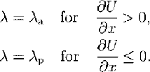
where λ is the so-called active/passive pressure coefficient. We discriminate between active (tensile) and passive (compressive) cases based on sign of the velocity gradient (strain rate) in the longitudinal direction, ∂U/∂x,

. (11)

This definition allows different amounts of internal flow friction to be introduced depending on whether the plug is being longitudinally pulled apart (e.g. in the release zone) or compressed (e.g. in the runout zone). Rankine’s theory is applied to define the active/passive pressure coefficients:

. (12)

φ is the internal friction angle, closely related to the angle of repose of snow. Typical values are in the range 20° ≤ φ ≤ 40°, leading to active/passive pressure values in the range 0.2 ≤ λ_a ≤ 0.5 and 2.0 ≤ λ_ρ ≤ 4.6. Alternative definitions of the active/passive pressure values are possible (Reference Hutter, Koch., Plüss and Savage.Hutter and others, 1995; Reference McClung and Mears.McClung and Mears, 1995). This simple formulation neglects the influence of slope angle, φ, dry friction, μ, and cohesion on the active/passive coefficient.

This model of avalanche flow clearly oversimplifies a very complex granular movement, especially in cases where a larger fluidized layer exists (e.g. when an avalanche flows into a narrow gully). These effects are taken into account by-reducing , as in open-channel-flow hydraulics.

Alternative flow laws can be introduced into the model. These will be discussed in the following sections. The differential equations are solved numerically using first- and second-order upwinded finite-difference schemes. For details see Reference Sartoris and Bartelt.Sartoris and Bartelt (in press).

3. Russian Modifications to the Voellmy-Fluid Model

Since the late 1960s, Russian researchers, primarily M. Eglit and S. Grigorian at Moscow State University, have used depth-averaged continuum models to simulate dense-snow avalanche flow. For an overview of this work see Reference Bozhinskiy and Losev.Bozhinskiy and Losev (1987) or Reference Eglit and HestnesEglit (1998). These models have been constructed based on observations and measurements of real avalanche events in the Caucasus and Khibiny mountain ranges. The Russian implementation of the Voellmy-fluid model differs from the Swiss model in two important aspects.

Firstly, the Coulomb friction law was modified by introducing an upper limit on the dry friction. Moreover, the shear stress at the base of the avalanche is

. (13)

The height, h _y, is the critical snow height at which yielding at the basal surface occurs:

. (14)

The stress τ _y represents the minimal shear strength, or yield stress, of the sliding surface. Physically, this law implies that the friction force cannot increase indefinitely with an increase in normal stress, i.e. an increase in flow depth. The shear stress on the interface between the avalanche and sliding surface reaches the yield stress and cannot increase further.

Secondly, the Russian model does not distinguish between active and passive flow states:

. (15)

In summary, the friction slope for the Russian Voellmy-fluid model is

. (16)

This law was introduced to explain the fact that large avalanches can travel long distances and simulation with the standard Voellmy-fluid model produces unsatisfactory results. This fact is evident in the Swiss Guidelines which state that different μ values are to be used for small (μ = 0.300) and large (μ = 0.155) avalanches. Both these values are significantly smaller than measured dry-friction values (see, e.g., Reference Dent, Burrell., Schmidt., Louge., Adams. and Jazbutis.Dent and others, 1998). This model assumption thus explains why flow friction decreases with avalanche size (Reference Bozhinskiy and Losev.Bozhinskiy and Losev, 1987).

4. The Norwegian NIS Model

The NIS model is described in Reference Norem, Irgens. and Schieldrop.Norem and others (1987, Reference Norem, Irgens. and Schieldrop.1989). It is based on the idea of using a modified Criminale–Ericksen–Filby fluid to model avalanching snow. Although the constitutive equations contain a cohesion term, all implementations to date assume that the avalanching snow is completely cohesionless. The introduction of cohesion is not possible without finding a suitable definition of the fluidized layer height. A reformulation of the model, again assuming that avalanching snow is cohesionless, is described in Reference Bartelt, Salm. and HestnesBartelt and Salm (1998). The aim of this section is to briefly present the model, highlighting the important differences from and similarities to the Voellmy-fluid model, so that the reader can understand the upcoming model comparison.

The main difference between the NIS and Voellmy-fluid models is that the NIS model contains no plug-flow regime. The velocity profile, shown in Figure 2, is not constant. The velocity at the base of the avalanche, u ₀, is different from that at the top surface, u _h. The velocity profile factor is

. (17)

The avalanche flow body is completely fluidized.

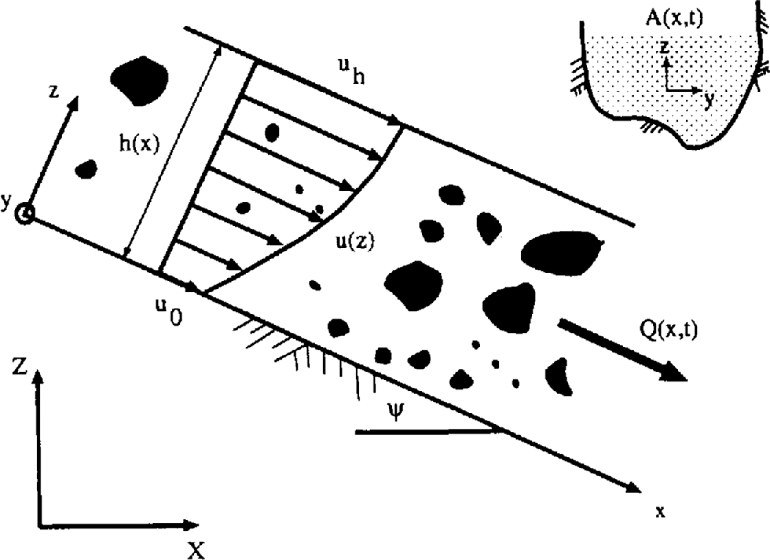
Fig. 2. Vertical velocity profile assumed in the NIS model. Definition of flow variables.

The model contains five flow parameters, b, s, m, v ₁ and v ₂, where b is the coefficient of dry friction (μ), s is the velocity-squared dynamic-friction parameter (s = ρg/), which like is dependent on surface roughness, m is the shear viscosity and ν ₁ and ν ₂ are the normal stress viscosities. The ratio R between the upper and lower velocities is given by

. (18)

Note that when s = 0 (i.e. the surface is perfectly smooth), u ₀ = u _h and the velocity profile is rectangular, α = 1. This physically implies that fluidization of the avalanche body is caused by terrain roughness.

Sliding resistance at the avalanche base is given by a Voellmy-fluid law, so it is not surprising that that the NIS friction slope is similar to the Voellmy-fluid friction slope but contains an additional term accounting for internal flow resistance:

. (19)

Note that the internal friction is a function of the longitudinal strain rate ∂(u _h – u ₀)/∂x. Also, the viscous drag term is a function of the velocity at the base of the avalanche, u ₀, which may differ significantly from the mean flow velocity, U, of the avalanche,

. (20)

Finally, the passive pressure is given by

. (21)

Thus, in contrast to the Voellmy-fluid model, the distinction between active and passive flow states is made in the friction slope, and not in the “passive” pressure parameter, λ. A nice feature of the NIS model is that it includes a mechanism to introduce different amounts of internal friction based on the longitudinal strain rate. Instead of being introduced in an ad hoc way, as in our Voellmy-fluid model, this is introduced via a set of constitutive equations.

For a complete description of these terms see Reference Norem, Irgens. and Schieldrop.Norem and others (1987, Reference Norem, Irgens. and Schieldrop.1989) or Reference Bartelt, Gruber. and Salm.Bartelt and others (1998).

5. A Laboratory Chute Experiment and a Field Case-Study

Well-documented observations of snow avalanche events are rare. For this reason, laboratory chute experiments have been carried out to validate granular flow models (Reference Hutter, Koch., Plüss and Savage.Hutter and others, 1995). Chute experiments have the advantage that the initial fracture conditions, geometry of the avalanche track and properties of the flow materials are well defined. The disadvantage is that the cohesionless flow materials are not like snow. In this section, one of the many laboratory experiments published in Reference Hutter, Koch., Plüss and Savage.Hutter and others (1995) will be simulated using the proposed model.

The laboratory chute consists of two straight 100 mm wide track segments separated by a short transition zone. In our experiment, 4 kg of glass beads were released down the first track segment which was inclined at 60° (experiment 117). The second track segment was flat. The track geometry is shown in Figure 3. The chute was lined with drawing paper to increase the basal friction. The glass beads were 3 mm in diameter. High-speed photography was used to determine the position of the avalanche as a function of time. Full information, including a series of photographs of the event, can be found in Reference Hutter, Koch., Plüss and Savage.Hutter and others (1995).

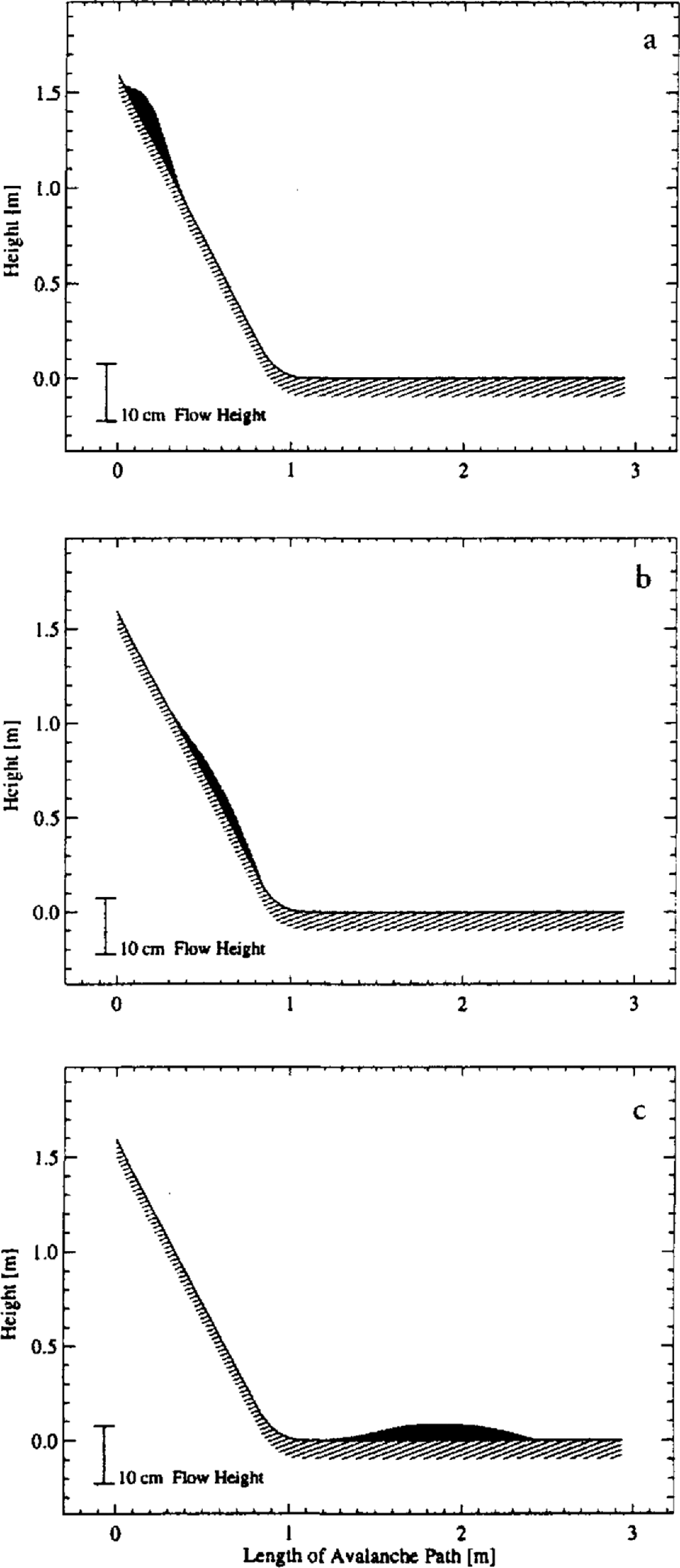
Fig. 3. Computer simulation of a laboratory chute experiment in which 4 kg of glass beads were released down a 60° inclined chute. (a) Shortly after release; (b) transition zone; (c) at-rest position. The flow heights are increased by a factor if 3. The final deposition form agrees well with the experimental results. Simulation parameters: μ = 0.49, ø = 26° and = 2000 m s⁻².

Figure 3 shows the simulated avalanche at various locations on the track. After release, it accelerates to a terminal velocity of 3.5 m s¹ before coming to rest on the flat track segment. The calculated runout distance agrees well with the experimental value.

In Figure 4 the calculated and experimental positions of the front, rear and maximum height are displayed. Good agreement exists for both the front and rear positions. The calculated location of the maximum flow height is nearer to the avalanche front than observed in the experiments. This position is sensitive to the initial conditions, especially the initial shape of the mass. In the simulations a rectangular mass with a constant height was released with an initial velocity of 2 m s⁻¹. This assumption may not reflect the true shape of the mass after it has been released.

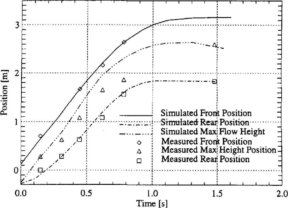
Fig. 4. Comparison between measured front, rear and maximum height positions and computer simulation shown in Figure 3. Simulation parameters: μ = 0.49, ø = 26° and ζ= 2000 m s⁻².

Previous simulations of this experiment use a Lagrangian finite-difference model with artificial diffusion (Reference Hutter, Koch., Plüss and Savage.Hutter and others, 1995). Hutter’s model does not employ a viscous friction to decelerate the flow mass. Instead only a basal Coulomb-type friction and an active/passive internal friction are used. These two friction terms are also employed in our model. In fact, the magnitude of the friction parameters did not differ from those employed in the Lagrangian model (μ = 0.49 and ø = 26°). However, in contrast to the Lagrangian model, viscous friction had to be introduced to regulate the flow velocities. Without viscous friction, the model avalanche flowed past the end of the chute. A value of ζ= 2000 m s⁻² was used in our model to stop the avalanche at the correct location.

The avalanche event used to demonstrate the application of the numerical Voellmy-fluid model in practice is one of the four calculation examples of the Swiss Guidelines: the Ariefa avalanche that occurred in early January 1951 during the catastrophic avalanche in Samedan, Canton Grisons, Switzerland. This event is often used to test avalanche-dynamics models (Reference SalmSalm, 1993; Reference McClung and Mears.McClung and Mears, 1995; Reference Bartelt, Gruber. and Salm.Bartelt and Gruber, 1997) because the terrain is ideal (see Fig. 5). The avalanche profile consists of two track segments of nearly constant slope and width. The transition zone between the avalanche track and runout zone is well defined. Subsequently, the track is suitable for analytical methods and a good first field example to test the proposed numerical model. More field examples can be found in Reference Bartelt, Gruber. and Salm.Bartelt and others (1997).

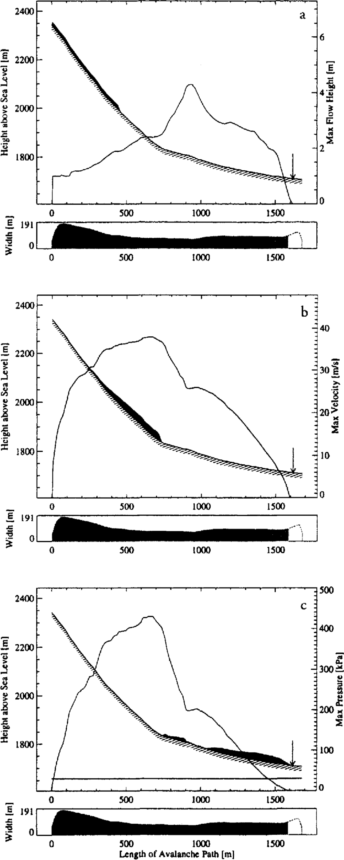
Fig. 5. The Ariefa/Samedan avalanche. Predicted avalanche flow heights (a) in the release zone, (b) in the transition zone, (c) in the runout zone. (b) also depicts maximum flow velocities over the length of the avalanche track. (c) also shows simulated dynamic impact pressures. The simulated avalanche reaches a terminal velocity of >30 m s⁻¹ and travels > 1.5km in 60 seconds. The flow heights are increased by a factor of 15. The arrow marks the measured runout distance.

The avalanche fracture zone was large; it extended between 2000 and 2350 m a.s.l. and was 100–180 m wide. A constant snowpack fracture-height of 1 m was specified following the Swiss Guideline recommendations for regional fracture depths, which are statistically related to extreme-precipitation periods. The avalanche fracture volume was > 70 000 m³ of snow. The well-calibrated Swiss Guideline friction values (see Reference Salm, Burkard. and Gubler.Salm and others, 1990) for extreme avalanche events, μ = 0.155 and λ_p = 2.5, were specified for the simulations. A slightly larger viscous drag coefficient, = 2000 m s⁻², was chosen to offset the smaller (and more realistic) flow heights computed by the numerical model (see Reference Bartelt, Gruber. and Salm.Bartelt and others (1997) for a full explanation). All friction values remained constant, in time and space, for the entire avalanche event.

Figure 5 depicts the numerical avalanche at various stages of its motion down the mountainside: in the release zone (Fig. 5a; the avalanche starts from rest), in the transition zone (Fig. 5b; the flow heights are over 2 m) and in the runout zone (Fig. 5c; the avalanche is deposited over a length of 500 m). The avalanche deposits on the flat track segment near the transition zone cannot be predicted with the VS model. In each plot the predefined avalanche flow width is shown. There is good agreement between measured and predicted avalanche runout. The Swiss Guidelines predict a flow velocity of 26.5 m s⁻¹ in the transition zone; the numerical model predicts 37.0 m s⁻¹. The shaded region in the track-width profile also shows the predicted high-hazard red zone (dynamic pressures >30kPa) and moderate-hazard blue zone (dynamic pressures ˂30 kPa). This information is used by land-use planners when preparing hazard maps. Finally, the model predicts 2.0 m deposition heights, significantly smaller than the 9.0 m depositions predicted by the Swiss Guidelines. The actual avalanche deposition heights were not recorded.

6. Model Comparison: Mettlenruns

The avalanche track we have chosen to compare the three different models is Mettlenruns, located near the village of Engi, Canton Glarus, Switzerland. In 1960 our research institute installed a pressure-measurement panel in the runout zone of this track at 910 m a.s.l. During winter 1974–75 several ropes were strung across the avalanche path in order to determine the flow velocity in front of the panel. Since the distance between the ropes is known as well as the time required for the avalanche to reach each rope, the flow velocity can be estimated. Between 1962 and 1992 all large avalanche events in this test region were observed by the local forester, Mr H. Marti, who noted the date, type of avalanche and weather conditions. Weather permitting, he also made sketches of the avalanche perimeter and estimated the fracture depth. In the following we are interested in a large wet-snow avalanche that occurred in stormy weather on 29 December 1974.

The Mettlenruns track and this particular avalanche are interesting for several reasons:

1. 1. The VS method is difficult to apply because the track consists of a long slope of almost constant angle (mean slope angle ≈28°). There is no well-defined runout zone, and point P, the location of the avalanche’s terminal velocity, is impossible to define (see Fig. 6). It is an ideal track for demonstrating the advantages of any numerical model.

2. 2. The runout distance as well as the flow velocity (18 m s⁻¹) and flow height (8 m) at the measurement panel are known. The flow height was determined by studying the flow channel after the avalanche event.

3. 3. The entire snowpack fractured, i.e. the avalanche was a ground avalanche. The total snowpack height was known and the fracture zone was sketched by the forester. Hence, the initial fracture conditions, h ₀ = 2.80 m, t ₀ = 150 m and V ₀ = 77 700 m³, are rough but reliable estimates.

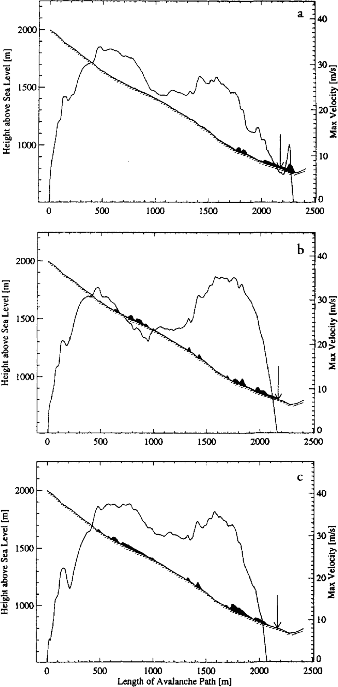
Fig. 6. Computer simulation of Mettlenruns avalanche, showing maximum flow velocities. (a) Voellmy-fluid model; (b) Russian yield-stress model; (c) Norwegian NIS model. The flow heights are increased by a factor of 15. The arrow marks the observed runout position. The measurement panel is located at 910 m a.s.l.

Our goal in this analysis is not to find the parameter combination that best fits the measurements and observations. This can easily be achieved with all three models. Instead we want to approach the problem from a practical standpoint, i.e. supposing we had the task of protecting several buildings, say a ski-lift, in the runout zone. The goal of such an analysis is to find out if the buildings can be reached by an avalanche, and, if so, its size and velocity, so that maximum impact pressures can be estimated. Furthermore, since defense strategies often involve deflector dams, information regarding the flow heights is sought. Sometimes snow deposited behind dams must be cleared by the (ski-lift) owner to ensure the effectiveness of the dam. This information is required in order to compare the cost-efficiency of different avalanche defense solutions.

The Mettlenruns track is very atypical because information on the flow velocities, flow heights and even initial conditions is known. The avalanche profile and flow width have also been documented and will be used in the analysis. Usually an analyst does not have this information. The analyst must rely on his/her experience to select the avalanche flow width and fracture area. In Switzerland, the Guidelines define a procedure for estimating the initial fracture height. If previous avalanches were recorded, the analyst might be able to assess the maximum runout distance. Not knowing the initial fracture volume, however, makes even the runout information uncertain.

For the Voellmy-fluid model we will apply the recommended parameters of the Swiss Guidelines for wet-snow avalanches at this elevation: μ = 0.300, = 1000 m s⁻² and λ = 2.5. No other parameter combination will be tested.

For the Russian model we will use τ _y/ρ values reported in Reference Eglit and HestnesEglit (1998) to model avalanches in the Elbrus (central Caucasus) and Khibiny mountain ranges. There are in the range 6.0 m²/s² ≤ τ _y/ρ ≤ 10.0m²/s². Note that in Reference Dent and Lang.Dent and Lang (1983) and Reference Lang and Dent.Lang and Dent (1983) τ _y/ρ ratios in the range 1.5 m²/s² ≤ τ _y/ρ ≤ 3.0 m²/s² were found when back-calculating slow-moving (dry) avalanche events (velocities ˂20 m s¹) with a biviscous modified Bingham model. We will employ τ _y/ρ = 8.0 m²/s², a value in the middle of the range of values found by Eglit. It is possible to use higher yield stresses, but then the model does not differ from the Voellmy-fluid model, since the yield stress is never reached. The same dynamic-friction value, = 1000 m s⁻², of the Voellmy-fluid model and Swiss Guidelines will be used. A higher but experimentally verified dry-friction value, μ = 0.42 (Reference Dent, Burrell., Schmidt., Louge., Adams. and Jazbutis.Dent and others, 1998), will be used with the Russian model. This value is also within the range used by Reference Eglit and HestnesEglit (1998).

The Norwegian model is much more difficult to apply since information on suitable parameter values is not available. We have found that the parameter combination, m = 0.002 m², b = 0.30, s = 0.5 kg m³, ν ₁/ν ₂ = 10 and m/ ν ₂ = 1, models not only the well-documented Aulta avalanche well, but also the extreme avalanches of the Swiss Guidelines (Reference Bartelt, Salm. and HestnesBartelt and Salm, 1998); for the Mettlenruns track, however, these values provide unrealistically large flow velocities and runout distances. Lacking any alternative, we will take the parameter combination which matched the runout distance best: m = 0.01 m², b = 0.50, s = 2.0 kg m³, ν₁/ν₂ = 10 and m/ν ₂ = 1. These values differ significantly from the extreme parameter combination: the shear viscosity m and dynamic friction s have increased five and four times, respectively.

The results (velocities and maximum flow heights) of the computer simulations are shown in Figures 6 and 7. The Voellmy-fluid model overestimates the runout distance and slightly underestimates (15 m s¹) the flow velocity at the measurement panel (18 m s⁻¹). The observed flow height at the panel (8 m) is severely underestimated (3 m). The Voellmy-fluid model also predicts that the entire fracture volume is deposited in the runout zone; there are no track depositions. This is clearly because the dry-friction value (μ = 0.30) is much smaller than the tangent of the mean slope angle (tan ψ = 0.53).

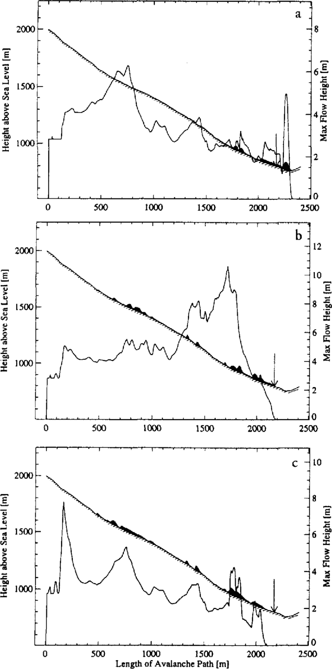
Fig. 7. Computer simulation of Mettlenruns avalanche, showing maximum flow heights. (a) Voellmy-fluid model; (b) Russian yield-stress model; (c) Norwegian NIS model. The flow heights are increased by a factor of 15. The arrow marks the observed runout position.

The Russian yield-stress model predicts the observed runout distance almost exactly. It also simulates the observed 8 m high flow heights near the measurement panel well. In fact, the Russian model is the only one to predict increased flow heights towards the end of the event, after the flow has become fully developed. These occur at the point where the avalanche has reached its maximum flow velocity, i.e. in the transition zone. They occur because the Russian model does not contain a passive pressure, which makes the flow mass more rigid than in the Voellmy-fluid and Norwegian models. The Russian model also predicts significant tail depositions. The avalanche loses much of its flow mass before stopping (in contrast to the Voellmy-fluid model). A worrisome feature of the model is that it predicted too large a flow velocity (>30ms⁻¹) at the measurement panel. Since the avalanche reached the correct runout distance, this means that the deceleration was too large. Finally, the runout distance was reached, not in a single continuous motion, but in a series of waves. This “tide-like” avalanche motion is characteristic of the Russian model, and is due to the yield stress. Smaller flow heights have higher dry-friction values, so flow stops and is overtaken by waves with larger flow heights.

The Norwegian model predicts velocities similar to those in the Russian model, as well as similar track depositions. The runout distance is underestimated, but with a more exact analysis the correct result could be obtained. In contrast to the Russian model, the Norwegian model underestimates the observed flow height. In general, we found the Norwegian model was sensitive to the flow parameters. On this particular track we found that a slight change in the dry-friction value made a big difference to the predicted runout distances and flow velocities. Figure 8a shows three simulations using the Voellmy-fluid model with the dry-friction values μ = 0.25, μ = 0.30 and μ = 0.35, and Figure 8b shows three simulations using the NIS model with the dry-friction values, b = 0.45, b = 0.50 and b = 0.55. In both models, then, the dry friction varied by only 0.1. Note the large difference in predicted flow velocity for the NIS model compared to the Voellmy-fluid model. Thus, the runout distance predicted by the NIS model can be very sensitive to the dry-friction value, if b ≈ tan ψ.

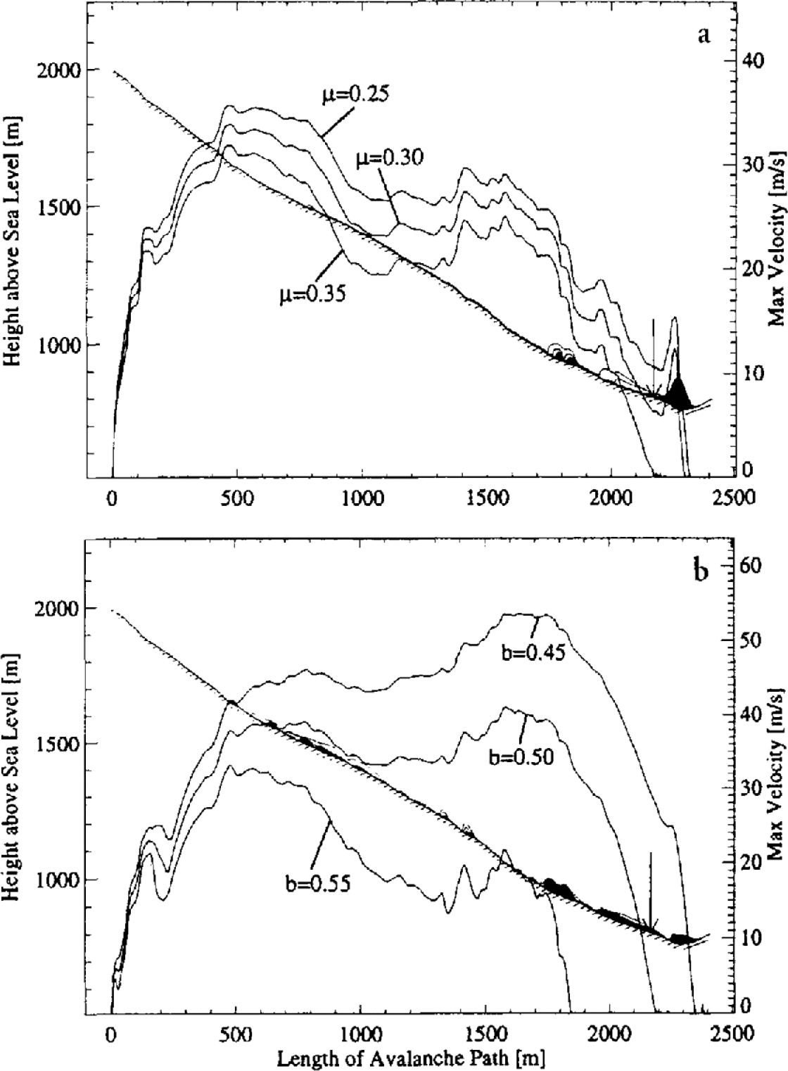
Fig. 8. Computer simulation of the Mettlenruns avalanche using (a) the Voellmy-fluid model and (b) the Norwegian NIS model. Three different dry-friction values were used for the Voellmy-fluid simulations (μ = 25, μ = 0.30 and μ = 0.35) and NIS model simulations (b = 0.45, b = 0.50 and b = 0.55). In all cases, the higher the dry friction the lower the flow velocity. Note the large difference in flow velocity predicted by the NIS model.

7. Initial Conditions and Avalanche Runout

In this section the influence of the initial conditions, specifically the initial fracture height h ₀, and fracture length l ₀, on runout distances and flow velocities is investigated. In the analysis the same test track is used as in Reference McClung and Mears.McClung and Mears (1995) and Reference Bartelt and Salm.Bartelt and Salm (in press). It consists of a 1000 m long, 25° slope and an 8° runout zone. The width of the avalanche track is everywhere w ₀ = 100 m. In all the simulations the flow parameters were held constant: μ = 0.155, = 2000 m s⁻² and λ_ρ = 2.5 over the entire length of the avalanche track. These values were chosen because they matched the runout distances of the extreme avalanche events of the Swiss Guidelines well.

In the first series of simulations the fracture height was raised from h ₀ = 0.5 m to h ₀ = 5.0 m in 0.5 m intervals. The length of the fracture zone was held constant at l ₀ = 200 m. In the second series of simulations an alternative strategy was used to increase the fracture volume: the fracture height was held constant while the length of the fracture zone was increased from l ₀ = 100 m to l ₀= 1000 m. In both cases the fracture volume was in the range 10⁴ m³ ≤ V ₀ ≤ 10⁵ m³. The results of these simulations are shown in Figure 9.

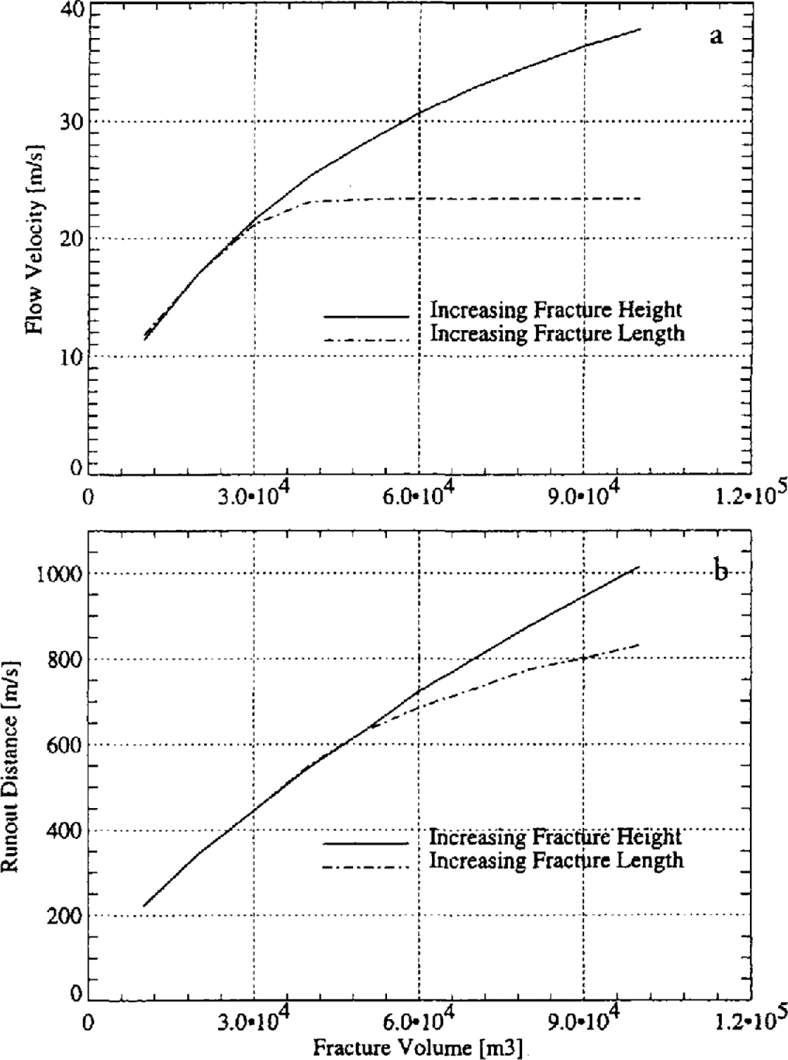
Fig. 9. (a) Flow velocity at point Pas a function of fracture volume. (b) Runout distance S as a function of fracture volume. In the first series of simulations the fracture height was increased; in the second series the fracture length was increased. For the first case the numerical model predicts that U_p α and S α h₀, which is in agreement with the VS model.

Figure 9 shows that runout distances and flow velocities are influenced greatly by the arrangement of mass in the release zone. When fracture heights are raised for a constant fracture length, runout distances S increase linearly, i.e. S α h ₀. Conversely, when fracture lengths are increased, runout distances appear to converge to a constant value. The difference between the two simulation series is even more pronounced with respect to flow velocity at point P. (Point P is located at the transition between the 25° and 8° slopes.) For the case of increasing fracture height and constant fracture length, the flow velocity at P increases according to U _p α . In the series of simulations with increasing fracture lengths, the results converge very quickly to a constant value.

An important inference from these results is that different dense-snow avalanche models cannot be compared to each other using only the initial fracture volume, or an intermediary result such as flow velocity at point P. The results clearly show that for a single fracture volume or transition-zone velocity, different runout distances are possible based on the disposition of mass in the release zone. From a practical perspective this means that exact information concerning the fracture dimensions is required in order to correctly back-calculate avalanche events. It also implies that the model avalanche “remembers” at point P how it started, i.e. how the fracture volume was dimensioned.

The calculation procedure of the Swiss Guidelines — the VS model — was used to predict avalanche runout on the same test track. The results were compared to a series of numerical simulations with three different fracture lengths (l ₀ = 200 m, l ₀ = 400 m and l ₀ = 800 m) and different fracture heights in the range 0.5 m ≤ h ₀ ≤ 3.5 m. The same flow parameters were employed in all numerical computations: μ = 0.155, = 2000 m s² and λ_ρ = 2.5. The predicted flow velocities at point P using the VS model and the numerical simulations are compared in Figure 10.

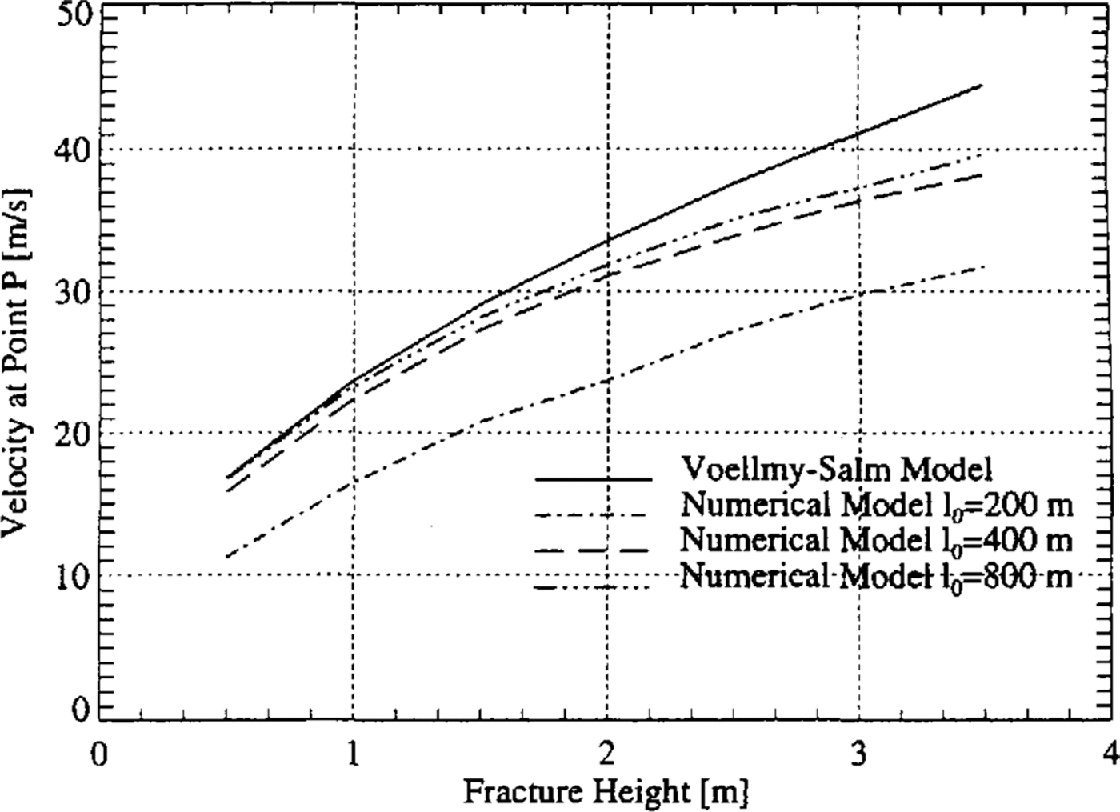
Fig. 10. Predicted terminal flow velocity for different fracture heights and lengths. Note that as the fracture length increased, the results of the numerical model converge with the VS results. Simulation parameters: μ = 0.155, ζ= 2000 m s⁻² and λ_ρ = 2.5.

Figure 10 shows that as the fracture length is increased the results from the numerical model converge with the results of the VS model. The best agreement occurs for fracture heights in the range 0.5 m ≤ h ₀ ≤ 2.0 m and long fracture lengths. The results from the first series of simulations are also apparent in this figure. The increase in flow velocity from l ₀ = 200 m to l ₀ = 400 m is greater than the increase from l ₀ = 400 m to l ₀ = 800 m. Likewise, the terminal velocity increases with increasing h ₀ at a greater rate than by increasing the fracture length. In summary, the numerical Voellmy-fluid model requires large fracture volumes in order to predict flow velocities similar to those in the VS model. This result confirms that the traditional VS model has been well calibrated for extreme avalanche events with large fracture volumes.

Despite the similarity in computed terminal velocity for large fracture volumes, the VS and the numerical Voellmy-fluid model will not predict the same flow height in the runout zone. Results from the numerical simulations for different fracture heights, h ₀, and the largest fracture length l ₀ = 800 m, are compared to the predicted VS model deposition heights in Figure 11.

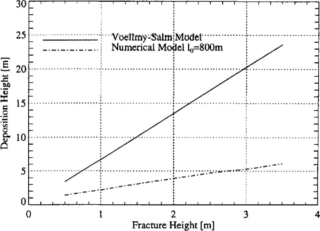
Fig. 11. Predicted deposition heights for the Swiss Guideline VS model and numerical Voellmy-fluid model. Even for large fracture volumes, the numerical model predicts smaller deposition heights.

An important inference from this result is that the numerical model requires larger values to obtain runout distances similar to those in the VS model, to compensate for the smaller flow heights in the runout zone.

The present Swiss Guideline procedures for avalanche calculation are based on the selection of a fracture height h ₀, which is related to an avalanche return period. Numerical models, as used here, require in addition to this value the fracture length, l ₀. This means that the fracture length must also be related to a return period for a particular terrain. This is a formidable task and an absolute prerequisite for the (predictive) application of numerical models in practice. To ascertain how the fracture length could be specified, it is necessary to compare the VS and numerical models further. In the next series of numerical calculations, runout distances are related directly to different fracture volumes. To compensate for the fact that the numerical model predicts significantly smaller flow heights in the runout zone, however, different values are used. The numerical computations are carried out using = 2000 m s⁻², whereas the VS calculations use = 1000 m s⁻².

Figure 12 plots runout distance against fracture heights. The runout distances of the numerical model were calculated using three different fracture lengths (l ₀ = 200 m, l ₀ = 400 m and l ₀ = 800 m). The results show that for fracture lengths l ₀ ˃ 400 m the numerical model predicts larger runout distances for equal fracture heights; for l ₀ ˂ 200 m it predicts shorter runout distances. These fracture lengths are reasonable for extreme avalanche events, suggesting again that the VS model has been well calibrated for large fracture volumes. The VS model results also increase linearly between the two curves l ₀ = 200 m and l ₀ = 400 m. Thus, a better way of interpreting these results is to state that the VS model appears to increase fracture length, from l ₀ = 200 m to l ₀ = 400 m, as the fracture height is increased from h ₀ = 0.5 m to h ₀ = 3.5 m. Moreover, the VS model assumes a specific relation between fracture height and length. For this particular problem we have found this relation to be

. (22)

From the standpoint of the numerical model the VS model does not increase fracture volume linearly, but quadratically with h ₀. This is why the VS model is so sensitive to the fracture height, as pointed out by Reference McClung and Mears.McClung and Mears (1995). It should be emphasized that Equation (22) is valid only for this particular problem and cannot be applied to other terrains. When the fracture lengths of the numerical model are chosen according to this formula, the runout distances of the Guideline and numerical models can be brought into very good agreement. This is shown in Figure 13a.

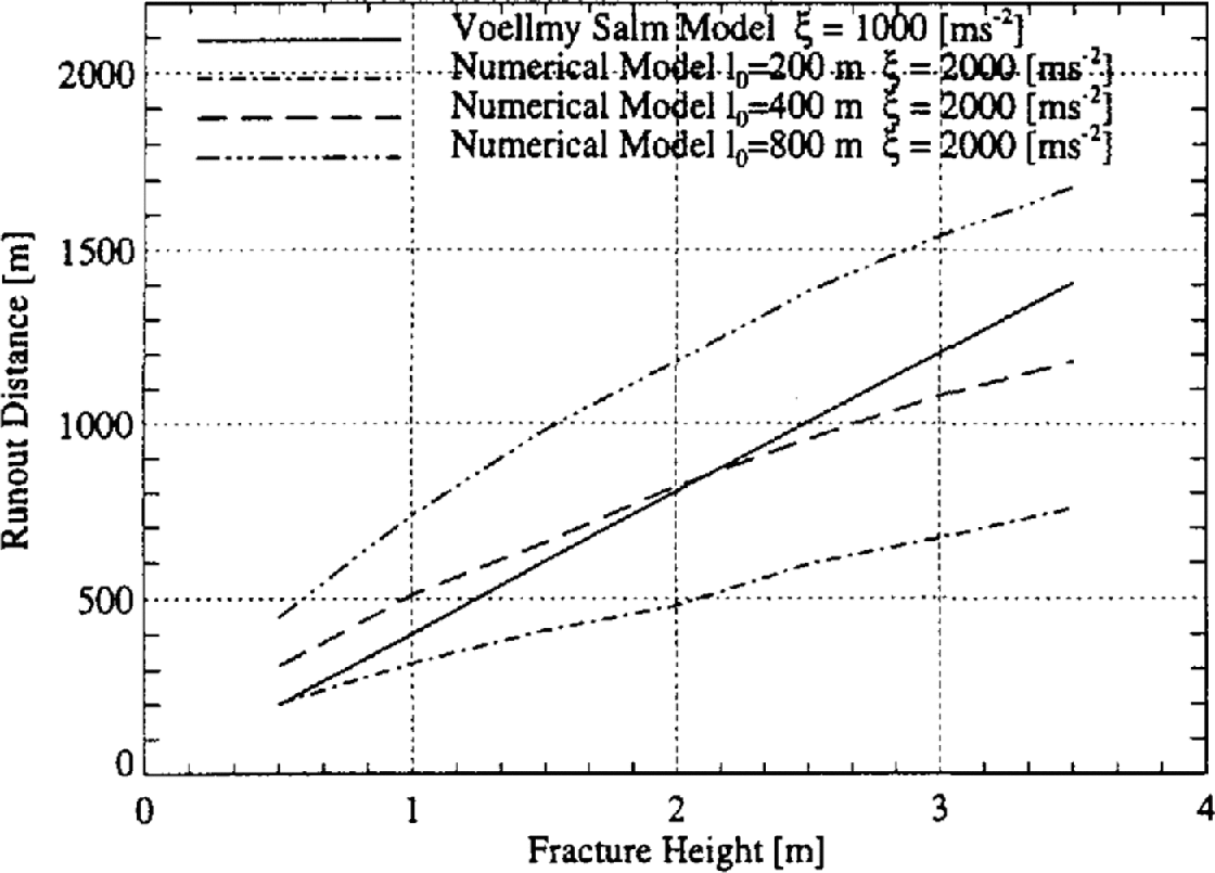
Fig. 12. Runout distance S vs fracture height h₀ for different fracture lengths.

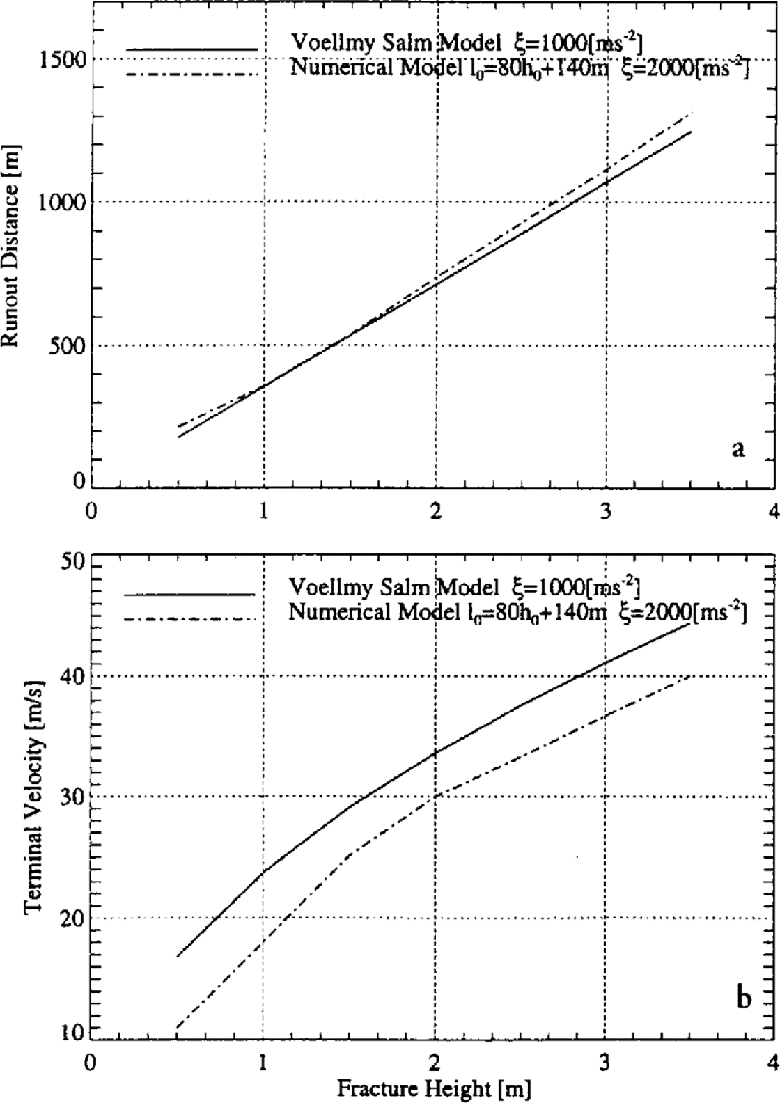
Fig. 13. (a) Runout distance S vs fracture height h₀ using Equation (22). (b) Velocity at point P U_p us fracture height h₀ using Equation (22).

It is important to recall that the VS model calculations have been carried out using = 1000 m s², whereas the numerical model used = 2000 m s⁻². As discussed above, this modification is necessary to compensate for the too large flow heights predicted by the VS model in the runout zone. Subsequently, the correspondence between the two models is not as good in velocity space. The relationship between velocity at point P and runout distance using Equation (22) is shown in Figure 13b.

8. Conclusions

In this paper a numerical dense-snow avalanche model has been presented which is now being tested for avalanche runout predictions in Switzerland. The numerical model has been used to simulate both laboratory chute experiments and actual avalanche events. The model does not require the specification of point P, determines the motion of the leading edge of the avalanche, calculates the distribution of avalanche snow in the deposition zone and predicts significantly smaller deposition heights than the traditional VS model. Thus, the numerical model resolves many of the shortcomings of the traditional VS model.

The numerical model has been constructed such that it contains two additional flowing-avalanche models, the Norwegian NIS model and the Russian yield-stress model.

The main difference between the NIS model and the Swiss Voellmy-fluid model is the assumption of plug flow. In its present formulation, the NIS model assumes that the entire flow height is fluidized, i.e. shear strain rates exist within the entire flow body. The velocity at the top flowing surface is higher than the basal sliding velocity. The shear strain rate is directly related to surface roughness. In the Voellmy-fluid model, shear strains are concentrated at the sliding base; internal flow resistance is governed only by the active/passive flow state. We believe that the Voellmy-fluid assumption of a highly cohesive flow material moving primarily in a plug-flow regime represents dense-snow avalanche behavior more accurately, especially in the runout zone.

At present, we find the NIS model difficult to apply in practical avalanche-dynamics calculations because a set of well-calibrated flow parameters does not exist. In certain terrain, such as Mettlenruns, the simulation results are very sensitive to the choice of dry friction. The model, in general, predicts higher (and in the case of Mettlenruns, unrealistic) flow velocities than the Voellmy-fluid model.

Despite these physical and practical objections, in previous work (Reference Bartelt, Salm. and HestnesBartelt and Salm, 1998) we have found that the NIS model can simulate both field experiments and the extreme avalanche case-studies of the Swiss Guidelines well. Furthermore, the mathematical formulation of the model clearly distinguishes between internal flow resistance and sliding friction because it is based on a clearly defined constitutive law and a basal slip condition. We therefore regard the NIS model as a possible precursor to more sophisticated avalanche-dynamics models which will contain both a plug-flow and a fluidized layer regime. Until such a model is developed, the Voellmy-fluid model, although an oversimplification of avalanching snow behavior, can be used for practical avalanche-dynamics calculations.

Russian researchers have modified the Voellmy-fluid model by limiting the dry friction by a yield stress. This modification produces three important effects:

1. 1. It allows both large and small avalanches to be modeled with similar and, compared to the Swiss Guidelines, higher dry-friction values.

2. 2. Because larger dry-friction values are employed, the model predicts significantly more tail depositions on steep track segments.

3. 3. Avalanche motion is not continuous, but occurs In a wave-like motion.

These are all interesting additions to the Swiss Voellmy-fluid model. As shown in the Mettlenruns case-study, the modifications certainly bring the experimentally measured and applied dry-friction values into much better agreement. They also allow the simulation of many processes, such as track deposition, which are observed in real avalanche events. Gutter’s flowing-avalanche velocity measurements near the Lukmanier pass, however, did not reveal a wave-like motion. From a practical standpoint, it is not clear whether these effects can be included in a real avalanche-dynamics calculation. In an actual case-study, the analyst must assume a “worst-case scenario”. This means, for example, assuming that the avalanche does not lose mass during its downward motion. The analyst would also have to assume that the avalanche reaches its target in one strong motion, not in successive waves of lesser intensity. In the end, the analyst must assume a small yield stress. This is similar to using a Voellmy-fluid model with a small dry-friction value. (They are not equal since the dry friction would not depend on the normal force.)

Before numerical models are introduced in practice, one avalanche-dynamics problem must be be confronted in more detail: the specification of the initial fracture conditions. In this paper, we have investigated in detail the influence of fracture height and length on predicted avalanche runout. The fracture dimensions have been found in which the unsteady numerical Voellmy-fluid model converges with the traditional VS model. We have discovered that the present Swiss Guidelines on avalanche runout implicitly define an extreme avalanche to have not only higher fracture depths but also longer fracture lengths. This procedure could be explicitly adopted by the Guidelines, but must first be analyzed. Well-formulated guideline procedures must be devised to determine initial fracture dimensions before models that track the motion of an avalanche from initiation to runout can be used in practice.

Finally, an important advantage of the Eulerian formulation adopted in the numerical solution is that a two-dimensional model, where the changing flow width of the avalanche in three-dimensional terrain is simulated, can easily be developed from the one-dimensional model presented here. This step has, in fact, already been accomplished, again using a Voellmy-fluid model with active/ passive longitudinal straining (Reference Gruber, Bartelt., Haefner. and HestnesGruber and others, 1998). However, more work comparing model results to avalanche experiments is required before results of this recent development can be introduced in the Guidelines.