


Introduction
Melting over the past century on many glaciers and ice caps has been greater than during any other period of the preceding several millennia (Reference Anderson, Miller, Briner, Lifton and VogelAnderson and others, 2008; Reference Sharp, Burgess, Cogley, Ecclestone, Labine and WolkenSharp and others, 2011a; Reference FisherFisher and others, 2012; Reference ThompsonThompson and others, 2013). The near-worldwide retreat of glacier ice has resulted in accelerating contributions of glaciers to global sea-level rise (SLR) (e.g. Reference MeierMeier and others, 2007; Reference Church and WhiteChurch and White, 2011; Gardner and others, 2013) and it is projected that glacier surface mass loss alone will contribute 0.16–0.22 ± 0.04 m to SLR during the next century (Reference Radić, Bliss, Beedlow, Hock, Miles and CogleyRadić and others, 2014). Mountain glaciers, in particular, are extremely sensitive to changes in climate (e.g. Reference MeierMeier, 1984) and some have endured rapid disintegration over the past decade (e.g. Reference Paul, Maisch, Kellenberger and HaeberliPaul and others, 2004), leading to projections that half of all small mountain glaciers (5 km2) will disappear in the next century (e.g. Reference Radić and HockRadić and Hock, 2011). With the advent of remote-sensing technologies, the ability to survey glacierized landscapes has vastly improved over the past 40 years (Pellilka and Rees, 2009). Satellite sensors such as the Advanced Spaceborne Thermal Emission and Reflection Radiometer (ASTER) and Landsat have enabled the construction of complete, precise glacier inventories in otherwise inaccessible locations (Reference Kääb, Paul, Maisch, Hoelzle and HaeberliKääb, 2005). Automated and semi-automated glacier classification techniques and the widespread availability of digital elevation models (DEMs) have increased overall mapping resolution and accuracy while decreasing classification time (e.g. Reference Kääb, Paul, Maisch, Hoelzle and HaeberliKääb and others, 2002; Reference PaulPaul and Kääb, 2005).
Initiated in 1998, the Global Land Ice Measurements from Space (GLIMS) project has as its primary goal to map and monitor all the world’s glaciers using data from satellite sensors (Reference BishopBishop and others, 2004; Reference Racoviteanu, Paul, Raup and ArmstrongRacoviteanu and others, 2009). The GLIMS program has led to comprehensive glacier inventories in many polar and alpine regions and contributes to regional glacier change assessments (e.g. Reference Knoll, Kerschner, Heller and RastnerKnoll and others, 2009; Reference PaulPaul and Andreassen, 2009; Reference Barrand and SharpBarrand and Sharp, 2010; Reference Bolch, Menounos and WheateBolch and others, 2010; Paul and Svoboda, 2010; Reference Davies and GlasserDavies and Glasser, 2012; Reference PanPan and others, 2012). As a result, glacier inventories utilizing GLIMS protocols have contributed to a near-globally complete dataset of glacier outlines (Reference ArendtArendt and others, 2013). The Torngat Mountains of northern Labrador (Fig. 1 inset),are one of the few remaining glacierized regions in the Arctic yet to be comprehensively inventoried as part of the GLIMS initiative and there is currently little baseline information available on the state of glaciers and ice masses in the region. These features occupy the southern limit of glacierization in the eastern Canadian Arctic, making them of particular interest for scientific study.
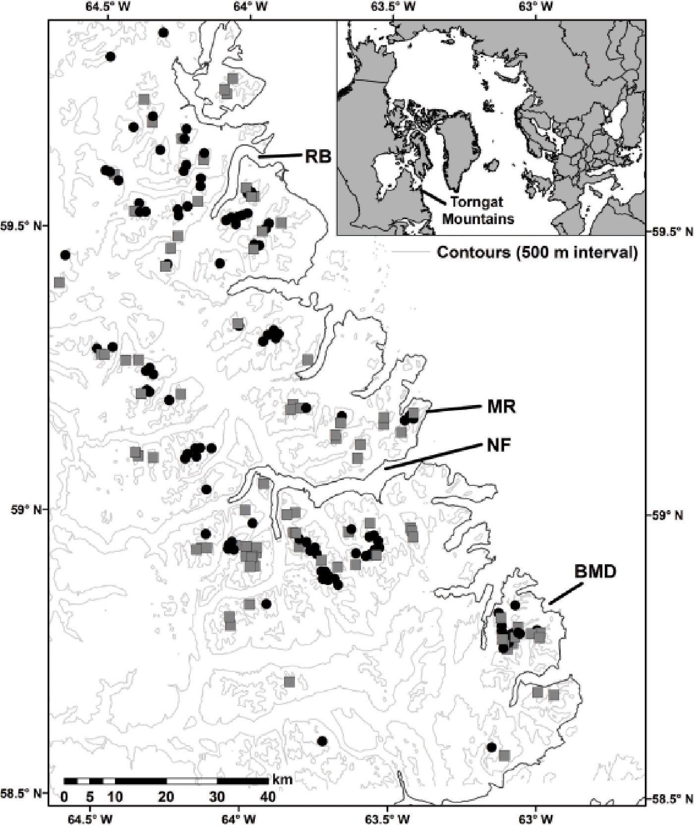
Fig. 1. Map of the Torngat Mountains and adjacent coastline. Symbols depict ice masses mapped in 2005 for this study (black circles: active ice masses; grey squares: inactive ice masses). Locations discussed in the text are abbreviated on the map as follows: Blow Me Down Mountains (BMD), Nachvak Fiord (NF), Mount Razorback (MR) and Ryan's Bay (RB). The location of the Torngat Mountains is shown relative to circum-arctic and middle northern latitudes (inset).
This paper presents the first complete inventory and classification of the ice masses of the Torngat Mountains. Adopting standard protocols established by GLIMS, the study compiles baseline data on Torngat ice masses and examines local and regional setting in detail. Trends in ice mass morphometry, geographic location and topographic setting are presented and compared with those from other northern alpine environments. The challenges encountered in mapping and classifying Torngat ice masses according to the GLIMS framework are also discussed. For the purposes of this study, we use the term ice mass to include all mapped glaciers and ice masses in the Torngat Mountains while the term glacier is used exclusively for the subset of ice masses that display signs of active flow.
Study Area
The Torngat Mountains are the southernmost mountain range in the eastern Canadian Arctic and are the only zone of Arctic Cordillera south of Baffin Island (Fig. 1). They are characterized by prominent relief in excess of 1000 m, with the highest peaks occurring ~ 20 km inland south of Nachvak Fiord (Mount Caubvick, 1652 m a.s.l.). Geologically, the Torngat Mountains are defined by the Torngat Orogen, with the regional geology being primarily of Precambrian to Archean age (Reference Wardle, Kranendonk, Mengel and ScottWardle and others, 1992). The region consists of both the Churchill and Nain provinces (Reference Wardle, Gower, Ryan, Nunn, James and KerrWardle and others, 1997). The bedrock geology is mostly orthogneiss and granite near the coast and undifferentiated gneiss farther inland (~40 km from the coast), though there are sections of sedimentary rocks in the south and several intrusions of igneous rocks in the north (Reference ClarkClark, 1991; Reference Wardle, Gower, Ryan, Nunn, James and KerrWardle and others, 1997).
The Torngat Mountains form part of the Canadian Shield and contain two main physiographic regions: the George Plateau stretching from Ungava Bay to the Quebec–Labrador drainage divide; and the fretted mountains within 40 km of the Labrador Sea coastline (Bostock, 1970). The George Plateau slopes upwards at ~ 10 m km-1 from near sea level in Ungava Bay to a maximum height of ~ 1000 m a.s.l. in the Torngat Mountains (Fig. 2a). Maximum elevations occur in the central Torngat Mountains, with decreasing elevation northwards (Fig. 2b). The fretted coastal mountains contain the greatest relief (>1000 m) with widespread cirque development. By contrast, inland cirques are less numerous and mostly form along the margins of the upland plateau. Selective linear erosion during previous glaciations of the region has resulted in the dramatic fiord and deep valley systems that predominantly run west–east through the Torngat Mountains (e.g. Reference MarquetteMarquette and others, 2004; Reference StaigerStaiger and others, 2005).
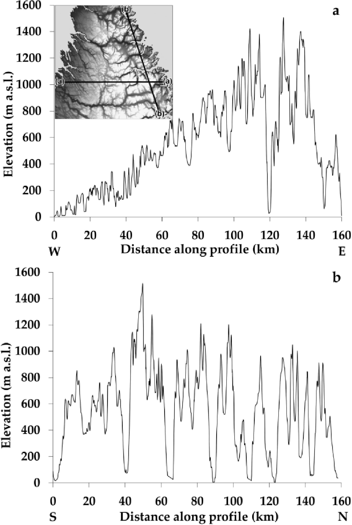
Fig. 2. Topographic profiles across the Torngat Mountains extracted from a Canadian National Topographic Database DEM. (a) West– east longitudinal transect from Ungava Bay in the west to the Labrador Sea coastline along latitude 58.8° N. (b) South–north latitudinal transect from Saglek Fiord to Eclipse River inland of the Labrador Sea coastline.
Climate
The Torngat Mountains are classified as polar tundra (ET) under the Köppen–Geiger climate classification (Reference Kottek, Grieser, Beck, Rudolf and RubelKottek and others, 2006), with the most similar bioclimatic regions located in eastern Baffin Island, West Greenland, northern Sweden and Svalbard (Reference Metzger, Sayre, Trabucco and ZomerMetzger and others, 2013). Synoptically, the Labrador Current has a pervasive influence on regional climate in the Torngat Mountains by transporting cold Arctic water southwards along the coast (Reference Banfield and JacobsBanfield and Jacobs, 1998). During the summer this leads to maritime conditions with lower temperatures and pervasive fog; in the winter, however, the formation of seasonal sea ice on the Labrador Sea leads to very cold and dry continental conditions (Reference MaxwellMaxwell, 1981). Regional wintertime precipitation (i.e. snowfall) is generated by medium- to low-intensity winter storms that are steered by the Canadian Polar Trough, which influences the positions of the Polar and Arctic fronts in northeastern Canada. Prevailing winds in the Torngat Mountains are generally greatest in the winter and lowest in the summer, with the predominant wind direction being westerly, though complex topography creates much local variability (Canadian Wind Energy Atlas; www.windatlas.ca) (e.g. Frey-Buness and others, 1995; Benoit and others, 2002).
Summary climate data for the Torngat Mountains (58.2–60.4° N, 62.2–64.3° W) are estimated using ERA-Interim reanalysis (Reference Dee, Federici and PappalardoDee and others, 2011) due to the lack of reliable weather stations in the region (e.g. Reference Way and ViauWay and Viau, in press) and because it has been shown to accurately model changes in Arctic precipitation and temperature (Reference Lindsay, Wensnahan, Schweiger and ZhangLindsay and others, 2014; Reference Cowtan and WayCowtan and Way, 2014). Over the period 1979– 2009, mean annual air temperatures were –6.2 and –8.5°C at the surface (2 m a.s.l.) and 850 mbar (~1500 m a.s.l.), respectively (Fig. 3).The 850 mbar height approximates the elevation of the highest ice masses in the Torngat Mountains. Mean summer temperatures (June–August) varied between 4.9°C at the surface and 2.7°C at 850 mbar. Total precipitation in the region averaged 0.73 m a-1 between 1979 and 2009, with most precipitation occurring in the fall (~230 mm) and summer (~210 mm).
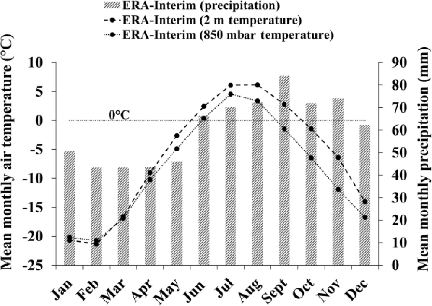
Fig. 3. Average monthly precipitation and monthly temperature for the Torngat Mountains derived from ERA-Interim reanalysis for the period 1979–2009 (Reference Dee, Federici and PappalardoDee and others, 2011). Monthly temperatures provided for both 2 and ~ 1500 m a.s.l. (850 mbar) altitude. Dotted horizontal line depicts 0°C.
Torngat ice masses
The earliest observations on ice masses in the Torngat Mountains date to the early 20th century (e.g. Reference OdellOdell, 1933), while systematic mapping by Reference Forbes, Miller, Odell, Abbe, Buness, Heimann and SausenForbes and others (1938) and Reference Henoch and StanleyHenoch and Stanley (1968) generated two preliminary inventories that identified ~ 60 ice masses north of Nachvak Fiord. Mass-balance data were collected between 1981 and 1984 on four glaciers in the Selamiut Range, south of Nachvak Fiord, by Reference RogersonRogerson (1986). Results indicated overall negative mass balance for three of the four glaciers (Reference RogersonRogerson, 1986), and the importance of snowfall accumulation in local glacier mass balance and glacier debris cover for surface melt rates (Reference Rogerson, Olson and BransonRogerson and others, 1986a). The mass-balance records support areal changes on ten glaciers between 1964 and 1979 measured by Reference StixStix (1980), of which the majority (eight) were either stagnant or retreating. Reference McCoyMcCoy (1983) and Reference Rogerson and CoyRogerson and others (1986b) both explored historical glacier variability and glacial geomorphology in several glacierized valleys south of Nachvak Fiord. Reference McCoyMcCoy (1983) dated maximum Neoglacial activity to within the past 4000 years, with abandonment of Little Ice Age (LIA) moraines in the early 15th century. In contrast, Reference Rogerson and CoyRogerson and others (1986b) attributed a much more recent age (~1000 years ago) to Neoglacial advances and placed the retreat from LIA positions to within the past 100 years.
More recently, in a pilot study of change detection on a subset of the 96 largest Torngat glaciers, Reference Brown, Allard and LemayBrown and others (2012) documented a 9% decrease in ice area between 2005 and 2008 using glacier outlines mapped from SPOT5 (Satellite Pour l’Observation de la Terre) imagery (2008) and this study (2005). The recent reduction of glacier ice in the Torngat Mountains was interpreted as a response to both higher summer air temperatures and a multi-decadal decline in winter precipitation (Reference Brown, Allard and LemayBrown and others, 2012). A full analysis of change detection over the past 60 years for all glaciers and ice masses in the Torngat Mountains, including field surveys, is currently in progress.
Methods
Data collection
Ice masses were mapped using late-summer (August 2005) 1: 40 000 colour aerial photography provided by Parks Canada. Photographs were scanned at 1 m ground resolution and orthorectified in the remote-sensing software PCI Geomatica to correct for terrain distortion due to high relief (e.g. Reference Kääb, Paul, Maisch, Hoelzle and HaeberliKääb, 2005). Orthorectification was conducted using image orientation parameters provided by the surveyor (X, Y, Z, Omega, Phi, Kappa) and manually collected tie points. This method was used instead of ground control points (GCPs) because of the lack of reliable GCPs across most of the region and because the former produced a lower root-mean-square error (RMSE) (~2.5 m) than the latter (~4.0 m). An 18 m resolution DEM derived from Canada’s National Topographic Database (NTB) (±15 m vertical accuracy) was used for orthorectification. In total, ~ 500 digital orthophotos were produced, allowing for each ice mass to be imaged in at least two orthophotos. Terrain parameters for each ice mass were measured from the NTB DEM provided by Parks Canada. SPOT5 high-resolution geometric (HRG) (5 m resolution, late summer 2008) and Landsat 7 Enhanced Thematic Mapper Plus (ETM+) (15 m resolution, late summer 1999) satellite data were used to search for ice masses not included in the initial air photo inventory.
Our preliminary ice mass database contained all possible ice masses, including active and inactive ice masses, and perennial ice patches. Differentiation between late-summer snowfields and ice masses was only possible where bare ice was visible on imagery. Given the resolution of the aerial photography (1 m), the minimum size limit for ice masses was set to 0.01 km2, similar to other recent studies (e.g. Reference PaulPaul and Andreassen, 2009; Reference Paul and SvobodaPaul and others, 2009; Reference Svoboda and PaulSvoboda and Paul, 2009; Reference Stokes, Shahgedanova, Evans and PopovninStokes and others, 2013). For ice mapping, this study used the GLIMS definition of a glacier and follows established GLIMS protocols (Reference Rau, Mauz, Vogt and RaupRau and others, 2005; Reference RaupRaup and Khalsa, 2010). Lateral meltwater streams and lakes were used to trace indistinct ice margins. Mapping of ice masses with heavy debris cover followed the assumed geometric shape of the ice mass, in addition to consideration of debris banding, flowlines and changes in surface slope (e.g. Reference Rau, Mauz, Vogt and RaupRau and others, 2005; Reference Racoviteanu, Paul, Raup and ArmstrongRacoviteanu and others, 2009). Ice masses were also obliquely viewed in three dimensions by draping satellite images and aerial photographs over the DEM in ESRI’s ArcScene to aid in the visual interpretation and classification of ice boundaries.
Mapping error assessment
Total error for mapped ice margins is difficult to quantify due to the lack of in situ margin measurements covering the same period as the aerial photography and because of inherent discrepancies in the mapping technique used by different operators (e.g. Reference PaulPaul and others, 2013). Following the recommendations of Reference PaulPaul and others (2013), two operators independently re-mapped the margins of 11 ice masses (10% of total ice area) that were selected to reflect the characteristics of the overall population (e.g. debris-covered/debris-free, large/small, shadowed/unshadowed). The RMS difference between the inventory subsets (0.007 km2) corresponds to a mapping error of ~ 2 m along ice mass margins. We use a buffer of ± 5 m on either side of our mapped ice margins to integrate cumulative errors from mapping (~2.0 m), orthorectification (~2.5 m) and planimetry, as suggested by Reference Granshaw and FountainGranshaw and Fountain (2006) and Reference Bolch, Menounos and WheateBolch and others (2010).
GLIMS classification
Ice mass classification was aided through the use of colour aerial photography, satellite imagery, limited field observations and consultation with historical aerial photography. Classification followed the protocols established by GLIMS and used the GLIMS Analysis Tutorial (Reference RaupRaup and Khalsa, 2010), GLIMS Glacier Classification Manual (Reference Rau, Mauz, Vogt and RaupRau and others, 2005) and several comprehensive publications (Reference RaupRaup and others, 2007; Reference Racoviteanu, Paul, Raup and ArmstrongRacoviteanu and others, 2009). The adapted classification scheme proposed by the GLIMS Antarctic Regional Center was used because it incorporates a parameter that quantifies the debris cover on a glacier (Reference Rau, Mauz, Vogt and RaupRau and others, 2005, Reference Rau, Kargel and Raup2006). Under this classification scheme, ice masses were first classified from ten primary glacier types, and then from nine different forms. Although not discussed in this paper, several other parameters were reported following GLIMS protocols including ice mass frontal characteristics, longitudinal profile, presumed major source of nourishment, recent activity of glacier tongue, presence of moraines and debris coverage of glacier tongue.
Active glacier ice
Ice masses with evidence of glacier flow were subdivided in the database, and their characteristics compared with those of inactive ice masses. Glacier flow was recognized through the identification of crevasses, debris banding and foliations (Fig. 4). Looped debris banding and transverse crevasses, for example, common on Torngat glaciers, are indicative of differential glacier movement (Benn and Evans, 2010). The absence of evidence of active flow for an individual ice mass does not preclude the possibility of actively flowing ice; however, without visible evidence of flow, an ice mass could not be classified as an active glacier.

Fig. 4. Aerial photograph of an actively flowing mountain glacier near Ryan's Bay (52.53° N 64.00° W) in the Torngat Mountains. The image is labeled with examples of glaciological features that categorize glacier flow.
Ice mass distribution, morphometry and topographic setting
A variety of morphometric and topographic parameters were collected to summarize the local setting of Torngat ice masses in relation to their altitudinal and spatial distributions. This computation mostly followed methods provided in Reference DeBeer and SharpDeBeer and Sharp (2009) and Paul and others (2010). Aspect was measured following the median flowline in cardinal directions (N, NE, NW, S, SE, SW, W, E). Length (km) was measured along ice mass centre lines parallel to flow direction while distance to coast was measured as the Euclidean distance (km) between ice mass centroids and the nearest Labrador Sea coastline. Area-weighted elevation (m a.s.l.; minimum, mean, maximum) and mean slope (°) were determined by collecting the zonal statistics from DEM and slope rasters of ice mass polygons. This method was also used to calculate mean area-weighted incoming solar radiation (W h m–2 ) using clear-sky insolation (direct and diffuse) calculated for the melt season midpoint (1 August) in ArcGIS 10 (Reference Fu, Rich and GardnerFu and Rich, 2002).
Debris cover (%) included only the debris cover that obscured underlying ice surfaces for each ice mass. Compactness, a measure of ice mass shape and morphometry, was collected using the formula (4π Area)/(Perimeter2) after Reference DeBeer and SharpDeBeer and Sharp (2009). Mean back-wall height was calculated from the elevation difference between a glacier basin’s ridge crest and the upper ice margin parallel to the back-wall ridge. Relative upslope area was computed as a ratio between ice mass area and total upslope area, with the latter calculated as the area between each basin’s ridge crest and upper ice margin. Upslope area was also used to derive the mean contributing area slope (°) by averaging a slope raster for mapped upslope areas.
Relationships between geographic/topographic factors and ice mass characteristics were investigated through correlation analysis and visual inspection of scatter plots. Tests for the degree of association between indices used the non-parametric Spearman rho rank correlation coefficient (r s) (e.g. Reference DeBeer and SharpDeBeer and Sharp, 2009) for interval, ordinal and highly skewed indices, and the Pearson correlation coefficient (R) for continuous data that show linear relations (Reference MannMann, 2007). Additionally, ice masses were compared based on their flow activity (active vs inactive) and physiographic region (fretted vs plateau). Indices were first tested for normality using the Shapiro–Wilk test (Reference RoystonRoyston, 1995), and then the statistical significance of differences between populations was assessed using both the Student’s t –test (Reference MannMann, 2006) and the non-parametric Kolmogorov–Smirnov test (Reference ConoverConover, 1999; Reference Marsaglia, Tsang and WangMarsaglia and others, 2003).
RESULTS
Size distribution of ice masses
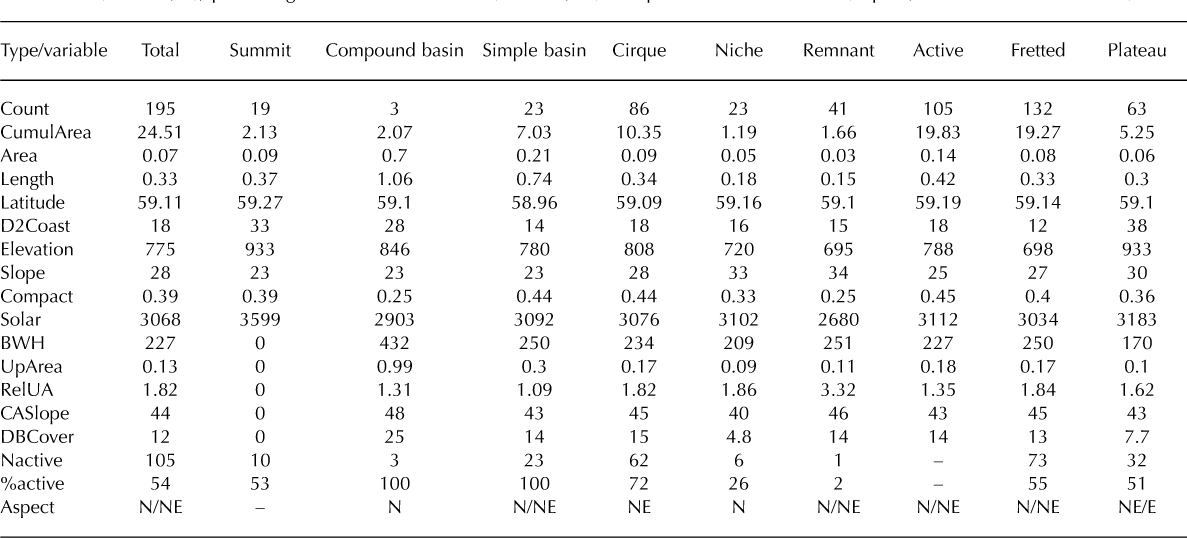
In 2005, 195 ice masses existed in the Torngat Mountains, covering a total area of 24.51 ± 1.80 km2 (Table 1).The size distribution is highly skewed to smaller ice masses, with almost a third smaller than 0.05 km2 and only eight larger than 0.5 km2 (Fig. 5). The 30 largest ice masses made up almost 50% of the total ice area, whereas the 30 smallest ice masses covered only 2.8% of the total area. The median ice mass area was 0.07 km2 (range 0.01–1.26 km2), and the median ice mass length was 0.33 km (range 0.04–2 km). In total, 49 ice masses were longer than 0.5 km, 8 longer than 1.0 km and 15 shorter than 0.1 km. Ice masses in the Torngat Mountains span slightly more than 1° of latitude (58.6–59.9° N; ~ 170 km) and occur within 50 km of the Labrador Sea (Table 1; Fig. 1). Ice masses more commonly occur in the fretted mountain region (68%; 80% of ice area) adjacent to the Labrador Sea (Table 1). For the most part, ice mass forms are evenly distributed across the region, except for summit ice masses that predominantly occur inland and farther north.
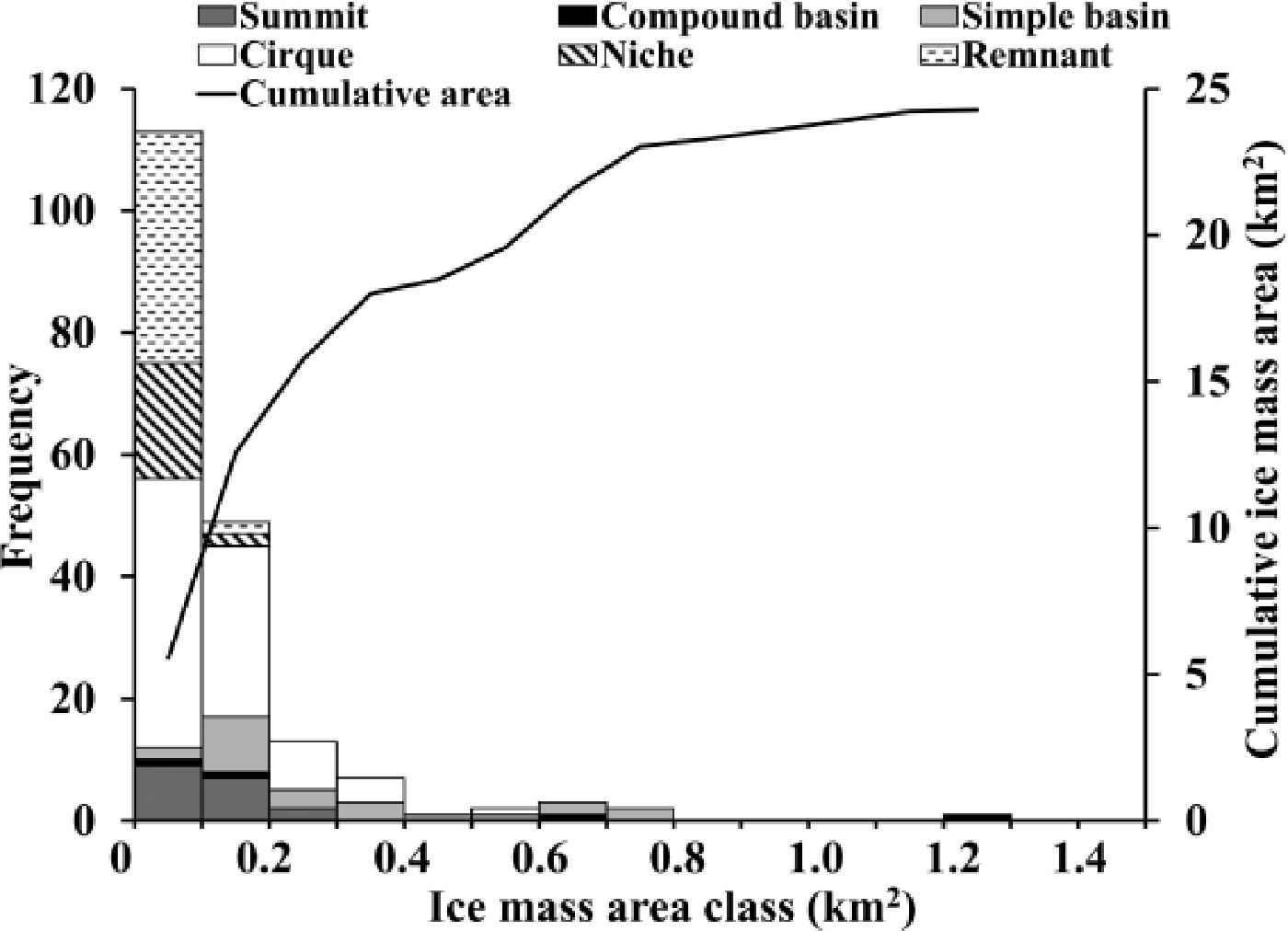
Fig. 5. Size–frequency distribution of ice masses in the Torngat Mountains. Bars are subdivided using ice mass forms classified from GLIMS protocols. Line depicts the cumulative area distribution for Torngat ice masses.
Table 1. Median values for geographic, topographic and morphometric variables subdivided by ice mass form, flow status and physiographic setting. Table includes ice mass counts (Count; n), cumulative area (CumulArea; km2), individual ice mass area (Area; km2), ice mass length (Length; km), ice mass latitude (Latitude; ° N), distance to coastline (D2Coast; km), ice mass mean elevation (Elevation; m a.s.l.), ice mass slope (Slope; °), compactness (Compact; undefined), incoming solar radiation (Solar; W h m−2), mean back-wall height (BWH; m), relative upslope area (RelUA; ratio), contributing area slope (CASlope; °), percentage debris cover (DBCover; %), count of active ice masses (Nactive; n), percentage of active ice masses (%active; %) and predominant direction (Aspect; north or north-northeast)
Classification of ice masses
Three primary ice mass types were classified in the Torngat Mountains: valley glacier (n = 1), mountain glacier (n = 96) and glacieret/snowfield (n = 94; Table 1). The most common ice mass forms were cirque (n = 86) and remnant ice (n = 41), the remainder being simple and compound basin glaciers (n = 26), niche ice masses (n = 23) and summit ice masses (n = 19). Eighty percent of the total ice area in the Torngat Mountains occurs as either cirque (42%) or simple and compound basin (38%) forms. Most Torngat ice masses (83%) have some debris cover (median percentage debris cover 13%), and roughly one-quarter are >25% debris-covered (Table 1).
Ice mass characteristics
Torngat ice masses span an elevational range between 294 (lowest ice mass snout) and 1479 m a.s.l. (highest upper ice margin) and have a median area-weighted mean elevation of 775 m a.s.l. Distance from the Labrador Sea explained about half of the variance (r 2 = 0: 51) observed in the minimum elevation of Torngat ice masses (Fig. 6), with increasingly elevated ice mass snouts farther inland (~12 m km-1 with distance from the coast). Consistent with this trend is the statistically significant difference (99% CL) between the elevations of ice mass snouts in the fretted mountains and interior plateau (Table 1). Significant differences are also observed between the mean elevations of topographically shadowed ice mass forms (e.g. niche and remnant) and less shadowed ice masses (e.g. simple basin and summit) (Table 1; Fig. 7).
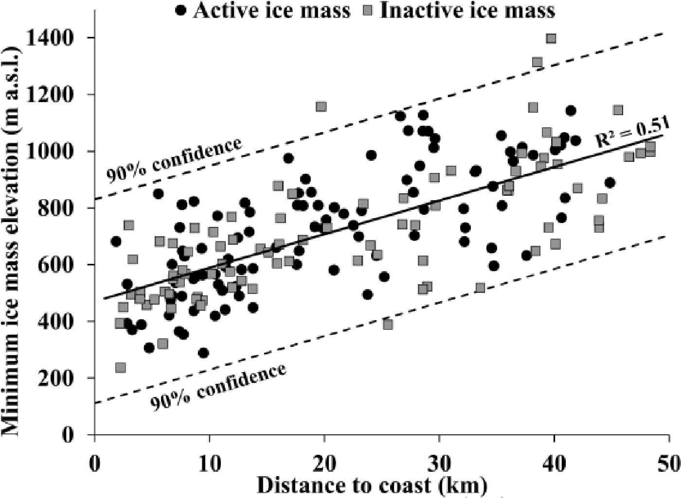
Fig. 6. Scatter plot of minimum elevation and distance from the Labrador Sea coastline for each of the Torngat ice masses. Black dots and grey squares represent active and inactive ice masses, respectively. Least-squares regression line is shown with the 90% confidence interval for lower and upper bounds.

Fig. 7. Examples of each of the six ice mass forms classified in the Torngat Mountains using GLIMS classification procedures. Images are derived from aerial photographs overlain on a DEM with black outlines depicting 2005 ice mass margins. Dialog boxes contain latitude (° N), longitude (° W), total area in 2005 (km2), mean elevation (m a.s.l.) and the distance from the Labrador Sea coastline (km) for each ice mass.
Most Torngat ice masses have a northerly aspect (63%), with the majority facing either north (23%) or northeast (28%). Ice masses rarely have a southerly aspect (11%), and even fewer are west-facing (5%). Summit, simple basin and cirque ice masses typically are more compact than niche and remnant ice masses (Table 1).
Topographic setting
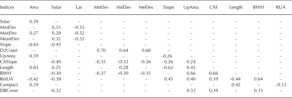
Torngat ice masses had a median back-wall height of 227 m with an interquartile range of 148–296 m (Table 1). Ice masses in the fretted mountains had higher back-walls (medians 250 vs 170 m a.s.l.) and total upslope areas (medians 0.17 vs 0.10 km2) compared to those in the interior plateau, reflecting the relatively greater relief of the coastal mountains. Most ice mass forms in the region had a relative upslope area between 1.09 and 1.86, with the exception of remnant ice masses that had higher values (median 3.32; Table 1) and summit ice masses, which by definition had no relative upslope area (Table 1). Summit ice masses had the greatest incoming solar radiation due to their relatively exposed surfaces, whereas remnant ice masses had the smallest values (Fig. 8). The results of the Spearman correlation analysis show ice mass area is negatively correlated with both mean slope and relative upslope area (Table 2). Neither result is surprising given that the smallest Torngat ice masses are typically found adhering to steep mountainsides or large cirque back-walls and the largest ice masses flow into flatter basins and valleys. Likewise, ice mass length is negatively correlated with mean slope for the same reason. Upslope area is shown to be strongly positively correlated with total ice mass area while negative correlations are found between incoming solar radiation and ice mass slope (Table 2). Statistical associations between solar radiation and three topographic parameters (contributing area slope, back-wall height, relative upslope area) suggest that ice masses receiving less solar radiation have large, steep back-walls. Incoming solar radiation is also positively correlated with ice mass elevation, implying that more exposed surfaces were found higher in the mountains while the lowest ice masses are more topographically protected (Table 2). A relation with elevation is also reflected in the classification of ice form (Fig. 8).
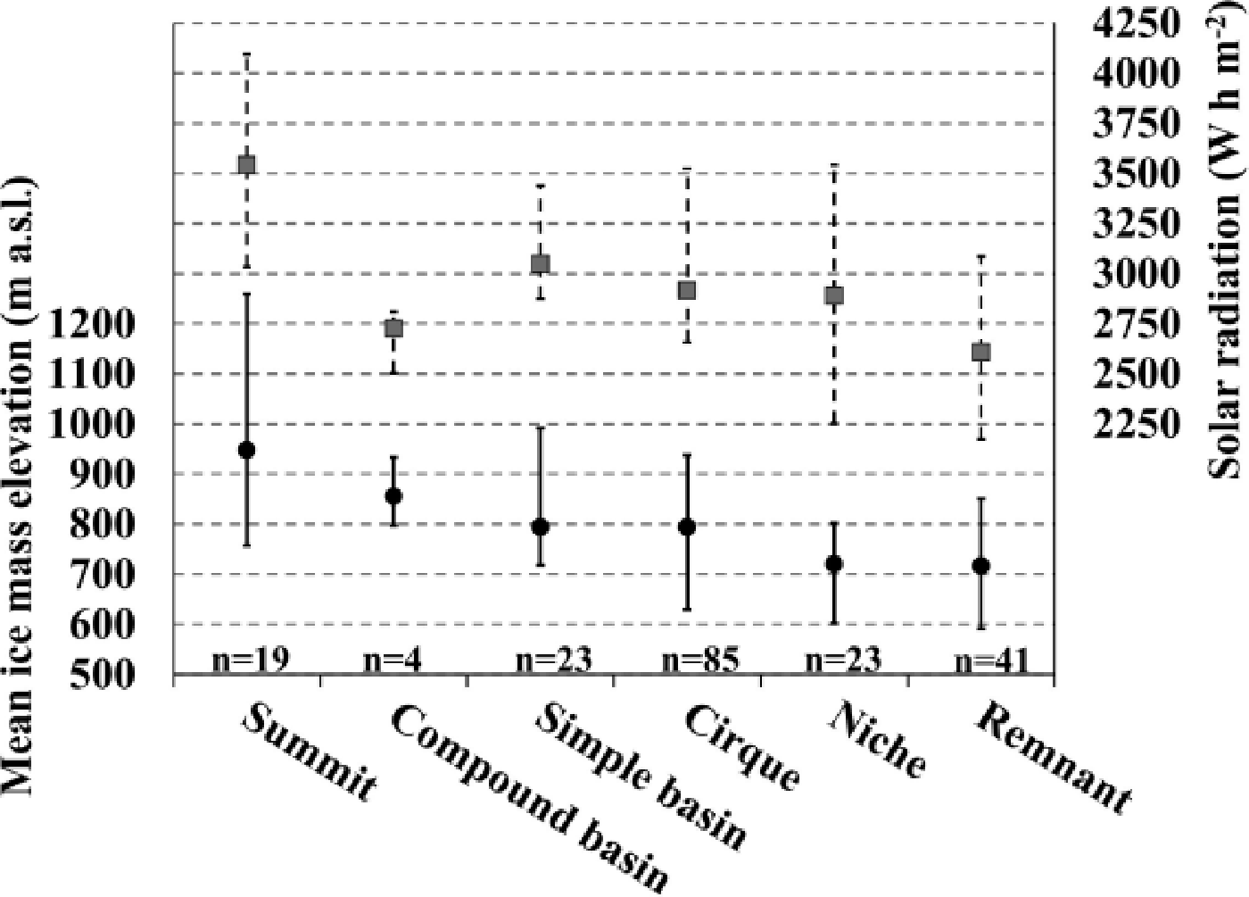
Fig. 8. Relation between ice mass form, median ice mass elevation (circles) and median incoming solar radiation (squares). Vertical lines show the interquartile range.
Table 2. Spearman rho rank correlation matrix between geographic, topographic and morphometric parameters for ice masses in the Torngat glacier inventory. Table presents correlations (r s values) for individual ice mass area (Area; km2), incoming solar radiation (Solar; W h m–2 ), ice mass latitude (Lat; ° N), minimum elevation (MinElev–MnElev; m a.s.l.), maximum elevation (MaxElev–MxElev; m a.s.l.), mean elevation (MeanElev–MeElev; m a.s.l.), ice mass slope (Slope; °), distance to coastline (D2Coast; km), total upslope area (UpArea; km2), contributing area slope (CASlope–CAS; °), ice mass length (Length; km), mean back-wall height (BWH; m), relative upslope area (RelUA– RUA; ratio), compactness (Compact; undefined) and debris cover (DBCover; %). Only statistically significant correlations (>95% CL (confidence level)) are shown
Active glaciers
In this study, 54% of ice masses showed evidence of actively flowing ice, the majority as either cirques (n = 62) or simple and compound basin forms (n = 26). Actively flowing glaciers made up ~ 20 km2 or 81% of the total ice area, and 70% of them were in the fretted coastal mountains. A similar proportion of active glaciers faced north or northeast compared to the total glacier population. Statistically significant differences between active and inactive ice masses were apparent for many variables including compactness (99% CL), debris cover (99% CL), elevation (99% CL), latitude (93% CL), length (99% CL), relative upslope area (99% CL), size (99% CL), slope (99% CL) and solar radiation (92% CL). Relative to inactive ice masses, median values show that active glaciers were typically larger, longer, more compact, slightly more northerly, higher and more debris-covered (Table 1). On average, active glaciers also had lower slopes, smaller relative upslope areas and correspondingly higher incoming solar radiation. A few variables (e.g. back-wall height and contributing area slope) showed no statistically significant differences between active and inactive ice masses.
Discussion
Torngat ice masses in local context
Our study reveals several distinct patterns in the general characteristics and geographic distribution of ice masses in the Torngat Mountains. First, most Torngat ice masses exist in topographically protected basins with the largest ice masses (simple and compound basin) almost exclusively originating in cirques with large back-walls (Fig. 8). Second, active ice masses occur at higher elevations and farther north, where melt seasons are presumably shorter and less intense (Reference DeBeer and SharpDeBeer and Sharp, 2009). Third, active ice masses are also more heavily debris-covered than inactive ice masses, further reducing melt rates (Reference Rogerson and CoyRogerson and others, 1986b). By contrast, inactive ice masses are more reliant on snow avalanching as indicated by large relative upslope areas and reduced melt rates due to topographic shadowing. Fourth, the ice-mass forms characterized by the most topographic shadowing (cirque, niche and remnant) are more numerous and receive less incoming radiation, thereby demonstrating the importance of local topography for ice preservation (Table 1). The steep upslope contributing areas on most Torngat ice masses are also important for avalanching snow onto ice surfaces, with most Torngat ice masses having upslope areas that are larger than the ice masses themselves (Reference Rogerson, Olson and BransonRogerson and others, 1986a). By contrast, summit ice masses, which lack protection from local topography and have no upslope area, receive more solar radiation and have higher elevation values, making their presence indicative of the true regional snowline in the interior (Fig. 8) (Reference Wolken, Sharp and EnglandWolken and others, 2008). The more frequent occurrence of Torngat ice masses in the fretted coast relative to the inland plateau seems to be related to regional physiography. In particular, the fretted landscape of the coastal Torngat Mountains is more dissected than the inland plateau, increasing the frequency of cirque and niche topographic settings near the coastline. The inland Torngat Mountains, though consisting of high overall elevations, are dominated by extensive plateau landscapes that provide minimal topographic protection from solar radiation and fewer niches for snow accumulation. The plateau is therefore less likely to sustain small mountain glaciers but more likely to contain larger plateau ice masses when a drop in the regional glaciation level occurs (Reference Rea, Whalley, Gordon, Dougall and OwenRea and others, 1998). This is reflected in the inventory data showing that coastal ice masses are typically larger, longer and more active than those in the interior plateau.
Ice masses in the fretted coast also have substantially lower ice elevations, with distance to the Labrador Sea coastline being the strongest predictor of all ice mass elevation parameters. The influence of maritime meteorological conditions on near-coast ice masses may explain some of this association. For example, summer fog has been shown to protect glaciers from intense summer melt by reflecting incoming solar radiation and by providing additional moisture close to ice masses (e.g. Reference Mernild, Kane, Hansen, Jakobsen, Hasholt and KnudsenMernild and others, 2008; Reference Jiskoot, Juhlin, Pierre and CitterioJiskoot and others, 2012). The pattern of dense fog and low-level cloud during the summertime in the coastal Torngat Mountains (Reference MaxwellMaxwell, 1981) supports this hypothesis. In the complex topography of the coastal Torngat Mountains, it is difficult to assess the importance of prevailing winds on snow redistribution and corresponding ice mass location. Inland along the plateau, however, ice masses predominantly face east to northeast, enhancing lee-side accumulation of snow on ice surfaces from westerly winds.
Ice mass characteristics, particularly ice mass elevation, were also found to be related to several topographic factors (e.g. CASlope, BWH, RelUA). These results suggest that ice masses with lower elevations are more reliant on mass input from avalanching potentially causing more ice flux through their equilibrium-line altitudes. The low compactness values found for niche and remnant ice masses reflect irregular-shaped ice masses fed through avalanching (Reference DeBeer and SharpDeBeer and Sharp, 2009). Given that local topography is an important factor for Torngat ice masses, it might be expected that regional geology is associated with several topographic variables (e.g. back-wall height, contributing area slope, debris cover and relative upslope area). However, examining the spatial distribution of these variables shows consistent results across the various rock types in the Torngat Mountains (e.g. Reference Wardle, Gower, Ryan, Nunn, James and KerrWardle and others, 1997). To further evaluate the importance of regional geology, we examined the distribution of mean ice mass elevation for each rock type after the influences of distance to coast and latitude had been removed with multiple regression (adjR2 = 0.49). Iterative t –tests showed that the residuals from the regression model had little spatial structure and are statistically indistinguishable across the major rock types, suggesting that regional geology is largely unrelated to ice mass distribution and elevation.
Torngat ice masses in regional perspective
The ice masses of the Torngat Mountains are on average the smallest ice masses inventoried in the Canadian Arctic and contain far less ice than other glacier populations (Reference SharpSharp and others, 2011b). Relative to their latitude they exist considerably lower in the mountains than many other mountain glaciers, particularly those in the Canadian Rockies, Swiss Alps and Scandinavia (Reference Paul, Maisch, Kellenberger and HaeberliPaul and others, 2004; Reference PaulPaul and Andreassen, 2009; Reference Andreassen and WinsvoldAndreassen and Winsvold, 2012; Reference Tennant, Menounos, Wheate and ClagueTennant and others, 2012). However, the most maritime glaciers in Iceland, coastal Norway and the coastal Rocky Mountains exist at similar elevations (Reference Nesje, Bakke, Dahl and MatthewsNesje and others, 2008; Reference Huss and FarinottiHuss and Farinotti, 2012). Glacier inventories completed on small glaciers in southern Baffin Island (64–68° N) and the Ural Mountains (64–68° N) have similar median elevations to those in the Torngat Mountains (e.g. Reference PaulPaul and Kääb, 2005; Reference PaulPaul and Svoboda, 2009; Reference Svoboda and PaulSvoboda and Paul, 2009), with the latter glaciers also being similar in size, morphometry and topographic setting (Reference Kononov, Ananicheva and WillisKononov and others, 2005; Reference Shahgedanova, Nosenko, Bushueva and IvanovShahgedanova and others, 2012).
Many authors have observed that local topographic setting has a strong influence on small glaciers in alpine environments (Reference KuhnKuhn, 1995; Reference Hoffman, Fountain and AchuffHoffman and others, 2007; Reference DeBeer and SharpDeBeer and Sharp, 2009) and that some small topographically protected glaciers have exhibited less recent change than nearby glaciers (e.g. Reference DeBeer and SharpDeBeer and Sharp, 2009; Reference Basagic, Fountain, Benn and BenoitBasagic and Fountain, 2011; Reference Li, Li, Wang and GaoLi and others, 2011; Reference Stokes, Shahgedanova, Evans and PopovninStokes and others, 2013). Federici and Pappalardo (2010) and Reference Shahgedanova, Nosenko, Bushueva and IvanovShahgedanova and others (2012) also noted that the recession of some small glaciers slowed once they receded into the most protected portions of their shadowed cirques where they receive less direct radiation. Likewise, in the Torngat Mountains most ice masses historically extended beyond their protective basins, but since have retreated up-valley into their cirques where large back-walls protect ice surfaces from incoming solar radiation (e.g. Reference DeBeer and SharpDeBeer and Sharp, 2009). The importance of high back-walls for debris transport onto Torngat ice surfaces is another relevant consideration (e.g. Reference Stokes, Shahgedanova, Evans and PopovninStokes and others, 2013) given that there are direct observations of decreased melting on debris-covered Torngat glaciers (Reference RogersonRogerson and others, 1986a). Although topographic setting influences the distribution of ice masses in the Torngat Mountains, the presence of summit ice masses at lower elevations than similar features much farther north in western Scandinavia suggests that other factors (e.g. maritime conditions) are also relevant (Reference ManleyManley, 1955; Reference Gellatly, Gordon, Whalley and HansomGellatly and others, 1988; Reference ReaRea and Evans, 2007).
Maritime conditions and coastal proximity have been shown to influence (reduce) glacier elevations in many regions (e.g. Reference Nesje, Bakke, Dahl and MatthewsNesje and others, 2008; Reference Huss and FarinottiHuss and Farinotti, 2012; Reference Jiskoot, Juhlin, Pierre and CitterioJiskoot and others, 2012). For example, the most coastal glacier ranges in southwestern and northern Norway contain the glaciers with the lowest elevations while the mountain glaciers further inland are typically restricted to the uppermost mountains (Reference Gellatly, Gordon, Whalley and HansomGellatly and others, 1988; Reference Andreassen and WinsvoldAndreassen and Winsvold, 2012). Maritime influences can also be seen when examining long-term glacier changes in southwest Norway where coastal glaciers notably advanced during the 1990s in response to increased winter snowfall while continental glaciers showed little change (Reference Chinn, Winkler, Salinger and HaakensenChinn and others, 2005). Likewise, in the Canadian Cordillera, coastal glaciers were found to be less sensitive to ablation-season temperature changes than their interior counterparts, possibly due to maritime conditions (Reference Schiefer and MenounosSchiefer and Menounos, 2010). In many of these maritime environments the survival of mountain glaciers at low elevations is due to heavy winter precipitation (e.g. Reference Nesje, Bakke, Dahl and MatthewsNesje and others, 2008). However, in the Torngat Mountains the combined effects of local topographic setting and coastal meteorological conditions explain ice mass formation at lower elevations than other mid-latitude glaciers, similar to Ural Mountains glaciers which have local conditions that favor snow accumulation in cirques (Reference Kononov, Ananicheva and WillisKononov and others, 2005; Reference Solomina, Ivanov and BradwellSolomina and others, 2010).
Regional glacierization level
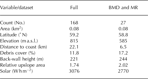
Visual examination of the relation between latitude and ice mass elevation reveals a group of low-elevation outlier ice masses impacting the least-squares fit. These ice masses are exclusively found in the coastal ranges of the Blow Me Down Mountains (BMD) and on the coastal side of Mount Razor-back (MR). Further inspection of these ice masses reveals that they exist in topographically unique settings with unusually high, steep back-walls relative to other Torngat ice masses (Table 3). They are also characteristically more heavily debris-covered, possibly due to their larger upslope contributing areas. In addition to these topographic factors, the BMD and MR ice masses exist in close proximity to the Labrador Sea (all within 10 km of the coastline), presumably reflecting the importance of local meteorological conditions. Given that these ice masses exist in a unique topographic and geographic setting, they are unlikely to be representative of the conditions experienced for most of the Torngat glaciers. By excluding these two regions, a much stronger relationship is found between ice mass elevation and latitude (r 2 = 0.47), with the slope of the regression line interpreted as the mean elevation of topographically advantaged mountain glaciers (Fig. 9). Using only ice masses classified as active this relationship is even stronger (r 2 = 0.57). Examination of ice masses with the least topographic influence (summit ice masses) shows that the regression line presented in Figure 9 is a good approximation for the minimum regional glacierization level in the Torngat Mountains.
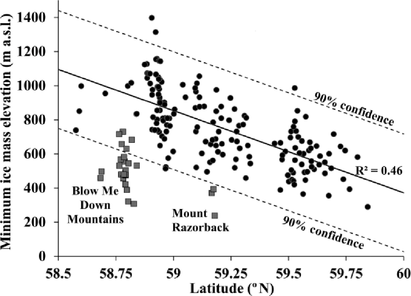
Fig. 9. Scatter plot of latitude and minimum elevation for ice masses (dots; n = 168) in the Torngat Mountains. Ice masses from the Blow Me Down Mountains and Mount Razorback are represented by grey squares (n = 27). A least-squares regression line (solid) is shown with 90% confidence intervals (dashed) for glaciers (black dots) other than those in the Blow Me Down Mountains and Mount Razorback.
Table 3. Comparison between the full Torngat ice mass inventory (excluding subset) and the ice masses of the Blow Me Down Mountains (BMD) and Mount Razorback (MR) which are investigated separately
Challenges of classification and inventorying
Most ice masses in the Torngat Mountains are small (0.1 km2), making them difficult to map on medium-resolution satellite imagery such as Landsat and ASTER. Using high-resolution imagery can increase the accuracy for mapping small ice masses; however, the cost of acquiring aerial photography or satellite imagery at high spatial resolution can be prohibitive, particularly for monitoring purposes. Pronounced topographic shadowing in the high-relief Torngat Mountains also made the process of delineating and classifying ice mass margins difficult and time-consuming (e.g. Reference Stokes, Shahgedanova, Evans and PopovninStokes and others, 2013). In some cases, shadowing may have hindered the identification of bare glacier ice and evidence of glacier flow (e.g. flowlines and crevasses). Shadowing deep in cirques may also have affected the differentiation between perennial snow and ice. Widespread debris cover on many Torngat ice masses, particularly when concentrated at lower ice elevations, may have resulted in some underestimation of ice mass size. Furthermore, medial moraines, debris ridges and thick ice-cored debris fields in the foregrounds of many Torngat ice masses complicated the delineation of the boundaries between active and inactive debris-covered ice (Reference Racoviteanu, Paul, Raup and ArmstrongRacoviteanu and others, 2010; Reference PaulPaul and others, 2013). Additionally, snowpatches on late-summer aerial photographs introduced challenges for mapping precise ice margins and potentially obscured evidence of ice flow that might otherwise have been visible during summers with limited snow cover (Reference Racoviteanu, Paul, Raup and ArmstrongRacoviteanu and others, 2009; Reference Stokes, Shahgedanova, Evans and PopovninStokes and others, 2013).
Conclusion
In this study, we have conducted the first complete inventory of ice masses in the Torngat Mountains of northern Labrador. In total, there are 195 Torngat ice masses, with the majority being actively flowing small mountain glaciers. All Torngat ice masses are located within 50 km of the coastline, where a combination of regional physiography and local meteorological conditions favor ice preservation. The topographic setting of ice masses is characterized by high back-walls, heavy debris cover and topographic shadowing. Torngat ice masses have mean elevations below other low-Arctic glaciers and occur farther south than expected based on latitude alone. We propose that unique topographical and meteorological conditions explain much of this discrepancy. By examining classification and topographic setting parameters, the data suggest that low-altitude ice masses are able to survive because of protection from solar radiation given by high back-walls and sometimes heavy debris cover. Distance to the Labrador coastline is found to be the best predictor of ice mass elevation, suggesting that local meteorological conditions may play a role in preserving ice masses in near-coastal environments. By excluding ice masses from two near-coastal sites that have unique topographic and meteorological settings (Blow Me Down Mountains and Mount Razorback), a regional glacierization level can be estimated.
Acknowledgements
We acknowledge the Torngat Mountains base camp and research station (kANGIDLUASUk), Parks Canada and Arctic Net for logistical support in the Torngat Mountains. A special thanks to our bear monitor Andreas Tuglivina and to field assistants Jodie Chadbourn, Philippe Leblanc, Svieda Mah and Alexandre Melanson. Digital elevation and remote-sensing data were provided by Parks Canada. Funding and in-kind support from ArcticNet, the Nunatsiavut Government, Memorial University of Newfoundland, the Natural Science and Engineering Research Council of Canada, the Northern Scientific Training Program and the W. Garfield Weston Foundation made this project possible. The paper benefited from discussions with or comments by Angus Simpson, Darroch Whitaker, Bob Rogerson, David Evans, Joel Finnis, Philippe Leblanc and two anonymous reviewers.


